Self-Improving Voronoi Construction for a Hidden Mixture of Product Distributions^††thanks: Research of Cheng and Wong are supported by Research Grants Council, Hong Kong, China (project no. 16200317).

Self-improving algorithms, proposed by Ailon et al. [2], is a framework for studying algorithmic complexity beyond the worst case. There is a training phase that allows some auxiliary structures about the input distribution to be constructed. In the operation phase, these auxiliary structures help to achieve an expected running time, called the limiting complexity, that may surpass the worst-case optimal time complexity.

Self-improving algorithms have been designed for product distributions [2, 10]. Let $n$ be the input size. A product distribution $\mathscr{D}=(D_{1},\ldots,D_{n})$ consists of $n$ distributions $D_{i}$ such that the $i$th input item is drawn independently from $D_{i}$. It is possible that $D_{i}=D_{j}$ for some $i\not=j$, but the draws of the $i$th and $j$th input items are independent. No further information about $\mathscr{D}$ is given. Sorting, Delaunay triangulation, 2D maxima, and 2D convex hull have been studied for product distributions. For all four problems, the training phase uses $O(n^{\varepsilon})$ input instances, and the space complexity is $O(n^{1+\varepsilon})$. The limiting complexities of sorting and Delaunay triangulation are $O\bigl{(}\frac{1}{\varepsilon}n+\frac{1}{\varepsilon}H_{\text{out}}\bigr{)}$ for any $\varepsilon\in(0,1)$, where $H_{\text{out}}$ is the entropy of the output distribution [2]. The limiting complexities for 2D maxima and 2D convex hull are $O(\mathrm{OptM}+n)$ and $O(\mathrm{OptC}+n\log\log n)$ respectively, where OptM and OptC are the expected depths of the optimal linear decision trees for the two problems [10].

Extensions that allow dependence among input items have been developed. One extension is that there is a hidden partition of $[n]$ into groups. The input items with indices in the $k$th group follow some hidden functions of a common parameter $u_{k}$. The parameters $u_{1},u_{2},\cdots$ follow a product distribution. The partition of $[n]$ is not given though. If the hidden functions are known to be linear, sorting can be solved in a limiting complexity of $O\bigl{(}\frac{1}{\varepsilon}n+\frac{1}{\varepsilon}H_{\text{out}}\bigr{)}$ after a training phase that takes $O(n^{2}\log^{3}n)$ time [8]. If it is only known that each hidden function has $O(1)$ extrema and the graphs of two functions intersect in $O(1)$ places (without knowing any of the functions, or any of these extrema and intersections), sorting can be solved in a limiting complexity of $O(n+H_{\text{out}})$ after an $\tilde{O}(n^{3})$-time training phase [7]. For the Delaunay triangulation problem, if it is known that the hidden functions are bivariate polynomials of $O(1)$ degree (without knowing the polynomials), a limiting complexity of $O(n\alpha(n)+H_{\text{out}})$ can be achieved after a polynomial-time training phase [7].

Another extension is that the input instance $I$ is drawn from a hidden mixture of at most $m$ product distributions. That is, there are at most $m$ product distributions $\mathscr{D}_{1},\mathscr{D}_{2},\ldots$ such that $\Pr[I\sim\mathscr{D}_{a}]=\lambda_{a}$ for some fixed positive value $\lambda_{a}$. The upper bound $m$ is given, but no information about the $\lambda_{a}$’s and the $\mathscr{D}_{a}$’s is provided. Sorting can be solved in a limiting complexity of $O\bigl{(}\frac{1}{\varepsilon}n\log m+\frac{1}{\varepsilon}H_{\text{out}}\bigr{)}$ after a training phase that takes $O(mn\log^{2}(mn)+m^{\varepsilon}n^{1+\varepsilon}\log(mn))$ time [8].

In this paper, we present a self-improving algorithm for constructing Voronoi diagrams under a convex distance function $d_{Q}$ in $\mathbb{R}^{2}$, assuming that the input distribution is a hidden mixture of at most $m$ product distributions. The convex distance function $d_{Q}$ is induced by a given convex polygon $Q$ of $O(1)$ size. The upper bound $m$ is given, and we assume that $m=o(\sqrt{n})$. We also assume that for each product distribution $\mathscr{D}_{a}$ in the mixture, $\lambda_{a}=\Omega(1/n)$. Let $\varepsilon\in(0,1)$ be a parameter fixed beforehand. The training phase uses $O(mn\log(mn))$ input instances and takes $O\bigl{(}mn\log^{O(1)}(mn)+m^{\varepsilon}n^{1+\varepsilon}\log(mn)\bigr{)}$ time. In the operation phase, given an input instance $I$, we can construct its Voronoi diagram $\mathrm{Vor}_{Q}(I)$ under $d_{Q}$ in a limiting complexity of $O\big{(}\frac{1}{\varepsilon}n\log m+\frac{1}{\varepsilon}n2^{O(\log^{*}n)}+\frac{1}{\varepsilon}H\bigr{)}$, where $H$ denotes the entropy of the distribution of the Voronoi diagram output. Note that $\Omega(H)$ is a lower bound of the expected running time of any comparison-based algorithm. Our algorithm also works for the Euclidean case, and the limiting complexity improves to $O\big{(}\frac{1}{\varepsilon}n\log m+\frac{1}{\varepsilon}H\bigr{)}$.

For simplicity, we will assume throughout the rest of this paper that the hidden mixture has exactly $m$ product distributions. We give an overview of our method in the following.

We follow the strategy in [2] for computing a Euclidean Delaunay triangulation. The idea is to form a set $S$ of sample points and build $\mathrm{Del}(S)$ and some auxiliary structures in the training phase so that any future input instance $I$ can be merged quickly into $\mathrm{Del}(S)$ to form $\mathrm{Del}(S\cup I)$, and then $\mathrm{Del}(I)$ can be split off in $O(n)$ expected time. Merging $I$ into $\mathrm{Del}(S)$ requires locating the input points in $\mathrm{Del}(S)$. The location distribution is gathered in the training phase so that distribution-sensitive point location can be used to avoid the logarithmic query time as much as possible. Modifying $\mathrm{Del}(S)$ efficiently into $\mathrm{Del}(S\cup I)$ requires that only $O(1)$ points in $I$ fall into the same neighborhood in $\mathrm{Del}(S)$ in expectation.

In our case, since there are $m$ product distributions, we will need a larger set $S$ of $mn$ sample points in order to ensure that only $O(1)$ points in $I$ fall into the same neighborhood in $\mathrm{Vor}_{Q}(S)$ in expectation. But then merging $I$ into $\mathrm{Vor}_{Q}(S)$ in the operation phase would be too slow because scanning $\mathrm{Vor}_{Q}(S)$ already requires $\Theta(mn)$ time. We need to extract a subset $R\subseteq S$ such that $R$ has $O(n)$ size and $R$ contains all points in $S$ whose Voronoi cells conflict with the input points.

Still, we cannot afford to construct $\mathrm{Vor}_{Q}(R)$ in $O(n\log n)$ time. In the training phase, we form a metric $d$ related to $d_{Q}$ and construct a net-tree $T_{S}$ for $S$ under $d$ [16]. In the operation phase, after finding the appropriate $R\subseteq S$, we use nearest common ancestor queries [22] to compress $T_{S}$ in $O(n\log\log m)$ time to a subtree $T_{R}$ for $R$ that has $O(n)$ size. Next, we use $T_{R}$ to construct a well-separated pair decomposition of $R$ under $d$ in $O(n)$ time [16], use the decomposition to compute the nearest neighbor graph of $R$ under $d$ in $O(n)$ time, and then construct $\mathrm{Vor}_{Q}(R)$ from the nearest neighbor graph in $O(n)$ expected time. The merging of $I$ into $\mathrm{Vor}_{Q}(R)$ to form $\mathrm{Vor}_{Q}(R\cup I)$, and the splitting of $\mathrm{Vor}_{Q}(R\cup I)$ into $\mathrm{Vor}_{Q}(I)$ and $\mathrm{Vor}_{Q}(R)$ are obtained by transferring their analogous results in the Euclidean case [2, 6].

We have left out the expected time to locate the input points in $\mathrm{Vor}_{Q}(S)$. It is bounded by $O(1/\varepsilon)$ times the sum of the entropies of the point location outcomes. We show that $\mathrm{Vor}_{Q}(I)$ allows us to locate the input points in $\mathrm{Vor}_{Q}(S)$ in $O(n\log m+n2^{O(\log^{*}n)})$ time. Then, a result in [2] implies that the sum of the entropies of the point location outcomes is $O(n\log m+n2^{O(\log^{*}n)}+H)$. The expected running time is thus $O(\frac{1}{\varepsilon}n\log m+\frac{1}{\varepsilon}n2^{O(\log^{*}n)}+\frac{1}{\varepsilon}H)$, which dominates the limiting complexity. In the Euclidean case, $\mathrm{Vor}(I)$ allows us to locate the input points in $O(n\log m)$ time, so the limiting complexity improves to $O(\frac{1}{\varepsilon}n\log m+\frac{1}{\varepsilon}H)$.

Let $Q$ be a convex polygon that has $O(1)$ complexity and contains the origin in its interior. Let $\partial$ and $\mathrm{int}(\cdot)$ be the boundary and interior operators, respectively. So $Q$’s boundary is $\partial Q$ and its interior is $\mathrm{int}(Q)$. Let $d_{Q}$ be the distance function induced by $Q$: $\forall\,x,y\in\mathbb{R}^{2}$, $d_{Q}(x,y)=\min\{\lambda\in[0,\infty):y\in\lambda Q+x\}$. As $Q$ may not be centrally symmetric (i.e., $x\in Q\iff-x\in Q$), $d_{Q}$ may not be a metric.

The bisector of two points $p$ and $q$ is $\{x\in\mathbb{R}^{2}:d_{Q}(p,x)=d_{Q}(q,x)\}$, which is an open polygonal curve of $O(1)$ size. The Voronoi diagram of a set $\Sigma$ of $n$ points, $\mathrm{Vor}_{Q}(\Sigma)$, is a partition of $\mathbb{R}^{2}$ into interior-disjoint cells $V_{p}(\Sigma)=\{x\in\mathbb{R}^{2}:\,\forall q\in\Sigma,\,d_{Q}(p,x)\leq d_{Q}(q,x)\}$ for all $p\in\Sigma$. There are algorithms for constructing $\mathrm{Vor}_{Q}(\Sigma)$ in $O(n\log n)$ time [9, 19].

$V_{p}(\Sigma)$ is simply connected and star-shaped with respect to $p$ [9]. We use $N_{p}(\Sigma)$ to denote the set of Voronoi neighbors of $p$ in $\mathrm{Vor}_{Q}(\Sigma)$. The Voronoi edges of $\mathrm{Vor}_{Q}(\Sigma)$ form a planar graph of $O(|\Sigma|)$ size. Each Voronoi edge is a polygonal line, and we call its internal vertices Voronoi edge bends. We use $V_{\Sigma}$ to denote the set of Voronoi edge bends and Voronoi vertices in $\mathrm{Vor}_{Q}(\Sigma)$. For the infinite Voronoi edges, their endpoints at infinity are included in $V_{\Sigma}$.

Define $Q^{*}=\{-x:x\in Q\}$. For any points $x,y\in\mathbb{R}^{2}$, $d_{Q^{*}}(x,y)=d_{Q}(y,x)$. At any point $x$ on a Voronoi edge of $\mathrm{Vor}_{Q}(\Sigma)$ defined by $p,q\in\Sigma$, there exists $\lambda\in(0,\infty)$ such that $d_{Q^{*}}(x,p)=d_{Q}(p,x)=d_{Q}(q,x)=d_{Q^{*}}(x,q)=\lambda$ and $d_{Q^{*}}(x,s)=d_{Q}(s,x)\geq\lambda$ for all $s\in\Sigma$. Hence, $\{p,q\}\subset\partial(\lambda Q^{*}+x)$ and $\mathrm{int}(\lambda Q^{*}+x)\cap\Sigma=\emptyset$, i.e., an “empty circle property”.

Take a point $x$. Consider the largest homothetic²²2A homothetic copy of a shape is a scaled and translated copy of it. copy $Q^{*}_{x}$ of $Q^{*}$ centered at $x$ such that $\mathrm{int}(Q^{*}_{x})\cap\Sigma=\emptyset$. If we insert a new point $q$ to $\Sigma$, we say that $q$ conflicts with $x$ if $q\in Q^{*}_{x}$. We say that $q$ conflicts with a cell $V_{p}(\Sigma)$ if $q$ conflicts with some point in $V_{p}(\Sigma)$. Clearly, $V_{p}(\Sigma)$ must be updated by the insertion of $q$. We use $V_{\Sigma}|_{q}$ to denote the subset of $V_{\Sigma}$ that conflict with $q$. The Voronoi edge bends and Voronoi vertices in $V_{\Sigma}|_{q}$ will be destroyed by the insertion of $q$.

We make three general position assumptions. First, no two sides of $Q$ are parallel. Second, for every pair of input points, their support line is not parallel to any side of $Q$. Third, no four input points lie on the boundary of any homothetic copy of $Q^{*}$, which implies that every Voronoi vertex has degree three.

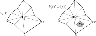
It is much more convenient if all Voronoi cells of the input points are bounded. We assume that all possible input points appear in some fixed bounding square $\cal B$ centered at the origin. We place $O(1)$ dummy points outside $\cal B$ so that all Voronoi cells of the input points are bounded, and their portions inside $\cal B$ remain the same as before. Refer to Figure 1. Take $\lambda Q^{*}$ for some large enough $\lambda\in\mathbb{R}$ such that for every point $x\in{\cal B}$, $\lambda Q^{*}+x$ contains $\cal B$. Refer to the left image in Figure 1. We slide a copy of $\lambda Q^{*}$ around $\cal B$ to generate the outer convex polygon. The dashed polygon demonstrates the sliding of $\lambda Q^{*}$ around $\cal B$. This outer polygon contains a translational copy of every edge of $\cal B$ and two translational copies of every edge of $\lambda Q^{*}$. We add the vertices of this outer polygon as dummy points. Any homothetic copy of $Q^{*}$ that intersects $\cal B$ cannot be expanded indefinitely without containing some of these dummy points. So all Voronoi cells of input points are bounded. For each point $x\in{\cal B}$, since the dummy points lie outside $\lambda Q^{*}+x$ and ${\cal B}\subseteq\lambda Q^{*}+x$ (i.e., $\lambda Q^{*}+x$ is not empty of the input points), the portion of the Voronoi diagram inside $\cal B$ is unaffected by the dummy points.

Construct a point location structure $L_{S}$ for the triangulated $\mathrm{Vor}_{Q}(S)$ with $O(\log(mn))$ query time [13]. Take another $m^{\varepsilon}n^{\varepsilon}$ input instances and use $L_{S}$ to locate the points in these input instances in the triangulated $\mathrm{Vor}_{Q}(S)$. For every $i\in[n]$ and every triangle $t$, we compute $\tilde{\pi}_{i,t}$ to be the ratio of the frequency of $t$ hit by $p_{i}$ to $m^{\varepsilon}n^{\varepsilon}$, which is an estimate of $\Pr[p_{i}\in t]$. For each $i\in[n]$, form a subdivision ${\cal S}_{i}$ that consists of triangles with positive $\tilde{\pi}_{i,t}$’s, triangulate the exterior of ${\cal S}_{i}$, and give these new triangles a zero estimated probability. Set the weight of each triangle in ${\cal S}_{i}$ to be the maximum of $(mn)^{-\varepsilon}$ and its estimated probability. Construct a distribution-sensitive point location structure $L_{i}$ for ${\cal S}_{i}$ based on the triangle weights [1, 17]. Note that $L_{i}$ has $O(m^{\varepsilon}n^{\varepsilon})$ size, and locating a point in a triangle $t\in{\cal S}_{i}$ takes $O\bigl{(}\log\frac{W_{i}}{w_{t}}\bigr{)}$ time, where $w_{t}$ is the weight of $t$ and $W_{i}$ is the total weight in ${\cal S}_{i}$.

For any input instance $(p_{1},\ldots,p_{n})$ in the operation phase, we will query $L_{i}$ to locate $p_{i}$ in the triangulated $\mathrm{Vor}_{Q}(S)$, which may fail if $p_{i}$ falls into a triangle with zero estimated probability. If the search fails, we query $L_{S}$ to locate $p_{i}$.

Let $d$ be the metric induced by the centrally symmetric convex polygon $\hat{Q}$, which is a doubling metric—there is a constant $\lambda>0$ such that for any point $x\in\mathbb{R}^{2}$ and any positive number $r$, the ball with respect to $d$ centered at $x$ with radius $r$ can be covered by $\lambda$ balls with respect to $d$ of radius $r/2$.

Given a set of points $P$, a net-tree for $P$ with respect to $d$ [16] is an analog of the well-separated pair decomposition for Euclidean spaces [4]. It is a rooted tree whose leaves are the points in $P$. For each node $v$, let $\mathit{parent}(v)$ denote its parent, and let $P_{v}$ denote the subset of $P$ at the leaves that descend from $v$. Every tree node $v$ is given a representative point $p_{v}$ and an integer level $\ell_{v}$. Let $\tau\geq 11$ be a fixed constant. Let $B(x,h)$ denote the ball $\{y\in\mathbb{R}^{2}:d(x,y)\leq h\}$. By the results in [16] (Definition 2.1 and the remark that follows Proposition 2.2), the following properties are satisfied by a net-tree:

1. (a)

   $p_{v}\in P_{v}$.

2. (b)

   For every non-root node $v$, $\ell_{v}<\ell_{\mathit{parent}(v)}$, and if $v$ is a leaf, then $\ell_{v}=-\infty$.

3. (c)

   Every internal node has at least two and at most a constant number of children.

4. (d)

   For every node $v$, $B\bigl{(}p_{v},\frac{2\tau}{\tau-1}\cdot\tau^{\ell_{v}}\bigr{)}$ contains $P_{v}$.

5. (e)

   For every non-root node $v$, $B\bigl{(}p_{v},\frac{\tau-5}{2\tau-2}\cdot\tau^{\ell_{\mathit{parent}(v)}-1}\bigr{)}\cap P\subset P_{v}$.

6. (f)

   For every internal node $v$, there is a child $w$ of $v$ such that $p_{w}=p_{v}$.

We assign nodes in each cluster a unique cluster index in the range $[1,O(n)]$. We also assign each node of a cluster three indices from the range $[1,O(m)]$ according to its rank in the preorder, inorder, and postorder traversals of that cluster. The preorder and postorder indices allow us to tell in $O(1)$ time whether two nodes are an ancestor-descendant pair.

We keep an initially empty van Emde Boas tree $\mathit{EB}_{c}$ [23] with each cluster $c$. The universe for $\mathit{EB}_{c}$ is the set of leaves in the cluster $c$, and the inorder of these leaves in $c$ is the total order for $\mathit{EB}_{c}$. We also build a nearest common ancestor query data structure for each cluster [22]. The nearest common ancestor query of any two nodes can be reported in $O(\log\log m)$ time.

Extract the subset $B\subset S$ of points whose Voronoi cell boundaries contain some region boundary vertices in the $m^{2}$-division. So $|B|=O(m\cdot n/m)=O(n)$. Compute $\mathrm{Vor}_{Q}(B)$ and triangulate it as in triangulating $\mathrm{Vor}_{Q}(S)$. By our choice of $B$, the region boundaries in the $m^{2}$-division of $\mathrm{Vor}_{Q}(S)$ form a subgraph of $\mathrm{Vor}_{Q}(B)$. Label in $O(n)$ time the Voronoi edge bends and Voronoi vertices in $\mathrm{Vor}_{Q}(B)$ whether they exist in $\mathrm{Vor}_{Q}(S)$.

We construct point location data structures for every region $\Pi$ in the $m^{2}$-division as follows. For every boundary vertex $w$ of $\Pi$, let $Q^{*}_{w}$ be the largest homothetic copy of $Q^{*}$ centered at $w$ such that $\mathrm{int}(Q^{*}_{w})\cap B=\emptyset$. These $Q^{*}_{w}$’s form an arrangement of $O(m^{2})$ complexity, and we construct a point location data structure that allows a point to be located in this arrangement in $O(\log m)$ time. We also construct a point location data structure for the portion of the triangulated $\mathrm{Vor}_{Q}(S)$ inside $\Pi$. Since the region has $O(m^{2})$ complexity, this point location data structure can return in $O(\log m)$ time the triangle in the triangulated $\mathrm{Vor}_{Q}(S)$ that contains a point inside $\Pi$.

Lemma 3.1(a) leads to Lemma 3.2 below, which implies that for any $v\in V_{S}$, if we feed the input points that conflict with $v$ to a procedure that runs in quadratic time in the worst case, the expected running time of this procedure over all points in $V_{S}$ is $O(n)$. The proof of Lemma 3.2 is just an algebraic manipulation of the probabilities, and it is given in Appendix B.

We state two technical results. Their proofs are in Appendix B. Figure 3(a) and (b) illustrate these two lemmas.

Given an instance $I=(p_{1},\cdots,p_{n})$, we construct $\mathrm{Vor}_{Q}(I)$ using the pseudocode below.

Operation Phase

1. 1.

   For each $i\in[n]$, query $L_{i}$ to find the triangle $t_{i}$ in the triangulated $\mathrm{Vor}_{Q}(S)$ that contains $p_{i}$, and if the search fails, query $L_{S}$ to find $t_{i}$.

2. 2.

   For each $i\in[n]$, search $\mathrm{Vor}_{Q}(S)$ from $t_{i}$ to find $V_{S}|_{p_{i}}$, i.e., the subset of $V_{S}$ that conflict with $p_{i}$. This also gives the subset of $S$ whose Voronoi cells conflict with the input points. Let $R$ be the union of this subset of $S$ and the set of representative points of all cluster roots in $T_{S}$.

3. 3.

   Compute the compression $T_{R}$ of $T_{S}$ to $R$.

4. 4.

   Construct the nearest neighbor graph 1-$\mathrm{NN}_{R}$ under the metric $d$ from $T_{R}$.

5. 5.

   Compute $\mathrm{Vor}_{Q}(R)$ from 1-$\mathrm{NN}_{R}$.

6. 6.

   Modify $\mathrm{Vor}_{Q}(R)$ to produce $\mathrm{Vor}_{Q}(R\cup I)$.

7. 7.

   Split $\mathrm{Vor}_{Q}(R\cup I)$ to produce $\mathrm{Vor}_{Q}(I)$ and $\mathrm{Vor}_{Q}(R)$. Return $\mathrm{Vor}_{Q}(I)$.

We analyze step 1 in Section 4.1, steps 2 and 3 in Section 4.2, steps 4 and 5 in Section 4.3, and steps 6 and 7 in Section 4.4. Step 1 is the most time-consuming; all other steps run in $O(n)$ expected time or $O(n\log\log m)$ expected time.

References

- [1] S. Arya, T. Malamatos, D.M. Mount, and K.C. Wong. Optimal expected-case planar point location. SIAM Journal on Computing, 37 (2007), 584–610.
- [2] N. Ailon, B. Chazelle, K. Clarkson, D. Liu, W. Mulzer, and C. Seshadhri. Self-improving algorithms. SIAM Journal on Computing, 40 (2011), 350–375.
- [3] K. Buchin and W. Mulzer. Delaunay triangulations in time and more. Journal of the ACM, 58 (2011), 6:1–6:27.
- [4] P.B. Callahan and S.R. Kosaraju. A decomposition of multidimensional point sets with applications to -nearest-neighbors and -body potential fields. Journal of the ACM, 42 (1995), 67–90.
- [5] T.M. Chan. A simpler linear-time algorithm for intersecting two convex polyhedra in three dimensions. Discrete & Computational Geometry, 56 (2016), 860–865.
- [6] B. Chazelle, O. Devillers, F. Hurtado, M. Mora, V. Sacristan, and M. Teillaud. Splitting a delaunay triangulation in linear time. Algorithmica, 34 (2002), 39–46.
- [7] S.-W. Cheng, M.-K. Chiu, K. Jin, and M.T. Wong. A generalization of self-improving algorithms. Proceedings of the International Symposium on Computational Geometry, 2020, 29:1–29:13. Full version: arXiv:2003.08329v2.
- [8] S.-W. Cheng, K. Jin, and L. Yan. Extensions of self-improving sorters. Algorithmica, 82 (2020), 88–106.
- [9] L. Paul Chew and R.L. Scot Drysdale. Voronoi diagrams based on convex distance functions. Proceedings of the 1st Annual Symposium on Computational Geometry, 1985, 235–244.
- [10] K.L. Clarkson, W. Mulzer, and C. Seshadhri. Self-improving algorithms for coordinatewise maxima and convex hulls. SIAM Journal on Computing, 43(2):617–653, 2014.
- [11] K.L. Clarkson and P.W. Shor. Applications of random sampling in computational geometry, II. Discrete and Computational Geometry, 4 (1989), 387–421.
- [12] T.M. Cover and J.A. Thomas. Elements of Information Theory. Wiley-Interscience, New York, 2nd edition, 2006.
- [13] H. Edelsbrunner, L.J. Guibas, and J. Stolfi. Optimal point location in a monotone subdivision. SIAM Journal on Computing, 15 (1986), 317–340.
- [14] G.N. Frederickson. Fast algorithms for shortest paths in planar graphs, with applications. SIAM Journal on Computing, 16 (1987), 1004–1022.
- [15] M.L. Fredman. How good is the information theory bound in sorting? Theoretical Computer Science, 1(4):355 – 361, 1976.
- [16] S. Har-Peled and M. Mendel. Fast construction of nets in low-dimensional metrics and their applications. SIAM Journal on Computing, 35 (2006), 1148–1184.
- [17] J. Iacono. Expected asymptotically optimal planar point location. Computational Geometry: Theory and Applications, 29 (2004), 19–22.
- [18] K. Junginer and E. Papadopoulou. Deletion in abstract Voronoi diagram in expected linear time. Proceedings of the 34th International Symposium on Computational Geometry, 2018, 50:1–50:14.
- [19] R. Klein, K. Mehlhorn, and S. Meiser. Randomized incremental construction of abstract Voronoi diagrams. Computational Geometry: Theory and Applications, 3 (1993), 157–184.
- [20] G.L. Miller, S.-H. Teng, W. Thurston, and S.A. Vavasis. Separators for sphere-packings and nearest neighbor graphs. Journal of the ACM, 44 (1997), 1–29.
- [21] E. Pyrga and S. Ray. New existence proofs for -nets. Proceedings of the 24th Annual Symposium on Computational Geometry, 2008, 199–207.
- [22] A.K. Tsakalides and J. van Leeuwen. An optimal pointer machine algorithm for finding nearest common ancestors. Technical Report RUU-CS-88-17, Department of Computer Science, University of Utrecht, 1988.
- [23] P. van Emde Boas, R. Kaas, and E. Zijlstra. Design and implementation of an efficient priority queue. Mathematical Systems Theory, 10 (1977), 99–127.
- [24] R.W. Yeung. A First Course in Information Theory, Kluwer Academic/Plenum Publishers, 2002.
Appendix A Proof of Lemma 3.1
We restate Lemma 3.1 and then give its proof.
Statement of Lemma 3.1: Let , , be the distributions in the hidden mixture. The training phase computes the following structures in time.
-
(a)
A set of points and . It holds with probability at least that for any and any , , where if conflicts with and otherwise.
(b)
Point location structures and for each that allow us to locate in the triangulated in expected time, where is the random variable that represents the point location outcome, and is the entropy of the distribution of .
(c)
A net-tree for , the clusters in , the initially empty van Emde Boas trees for the clusters, and the nearest common ancestor data structures for the clusters.
(d)
An -division of , the subset of points whose Voronoi cell boundaries contain some region boundary vertices in the -division, , and the point location data structures for the regions in the -division.
Proof. Let be the set of points from which the -net was extracted. The set consists of this -net and the dummy points. Let be a triple of distinct indices. Let be the homothetic copy of that circumscribes , and if it exists; otherwise, we ignore . Assume that is not ignored. We analyze the number of points in any input instance that fall inside .
Fix any product distribution in the hidden mixture. Let . How large is ? Since , the expected size of is . Then, Chernoff bound implies that with probability at least .
For every , define if ; otherwise, . Let . The variables ’s are independent from each other, so the Chernoff bound is applicable to . It says that for any , .
If , then . Setting gives . There are fewer than triples of distinct indices. By the union bound, it holds with probability at least that for any triple of distinct indices, if , then .
Consider any Voronoi vertex and its defining triple . If , then because is a -net of . But is empty as is a Voronoi vertex, which implies that . If we restrict our attention to instances in that contribute to , the count does not get bigger. That is, . By the contrapositive of the result that we obtained earlier on the relation between and , we conclude that . Moreover, this upper bound on hold simultaneously for all defining triples of the Voronoi vertices in with probability at least .
Since the input distribution is oblivious of the training and operation phases, we can use the instances in to derive the following inequality: . The additive term of stems from the fact that the indices in are excluded from in the definition of , but they are allowed in . Rearranging terms gives
As discussed before, the above result holds for with probability at least . Applying the union bound over all , we get a success probability of at least .
Consider (b). If falls into a triangle with weight , the distribution-sensitive point location data structure [1, 17] ensures that the query time of is , where . Since is defined to be and the complexity of is , we have . Let be the true probability of hitting a triangle in the triangulated . Using the Chernoff bound, one can prove as in [2, Lemma 3.4] that, with probability at least , for every and every , if , then . As , if , the query time is . If , we may query as well, so the query time is . Therefore, the expected query time of is bounded by .
Appendix B Missing details in Section 3
We restate the results below and give their proofs.
Statement of Lemma 3.2: For every , let be the subset of input points that conflict with . It holds with probability at least that .
Proof. For every and every , define if and otherwise.
Lemma 3.1(a) is invoked in the third step. The last step is due to the fact that and . Under the condition that , and are independent. Therefore, . As a result,
In the last step, we use Lemma 3.1(a) and the relations that and .
Statement of Lemma 3.3: Consider for some point set . For any point , let be the largest homothetic copy of centered at such that . Let and be two adjacent Voronoi edge bends or Voronoi vertices in . For any point , . The same property holds if and are Voronoi vertices connected by a Voronoi edge, and lies on that Voronoi edge.
Proof. We assume that is not equal to or as there is nothing to prove otherwise. Let and be two of the defining points of and . So and lie on the Voronoi edge defined by and . Place an imaginary point in such that does not lie on the same edge of as or . Place an imaginary point similarly in . Figure 5(a) shows an example.