∎
Bunkyo-cho 3, Hirosaki, Aomori 036-8561, Japan
W. Kurebayashi 33institutetext: Department of Mechanical Science and Engineering, Graduate School of Science and Technology, Hirosaki University
Bunkyo-cho 3, Hirosaki, Aomori 036-8561, Japan
M. Hisakado 44institutetext: Nomura Holdings, Inc., Otemachi 2-2-2, Chiyoda-ku, Tokyo 100-8130, Japan
Self-exciting negative binomial distribution process and critical properties of intensity distribution
Abstract
We study the continuous time limit of a self-exciting negative binomial process and discuss the critical properties of its intensity distribution. In this limit, the process transforms into a marked Hawkes process. The probability mass function of the marks has a parameter , and the process reduces to a ”pure” Hawkes process in the limit . We investigate the Lagrange–Charpit equations for the master equations of the marked Hawkes process in the Laplace representation close to its critical point and extend the previous findings on the power-law scaling of the probability density function (PDF) of intensities in the intermediate asymptotic regime to the case where the memory kernel is the superposition of an arbitrary finite number of exponentials. We develop an efficient sampling method for the marked Hawkes process based on the time-rescaling theorem and verify the power-law exponents.
1 Introduction
Recently, high-frequency financial data have become available, and many studies have been devoted to calibrating models of market micro-structure(Bacry et al. 2015). Initially, many studies adopted discrete time models that captured trade dynamics at regular time intervals or through a sequence of discrete time events, such as trades. Subsequently, the framework of the continuous time model—the point process— has been gradually applied to model financial data at the transaction level (Hasbrouck 1991, Engle and Russell 1998, Bowsher 2007, Hawkes 1971a, b, Hawkes and Oakes 1974, Hawkes 2018, Filimonov and Sornette 2012, 2015, Wheatley et al. 2019).
A point or counting process is characterized by its ”intensity” function, which represents the conditional probability of an event occurring in the immediate future. The Hawkes process, introduced by A. G. Hawkes (Hawkes 1971a, b, Hawkes and Oakes 1974), is a type of point process originally developed to model the occurrence of seismic events. Owing to its simplicity and flexibility, this model is being increasingly used in high-frequency finance (Bacry et al. 2015, Kirchner 2017, Blanc et al. 2017, Errais et al. 2010). It can easily capture the interactions between different types of events, incorporate the influence of intensive factors through marks, and accommodate non-stationarities.
The non-stationarity of the Hawkes process arise from the reproduction of an event induced by the interaction terms described by the kernel function that estimate the effect of the past events based on the elapsed time from them. The intensity of the process is determined by summing the effects of all past events through the kernel function. Additionally, by introducing a real number ”mark” that represents the strength of event effects, both the marks and the kernel values can be considered in the intensity estimation. If the average number of events triggered by one event, known as the branching ratio, exceeds one, the system becomes non-stationary. If the branching ratio approaches one from below, the system becomes critical, leading to power-law scaling in the PDF of the intensities in the intermediate asymptotic region. In the sub-critical case, the distribution decays exponentially beyond the characteristic intensity, which diverges as the branching ratio approaches one (Kanazawa and Sornette 2020b, a).
The discrete time self-exciting negative binomial distribution (DT-SE-NBD) was proposed for the modeling of time-series data related to defaults (Hisakado and Mori 2020). This model incorporates a parameter that captures the correlation of events within the same term, and the process converges to a discrete-time self-exciting Poisson process in the limit . In the context of time-series default data, defaults are typically recorded on a yearly or quarterly basis, and defaults within the same period exhibit high correlation. Consequently, the probability distribution of the number of defaults displays overdispersion, where the variance is significantly larger than the mean value. To accurately capture this overdispersion, the negative binomial distribution (NBD), which has two parameters to control both the mean and variance, is more suitable than the Poisson distribution (Hisakado et al. 2022a, b). In the continuous time limit, the DT-SE-NBD process transforms into a point process with marks. As tends to zero, the marked point process becomes a ”pure” Hawkes process as the value of the marks equals one. The PDF of the intensities also exhibits power-law scaling and exponentially decays beyond the characteristic intensity at the critical point and in the subcritical case, respectively.
This study extends the results of the SE-NBD process with a single exponential kernel to the case where the memory kernel is the sum of an arbitrary finite number of exponentials. Empirically, power-law memory kernels have been observed in studies on financial transaction data(Bacry et al. 2015). The theoretical analysis of Hawkes processes with power-law memory kernels requires decomposing the power-law memory kernel into a superposition of exponential kernels with weights following the inverse gamma distribution. By considering the case of multiple exponential kernels, we can estimate the power-law exponent of the intensity distribution for the marked Hawkes process with a power-law memory kernel. Additionally, we validate the theoretical predictions for the power-law behavior of the intensities through numerical simulations. The remaining sections of this paper are organized as follows: In Section 2, we introduce an SE-NBD process with an arbitrary finite number of exponentials and review related results on the process as well as on the Hawkes process. Section 3 focuses on studying the multivariate stochastic differential equation for the process, providing the solution to the two-variate master equations with a double exponential memory kernel, and deriving the PDF of the intensities. Furthermore, we discuss the PDF of the intensities for the case where the memory kernel is a sum of finite exponential functions. In Section 4, we verify the theoretical predictions for the power-law exponents of the PDF of the intensities at the critical point through numerical simulations. Finally, we present our conclusions in Section 5.
2 Model
We consider a DT-SE-NBD process . The variable represents the size of the event at time . In the context of modeling of time-series default data, specifically represents the number of defaults that occur in the -th period(Hisakado et al. 2022a, b). obeys NBD for the condition as
| (1) | |||||
| (2) | |||||
| (3) |
Here, are the parameters of the NBD. represents the number of successes until the experiment is terminated, and is the probability of success in each individual experiment. The sequence refers to the discount factor (memory kernel), which is assumed to be normal; specifically, . The prefactor is introduced to ensure the normalization of the -th exponential term , where represents the memory length associated with the -th term. Consequently, . The set of coefficients quantifies the contribution of the -th exponential term to the memory kernel , with representing their sum.
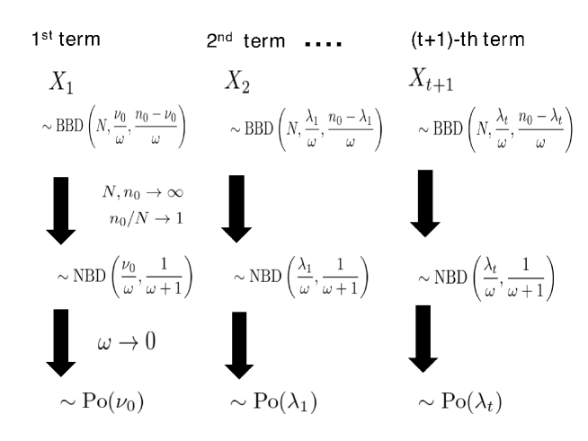
By considering a double-scaling limit, the DT-SE-NBD process can be constructed as an extension of the multi-term Pólya urn process with a memory kernel as follows:
Here, BBD represents the beta-binomial distribution, and the variables represent the number of trials, the number of red balls, and the number of blue balls in an urn in the -th term, respectively. In each term, we sequentially remove a ball and return it along with additional balls of the same color. Consequently, the total number of balls in the urn increases by . The process is repeated times within one term. The term represents Pearson’s correlation coefficient, , which reflects the correlation between the color choices of the balls in the process (Hisakado et al. 2006). The feedback term induces an intertemporal correlation of the ball choices. Furthermore, as approaches zero, under the condition follows a Poisson random variable with a mean of , thereby transforming the DT-SE-NBD process into a DT-SE Poisson process.
Fig.1 illustrates the transformation from the multi-term Pòlya urn process to the DT-SE Negative binomial and DT-SE Poisson process.
We study the (unconditional) expected value of . As for , we have
where is the ensemble average of the stochastic process [i.e., Filtration ]. We are now interested in the steady state of the process and write the unconditional expected value of as . We have the following relationship:
With , and the normalization of the discount factor , we have
We then obtain,
The phase transition between the steady and non-steady state occurs at , which is the critical point. This is the same as that in the Hawkes process. In this sense, corresponds to the branching ratio of the Hawkes process, and the steady-state condition is .
We proceed to the continuous time SE-NBD process. We begin with the DT-SE-NBD process in (1), (2), and (3). The stochastic process is non-Markovian, so we focus on the time evolution of . We decompose as follows:
satisfies the following recursive equation:
Here, we use the relation . The stochastic difference equation for is
| (4) |
The DT-SE-NBD process is now represented by a multivariate stochastic difference equation.
Now, we consider the continuous time limit. We divide the unit time interval by infinitesimal time intervals with width . The decreasing factor for unit time period is replaced by for . In addition, we adopt the notation . Here, we replace the normalization factor of with in to ensure that . We introduce the continuous time memory kernel as
| (5) |
We denote the continuous time limits of and as and , respectively. The timing, size of events, and counting process are denoted by , and , respectively. and are defined as
is the common noise for the time interval in the DT SE-NBD process. To take the continuous time limit, it is necessary to define the noise for the infinitesimal interval . There is freedom in defining , and we adopt the following, which is based on the reproduction properties of NBD. When ,. We define for the interval as
If we consider the above-mentioned noise, by the reproduction property, the noise for the interval becomes
In the self-exciting process, we replace and by and , respectively. The conditional expected value and variance of are
The conditional probability of occurrence of an event with size during the time interval is given as
In the limit , the probabilities converge to
and the event size is restricted to one.
The NBD noise is then written as
The probability mass function (PMF) for event size is given by
| (6) |
The intensity of the process, , is then given as
| (7) |
This process is known as the marked Hawkes process. Each event has a distinct influential power that is encoded in the marks . are IID random numbers and obey the PMF of (6). When the parameter tends to zero (), the PMF approaches the delta function , and the marked Hawkes process reduces to the “pure” Hawkes process. In the following analysis, we will focus on studying the PDF of the intensities in the marked Hawkes process.
3 Solution
The multivariate difference equation (4) can be transformed into a multivariate SDE as follows:
| (8) | |||||
| (9) | |||||
| (10) |
Note that the same state-dependent NBD noise affects every component of the multivariate SDE . In other words, each shock event simultaneously affects the trajectories for all excess intensities .
We adopted the same procedure to derive the master equation for the PDF of in Ref.(Kanazawa and Sornette 2020b, a). As the SDEs for are standard Markovian stochastic processes, we obtain the corresponding master equation
| (11) |
The jump-size vector is given by .
The master equation (3) takes a simplified form under the Laplace representation:
| (12) |
where the Laplace transformation in the -dimensional space is defined as
| (13) |
with the volume element . The wave vector is the conjugate of the excess intensity vector .
The Laplace representation of the master equation (3) is given by
| (14) |
Then, the Laplace representation (12) of , which is the solution of (14), enables us to obtain the (one-dimensional) Laplace representation of the intensity according to
| (15) |
A. Single exponential kernel
We now consider the case in which the memory function (5) consists of exponential functions(Hisakado et al. 2022a). The Laplace representation of the master equation (3) is given by
The steady-state PDF of the intensity is
| (16) |
The power-law exponent of the PDF of the excess intensity is and depends on . In the limit , the result coincides with that in Ref.(Kanazawa and Sornette 2020b, a). The power-law exponent increases with and converges to in the limit . In addition, the length scale beyond which the intensity shows exponential decay for the off-critical case is , and it diverges in the limit . This is also an increasing function of .
B. Double exponential kernel
We consider the case where the memory function (5) consists of exponential functions. To derive the solution for the Laplace representation of the master equation (14), we apply the method of characteristics as in Ref.(Kanazawa and Sornette 2020a). One can find a brief explanation in Refs.(Gardiner 2009) and (Kanazawa and Sornette 2020a). In appendix A, we provide a brief review.
We start from the Lagrange–Charpit equations, which are given by
| (17) | |||||
| (18) | |||||
| (19) |
and is the auxiliary “time” parameterizing the position on the characteristic curve. Let us develop the stability analysis around (i.e., for large ) for this pseudo-dynamical system.
a. Sub-critical case
Assuming , we first expand to compute the sum of :
| (21) |
We obtain the linearized dynamics of the system (17),(18),(19) as follows:
| (22) |
with
We introduce the eigenvalues and eigenvectors of such that
The matrix is the same with the results of Ref.(Kanazawa and Sornette 2020b, a) and all eigenvalues are real. We denote them as . The determinant of is given by
This implies that the zero eigenvalue appears at the critical point . Below the critical point , all eigenvalues are positive (). For , the dynamics can be rewritten as
Here, and are integration constants. We can assume as the initial point of the characteristic curve without loss of generality. Integrating the second equation in (22), we obtain
The general solution is given by
| (23) |
with function determined by the initial condition of the characteristic curve. Let us introduce
This implies that the solution is given in the following form:
Owing to the renormalization of the PDF, the relation
must hold for any path in the () space ending at the origin (). Let us consider a specific limit such that and for an arbitrary positive .
Because the left-hand side is zero for any , the function must be exactly zero. Thus, this leads to
By substituting , we obtain
This is consistent with the asymptotic mean intensity in the steady state (Kanazawa and Sornette 2020b, a).
b. Critical case
In this case, the eigenvalues and eigenvectors of are given by
This means that the eigenvalue matrix and its inverse matrix are given by
Here, let us introduce
| (24) |
We then obtain
at the leading linear order in the expansions of the powers of and . Because the first linear term is zero in the dynamics of , corresponding to a transcritical bifurcation for the Lagrange–Charpit equations (16), we need to consider the second-order term in , namely,
where we dropped the terms of the order , , and . We then obtain the dynamic equations at the transcritical bifurcation to the leading order:
whose solutions are given by
with constants of integration and . We can assume is the initial point on the characteristic curve. Remarkably, only the contribution along the axis is dominant for the large limit (i.e., for ), which corresponds to the asymptotic . We then obtain
with integration constant . is a divergent constant because it has to compensate the diverging logarithm to ensure that . This divergent constant appears as a result of neglecting the ultraviolet (UV) cutoff for small (which corresponds to neglecting the exponential tail of the PDF of intensities) (Kanazawa and Sornette 2020a).
Therefore, we obtain the steady solution
for small and by ignoring the UV cutoff and constant contribution. This recovers the power-law formula of the intermediate asymptotic of the PDF of the Hawkes intensities:
| (25) | |||||
where , as defined in (24). The power-law exponent of the PDF of the excess intensity is and depends on . In the limit , the result coincides with that in Ref.(Kanazawa and Sornette 2020b, a).
C. Discrete superposition of exponential kernels
We now study the case in which the memory kernel is the sum of exponentials for an arbitrary finite number . We obtain the steady-state PDF of the intensity as
| (26) |
The power-law exponent of the PDF of the excess intensity is and depends on . In the limit , the result coincides with that in Ref.(Kanazawa and Sornette 2020b, a).
D. General case
We study the case where the memory kernel is a continuous superposition of exponential functions. We decompose the kernel as
This decomposition satisfies the normalization condition . The function quantifies the contribution of the exponential kernel to the branching ratio. The steady-state PDF of the intensity is
| (27) |
The power-law exponent of the PDF of the excess intensity is and depends on . In the limit , the result coincides with that in Ref.(Kanazawa and Sornette 2020b, a).
We now consider the case in which the memory kernel exhibits power-law decay. We express as the superposition of with the weight of the gamma distribution as
By the change of variable , we rewrite as the superposition of with the weight of the inverse gamma distribution as
| (28) |
of Eq.(27) is obtained as the expected value of the inverse gamma distribution,
| (29) |
The power-law exponent is .
4 Numerical verification
We conducted numerical simulations to study the steady-state PDF of the intensity in the marked Hawkes process. In particular, our goal was to verify the theoretical predictions of Eqs. (16), (25), (26), and (29). We employed the time-rescaling theorem, which enables us to sample data more efficiently than the rejection method. The time-rescaling theorem states that any point process with an integrable conditional intensity function can be transformed into a Poisson process with a unit rate (Brown et al. 2002). That is, it is possible to convert a marked Hawkes process into a marked point process with a constant intensity of 1 by performing time-dependent rescaling. A point process with intensity 1 can easily generate the time of the next event occurrence because the event interval follows an exponential distribution. The time-rescaling theorem introduces the following time transformations:
| (30) |
When event follows a marked Hawkes process with intensity function in the observation interval , event obtained by the time transformation (30) follows a marked point process with intensity in the observation interval . The event interval is given by
Hence, to numerically realize the marked Hawkes process, it is sufficient to generate a random number following an exponential distribution with mean 1 and successively find that satisfies the above relation.
We rewrite the relation more concretely. For , is written as
The integral of is
We have to solve the next relation,
| (31) | |||||
Note that the jump size of this process is determined according to the distribution of the mark in Eq.(6) when the event occurrence time is determined. The numerical procedures are given below.
We denote .
We performed numerical simulations using Julia 1.7.3. The simulation time for is approximately 0.5 h for background intensity and . The execution environment is as follows: OS: Ubuntu 20.045 LTS, Memory: 64 GB, CPU: 4.7 GHz. The code is available on github(Sakuraba 2023). We sampled the point process with . The common settings of the sampling processes are and .
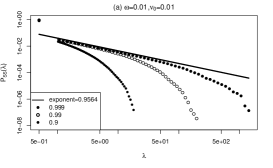
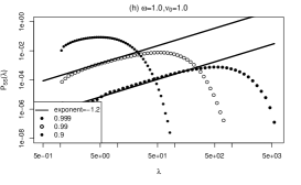
a. Single exponential kernel
 |
 |
 |
 |
 |
 |
 |
 |
 |
For a small background intensity , the power-law exponents are and for and , respectively. These exponents are close to 1 and show little dependence on . For large , the power-law exponent becomes more dependent on . When , the power-law exponents are and for and , respectively. When , The power-law exponent becomes universally 1, as the expression holds. Furthermore, the length scale of the power-law region, denoted as , increases as increases. The numerical results confirm these findings by demonstrating agreement between the slopes of the PDFs and the theoretical values, and the exponents of the power-law were verified. In addition, by observing the -axis, it can be seen that the range of the straight power-law region becomes wider as increases.
b. Double exponential kernel
We verified the theoretical predictions of Eq. (25).
To realize , we set and . Fig.3 presents the double logarithmic plot of PDFs of . One can observe the agreement between the slopes of the PDFs and the theoretical values and the theoretical prediction is verified.
 |
 |
 |
 |
 |
 |
 |
 |
 |
c. Triple exponential kernel
We verified the theoretical predictions of Eq. (26) for .
To achieve , we set , and . Fig.4 shows the resulting PDFs of . One can observe the agreement between the slopes of the PDFs and the theoretical values and the theoretical prediction is verified.
 |
 |
 |
 |
 |
 |
 |
 |
 |
d. Power-law memory kernel
We verified the theoretical predictions of Eq.(29) for .
As in (28), we set and as the % point of the distribution. To achieve , we set . Fig.5 illustrates the resulting PDFs of , confirming the validity of the theoretical prediction for .
 |
 |
 |
 |
 |
 |
 |
 |
 |
5 Conclusion
Here, we investigated the continuous time self-exciting negative binomial process with a memory kernel consisting of a sum of finite exponential functions. This process is equivalent to the marked Hawkes process. Our aim was to extend the previous findings on the intermediate power-law behavior of the intensities near the critical point for the steady and non-steady state phase transition to the case of . To achieve this, we developed an efficient sampling method for the marked Hawkes process based on the time-rescaling theorem. We conducted extensive simulations, focusing specifically on the scenario where to capture the process with a power-law memory kernel. Through these simulations, we were able to verify the theoretical predictions and confirm their accuracy.
Appendix A Method of Characteristics
The method of characteristics is a standard method to solve first-order partial differential equations (Gardiner 2009, Kanazawa and Sornette 2020b, a). The equation for the characteristic function
is
| (A.1) |
We consider the corresponding Lagrange–Charpit equations
with the parameter encoding the position along the characteristic curves. These equations are equivalent to an invariant form in terms of
The method of characteristics can be used to solve this equation. Namely, if
are two integrals of the subsidiary equation (with and arbitrary constants), then a general solution of (A.1) is given by
Appendix B Addendum
In a recent publication by K.Kanazawa and D.Sornette (Kanazawa and Sornette 2023), the power-law exponent of the intensity distribution of general marked Hawkes process was given. We explain the correspondence for the reader’s convenience.
In (Kanazawa and Sornette 2023), the power-law exponent is given using the second moment of the mark’s PDF E as
The normalization of with E is adopted. In our model, is given as
We use in Eq.(6) to estimate the power-law exponent. As E, E, we obtain
The result is consistent with ours in (Hisakado et al. 2022a).
Acknowledgements.
This work was supported by JPSJ KAKENHI [Grant No. 22K03445]. We would like to thank Editage (www.editage.com) for English language editing.References
- Bacry et al. (2015) Bacry E, Mastromatteo I, Muzy J (2015) Hawkes processes in finance. market microstructure and liquidity, 1, 1550005
- Blanc et al. (2017) Blanc P, Donier J, Bouchaud JP (2017) Quadratic hawkes processes for financial prices. Quantitative Finance 17(2):171–188
- Bowsher (2007) Bowsher CG (2007) Modelling security market events in continuous time: Intensity based, multivariate point process models. Journal of Econometrics 141(2):876–912
- Brown et al. (2002) Brown EN, Barbieri R, Ventura V, Kass RE, Frank LM (2002) The time-rescaling theorem and its application to neural spike train data analysis. Neural computation 14(2):325–346
- Engle and Russell (1998) Engle RF, Russell JR (1998) Autoregressive conditional duration: a new model for irregularly spaced transaction data. Econometrica pp 1127–1162
- Errais et al. (2010) Errais E, Giesecke K, Goldberg LR (2010) Affine point processes and portfolio credit risk. SIAM Journal on Financial Mathematics 1(1):642–665
- Filimonov and Sornette (2012) Filimonov V, Sornette D (2012) Quantifying reflexivity in financial markets: Toward a prediction of flash crashes. Physical Review E 85(5):056108
- Filimonov and Sornette (2015) Filimonov V, Sornette D (2015) Apparent criticality and calibration issues in the hawkes self-excited point process model: application to high-frequency financial data. Quantitative Finance 15(8):1293–1314
- Gardiner (2009) Gardiner C (2009) Stochastic Methods A Handbook for the Natural and Social Sciences. Springer, Berlin
- Hasbrouck (1991) Hasbrouck J (1991) Measuring the information content of stock trades. The Journal of Finance 46(1):179–207
- Hawkes (1971a) Hawkes A (1971a) Point spectra of some mutually exciting point processes. Journal of the Royal Statistical Society Series B 33, DOI 10.1111/j.2517-6161.1971.tb01530.x
- Hawkes (1971b) Hawkes AG (1971b) Spectra of some self-exciting and mutually exciting point processes. Biometrika 58(1):83–90
- Hawkes (2018) Hawkes AG (2018) Hawkes processes and their applications to finance: a review. Quantitative Finance 18(2):193–198
- Hawkes and Oakes (1974) Hawkes AG, Oakes D (1974) A cluster process representation of a self-exciting process. Journal of Applied Probability 11(3):493–503
- Hisakado and Mori (2020) Hisakado M, Mori S (2020) Phase transition in the bayesian estimation of the default portfolio. Physica A: Statistical Mechanics and its Applications 544:123480
- Hisakado et al. (2006) Hisakado M, Kitsukawa K, Mori S (2006) Correlated binomial models and correlation structures. Journal of Physics A: Mathematical and General 39(50):15365
- Hisakado et al. (2022a) Hisakado M, Hattori K, Mori S (2022a) From the multiterm urn model to the self-exciting negative binomial distribution and hawkes processes. Physical Review E 106(3):034106
- Hisakado et al. (2022b) Hisakado M, Hattori K, Mori S (2022b) Multi-dimensional self-exciting nbd process and default portfolios. The Review of Socionetwork Strategies 16(2):493–512
- Kanazawa and Sornette (2020a) Kanazawa K, Sornette D (2020a) Field master equation theory of the self-excited hawkes process. Physical Review Research 2(3):033442
- Kanazawa and Sornette (2020b) Kanazawa K, Sornette D (2020b) Nonuniversal power law distribution of intensities of the self-excited hawkes process: A field-theoretical approach. Physical Review Letters 125(13):138301
- Kanazawa and Sornette (2023) Kanazawa K, Sornette D (2023) Asymptotic solutions to nonlinear hawkes processes: A systematic classification of the steady-state solutions. Physical Review Research 5(1):013067
- Kirchner (2017) Kirchner M (2017) An estimation procedure for the hawkes process. Quantitative Finance 17(4):571–595
- Sakuraba (2023) Sakuraba K (2023) Self-exciting negative binomial distribution process and critical properties of intensity distribution. URL https://github.com/Kotaro-Sakuraba/SE-NBD_Process.git
- Wheatley et al. (2019) Wheatley S, Wehrli A, Sornette D (2019) The endo–exo problem in high frequency financial price fluctuations and rejecting criticality. Quantitative Finance 19(7):1165–1178