Self-Attentive 3D Human Pose and Shape Estimation from Videos
4.5 Run-time analysis
We report the model training time in hours, the inference time for processing an image in seconds, and the GPU platform used by each method in Table 6. First, the training time of our method is shorter than that of the HMR (Kanazawa et al., 2018), STRAPS (Sengupta et al., 2020), and HUND (Zanfir et al., 2020). Second, the inference time of our method is comparable to that of the VIBE method (Kocabas et al., 2020), and shorter than that of the ExPose (Choutas et al., 2020) and STRAPS (Sengupta et al., 2020) approaches. Third, our method performs favorably against existing frame-based and video-based approaches on all three datasets as shown in Table 1.
Abstract
We consider the task of estimating 3D human pose and shape from videos. While existing frame-based approaches have made significant progress, these methods are independently applied to each image, thereby often leading to inconsistent predictions. In this work, we present a video-based learning algorithm for 3D human pose and shape estimation. The key insights of our method are two-fold. First, to address the inconsistent temporal prediction issue, we exploit temporal information in videos and propose a self-attention module that jointly considers short-range and long-range dependencies across frames, resulting in temporally coherent estimations. Second, we model human motion with a forecasting module that allows the transition between adjacent frames to be smooth. We evaluate our method on the 3DPW, MPI-INF-3DHP, and Human3.6M datasets. Extensive experimental results show that our algorithm performs favorably against the state-of-the-art methods.
keywords:
MSC:
41A05, 41A10, 65D05, 65D17 \KWD3D human pose and shape estimation , Self-supervised learning , Occlusion handling1 Introduction
3D human pose and shape estimation (Kanazawa et al., 2018; Kolotouros et al., 2019a; Bogo et al., 2016) is an active research topic in computer vision and computer graphics that finds numerous applications (Xu et al., 2019; Liu et al., 2019). The inherent under-constrained nature where multiple 3D meshes can explain the same 2D projection makes this problem very challenging. While frame-based methods (Kanazawa et al., 2018; Kolotouros et al., 2019a; Bogo et al., 2016) and video-based approaches (Kocabas et al., 2020; Lee et al., 2018b; Rayat Imtiaz Hossain and Little, 2018; Kanazawa et al., 2019; Zhang et al., 2019b) have been developed to recover human pose in the literature, numerous issues remain to be addressed. First, existing approaches employ recurrent neural networks (RNNs) to model temporal information for consistent predictions. However, it is difficult to train RNNs to capture long-range dependencies (Vaswani et al., 2017; Pascanu et al., 2013). On the other hand, one recent approach employing RNNs does not consistently render smooth predictions across frames (Kocabas et al., 2020).
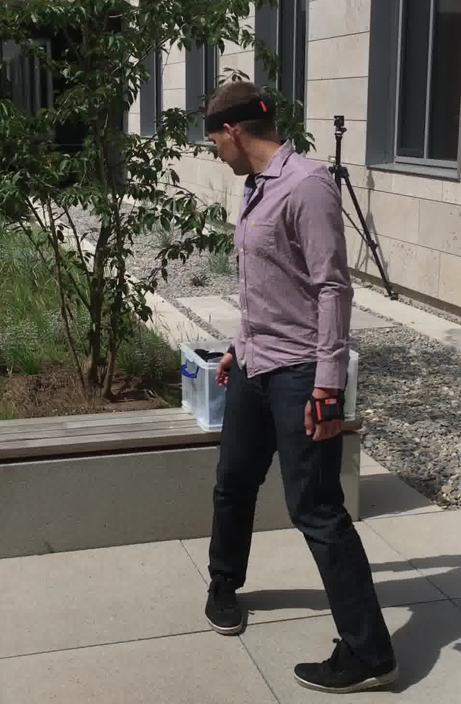
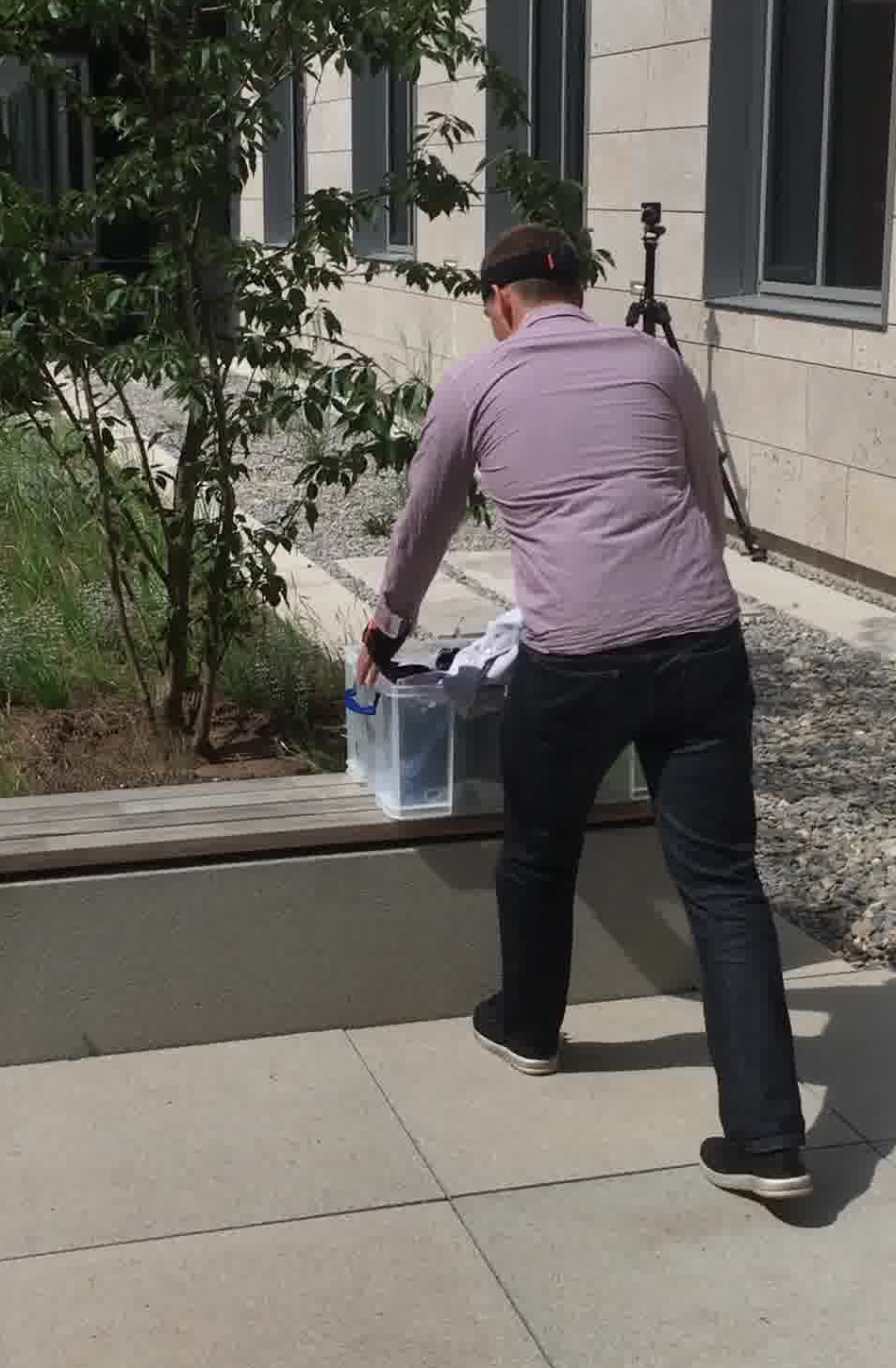
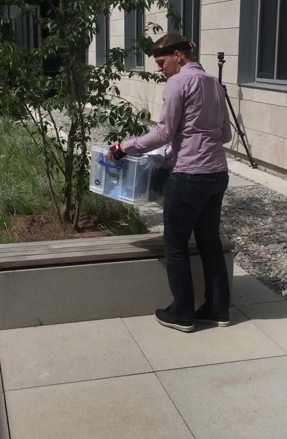
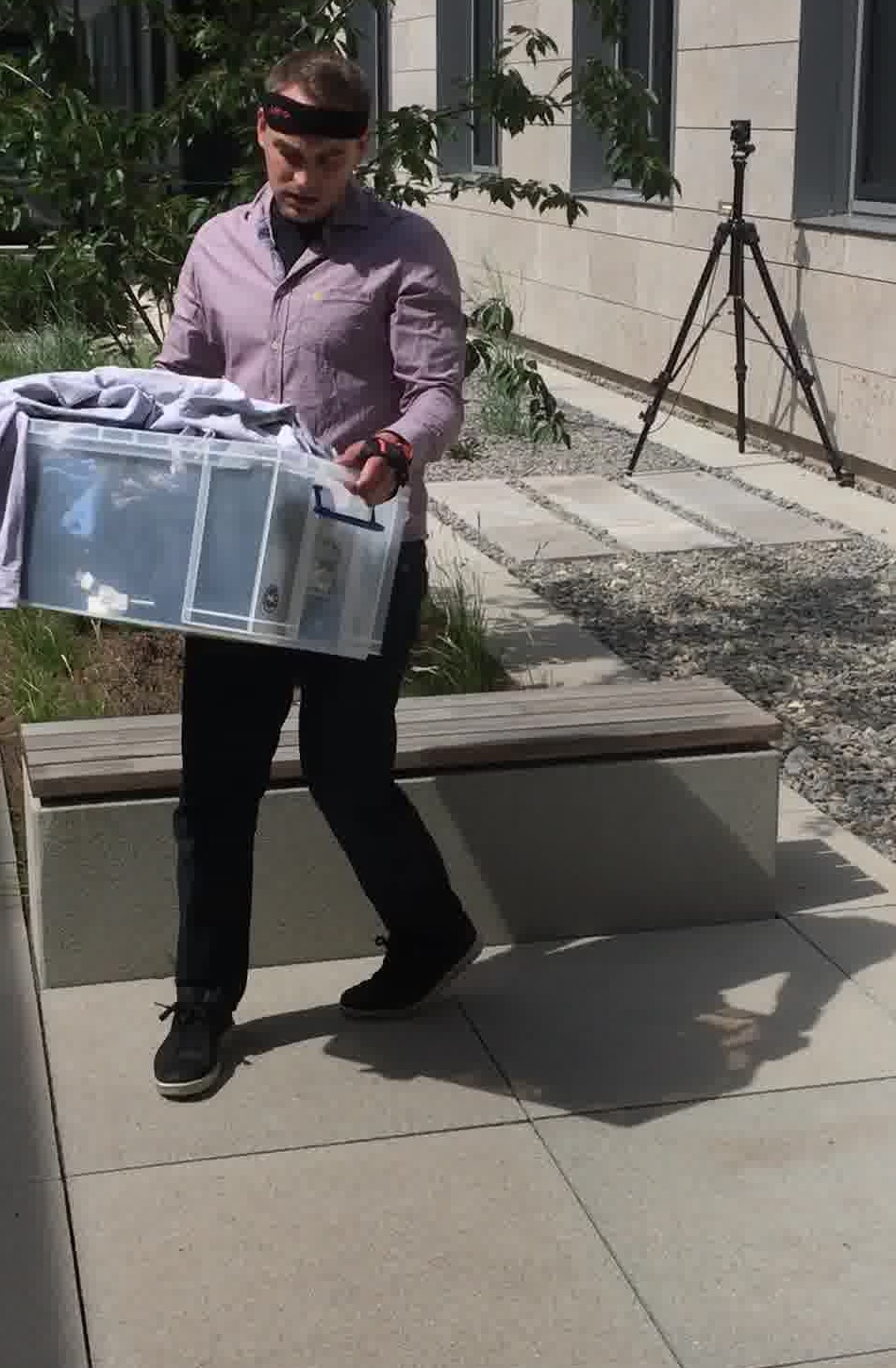
[autoplay,loop,width=]30gif/000000000234
Second, as most real-world datasets do not contain ground-truth camera parameter annotations, existing methods typically reproject the predicted 3D joints onto the 2D space using the estimated camera parameters, followed by a loss enforced between the reprojected 2D joints and the corresponding ground-truth 2D joints. Nevertheless, such regularization terms are still insufficient to account for complex scenes. Third, existing methods (Kocabas et al., 2020; Kanazawa et al., 2019; Zhang et al., 2019b; Kanazawa et al., 2018) do not perform well for humans under heavy occlusion or out-of-view, as there is no explicit constraint enforced on the invisible regions.
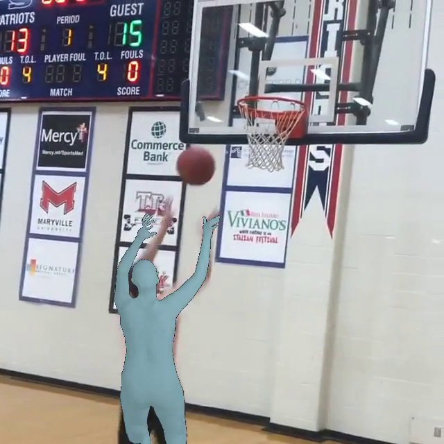
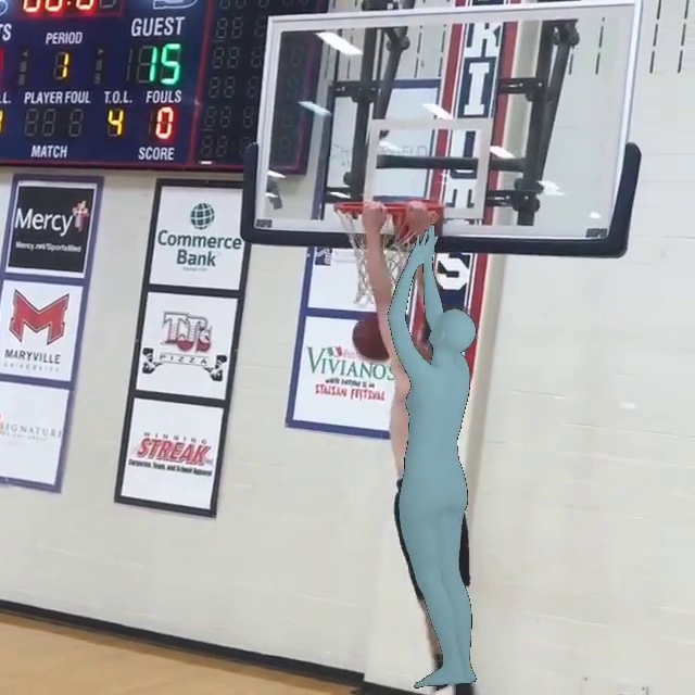
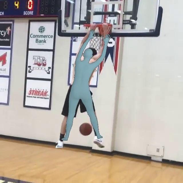
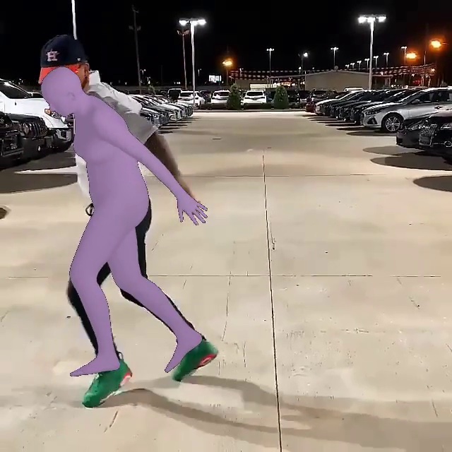
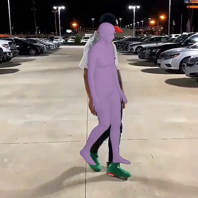
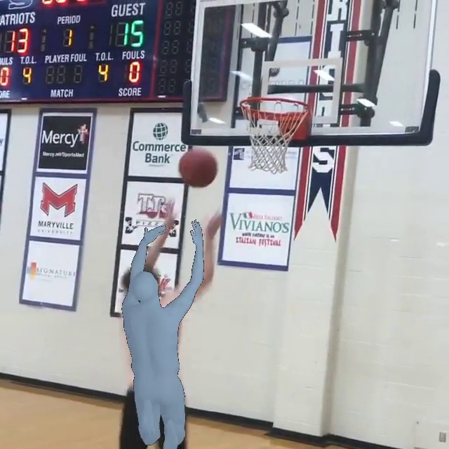
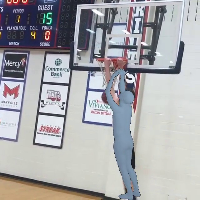
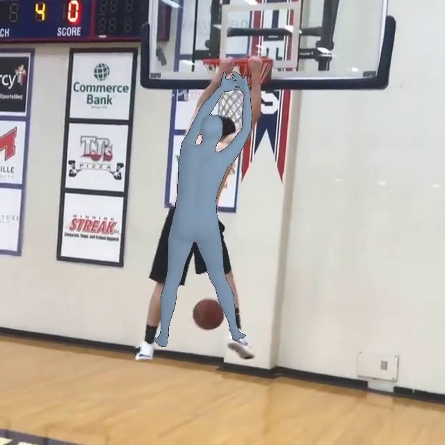
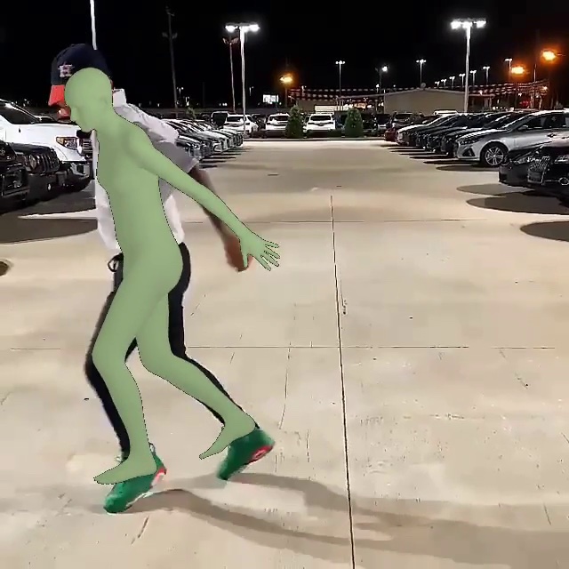
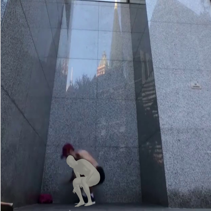
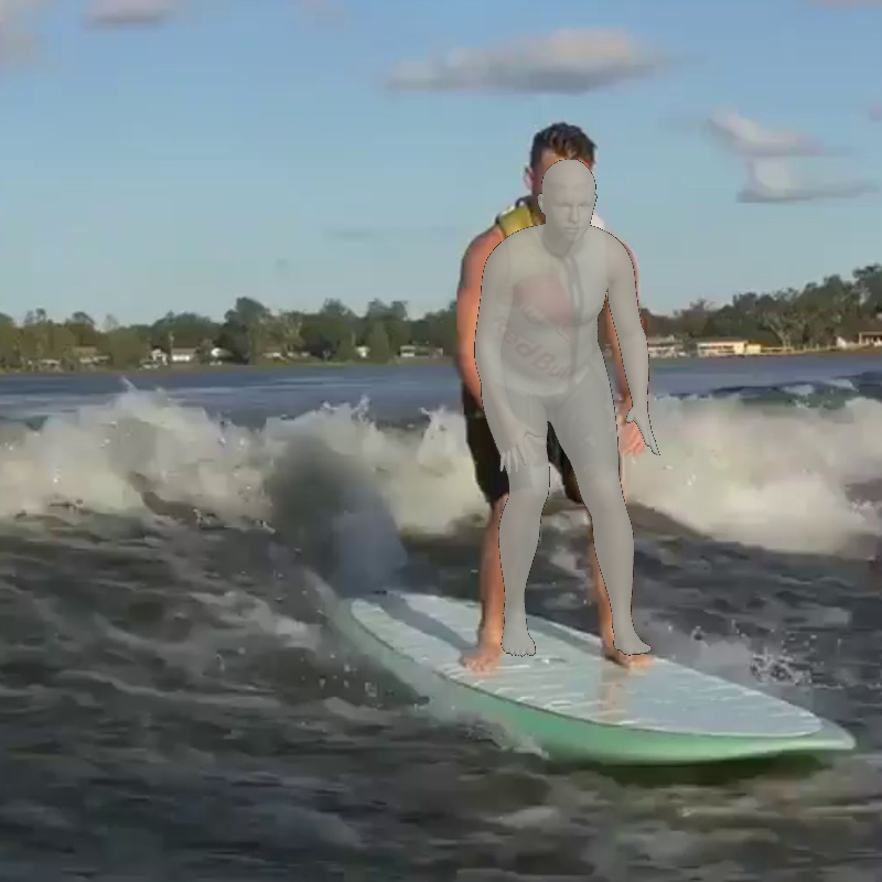
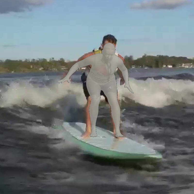
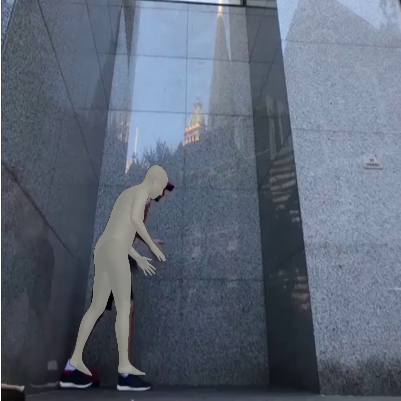
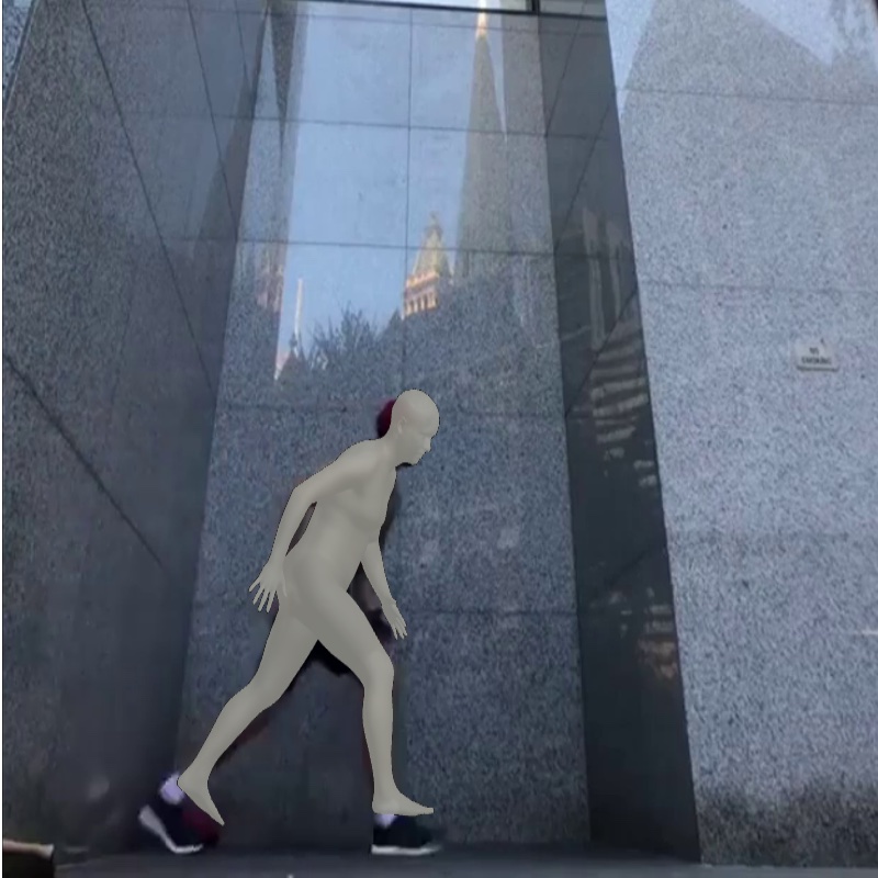
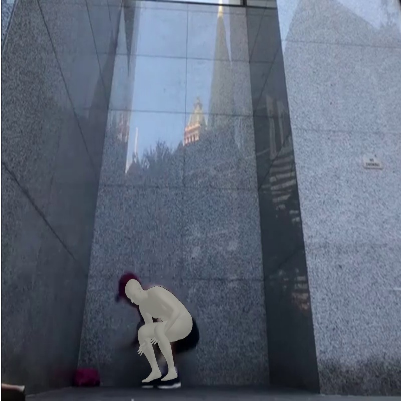
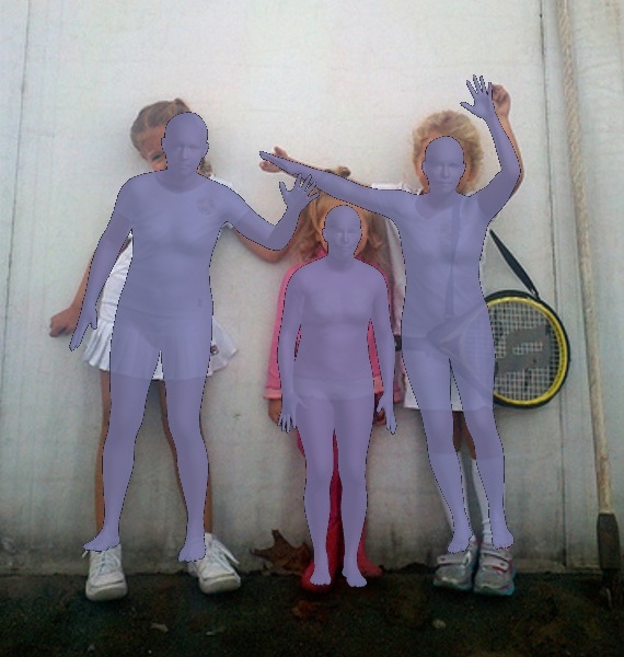
In this paper, we propose the Self-attentive Pose and Shape Network (SPS-Net) for 3D human pose and shape estimation from videos. Our key insights are two-fold. First, motivated by the attention models in neural machine translation (Vaswani et al., 2017) and image generation (Zhang et al., 2019a) tasks, we develop a self-attention module to exploit temporal cues in videos for coherent predictions. For each input frame, our self-attention module derives a visual representation by observing past and future frames and predicting the associated attention weights. Second, motivated by the autoregressive models in human motion prediction (Kanazawa et al., 2019; Zhang et al., 2019b), we develop a forecasting module that leverages visual cues from human motion to encourage our model to generate temporally smooth predictions. By jointly considering both features, our SPS-Net is able to estimate accurate and temporally coherent human pose and shape (see Figure 1).
To account for images without ground-truth camera parameter annotations, we exploit the property that the camera parameters for the overlapped frames of two segments from the same video should be the same. We enforce this constraint with a camera parameter consistency loss. Furthermore, we address the occlusion and out-of-view issues by masking out some regions of the video frames. Our core idea is to leverage the predictions of the original video frames to supervise those of the synthesized occluded or partially visible data, making our model more robust to the occlusion and out-of-view issues. We demonstrate the effectiveness of the proposed SPS-Net on three standard benchmarks, including the 3DPW (von Marcard et al., 2018), MPI-INF-3DHP (Mehta et al., 2017a), and Human3.6M (Ionescu et al., 2013) datasets.
Our main contributions can be summarized as follows:
-
•
We present a video-based learning algorithm for 3D human pose and shape estimation.
-
•
We propose a camera parameter consistency loss that provides additional supervisory signals for model training, resulting in more accurate camera parameter predictions.
-
•
Our model learns to predict plausible estimations when occlusion or out-of-view occurs in a self-supervised fashion.
-
•
Extensive evaluations on three challenging benchmarks demonstrate that our method achieves the state-of-the-art performance against existing approaches.
2 Related Work
3D human pose and shape estimation. Existing methods for 3D human pose and shape estimation can be broadly categorized as frame-based and video-based. Frame-based methods typically use an off-the-shelf keypoint detector (e.g., DeepCut (Pishchulin et al., 2016)) to fit the SMPL (Loper et al., 2015) body model (Bogo et al., 2016), leverage silhouettes and keypoints for model fitting (Lassner et al., 2017), or directly regress the parameters for the SMPL (Loper et al., 2015) body model from pixels using neural networks (Kolotouros et al., 2019a; Kanazawa et al., 2018; Kolotouros et al., 2019b). While these frame-based approaches are able to recover 3D poses from a single image, independently applying these algorithms to each video frame often leads to temporally inconsistent predictions. Video-based methods, on the other hand, usually adopt RNN-based models to generate temporally coherent predictions. These approaches either focus on estimating the human body of the current frame (Arnab et al., 2019; Sun et al., 2019; Kocabas et al., 2020) or predicting the past and future motions (Kanazawa et al., 2019; Zhang et al., 2019b).
Our algorithm differs from these video-based methods in three aspects. First, in contrast to adopting RNN-based models, we develop a self-attention module to aggregate temporal information and a forecasting module to model human motion for predicting temporally coherent estimations. Second, we enforce a consistency loss on the prediction of camera parameters to regularize model learning. Third, we address the occlusion and out-of-view issues with a self-supervised learning scheme to generate plausible human pose and shape predictions.
Attention models. Attention models have been shown effective in neural machine translation (Vaswani et al., 2017) and image generation problems (Zhang et al., 2019a; Parmar et al., 2018). For machine translation, employing self-attention models (Vaswani et al., 2017) helps capture short-range and long-range correlations between tokens in the sentence for improving the translation quality. In image generation, the Image Transformer (Parmar et al., 2018) and SAGAN (Zhang et al., 2019a) show that leveraging self-attention mechanisms facilitates the models to generate realistic images. In 3D human pose and shape estimation, the VIBE (Kocabas et al., 2020) method adopts a self-attention scheme in the discriminator for feature aggregation, allowing the discriminator to better distinguish the motions of attended video frames between the real sequences and generated ones.
We adopt self-attention modules in both the SPS-Net and discriminator. Our method differs from the VIBE (Kocabas et al., 2020) in that our self-attention module aims to derive a representation for each frame that contains temporal information by jointly considering short-range and long-range dependencies across video frames, whereas the VIBE (Kocabas et al., 2020) method aims to derive a single representation for the entire pose sequence.
Future human pose predictions. Predicting future poses from videos has been studied by a few approaches in the literature. Existing algorithms estimate 2D poses from pixels (Denton and Birodkar, 2017; Finn et al., 2016), optical flow (Walker et al., 2016), or 2D poses (Walker et al., 2017), or predict 3D outputs based on 3D inputs (Butepage et al., 2017; Fragkiadaki et al., 2015; Jain et al., 2016; Li et al., 2018; Villegas et al., 2018). Other approaches learn 3D pose prediction from 2D inputs (Zhang et al., 2019b; Kanazawa et al., 2019).
Similar to the HMMR (Kanazawa et al., 2019) and PHD (Zhang et al., 2019b) methods, we leverage visual cues from human motion to predict temporally smooth predictions. Our method differs from them in that our self-attention module helps capture short-range and long-range dependencies across video frames in the input video, while the 1D convolution in the temporal encoder and autoregressive module of these methods does not have such ability.
Consistency constraints for visual learning. Exploiting consistency constraints to regularize model learning has been shown effective in numerous applications, including semantic matching (Zhou et al., 2015), optical flow estimation (Meister et al., 2018), depth prediction (Gordon et al., 2019), and image-to-image translation (Zhu et al., 2017; Lee et al., 2018a; Huang et al., 2018). Other methods exploit consistency constraints across multiple network outputs, including depth and optical flow estimation (Zou et al., 2018), joint semantic matching and object co-segmentation (Chen et al., 2020), ego-motion (Zhou et al., 2017), and domain adaptation (Chen et al., 2019b). In our work, we show that enforcing consistency constraints on the prediction of camera parameters for the overlapped video frames of two segments from the same video results in performance improvement.
3 Proposed Algorithm
In this section, we first provide an overview of our approach. Next, we describe the details of the self-attention and forecasting modules, followed by formulating the proposed camera parameter consistency loss. We then motivate the self-supervised learning scheme for addressing the occlusion and out-of-view issues.
3.1 Algorithmic overview
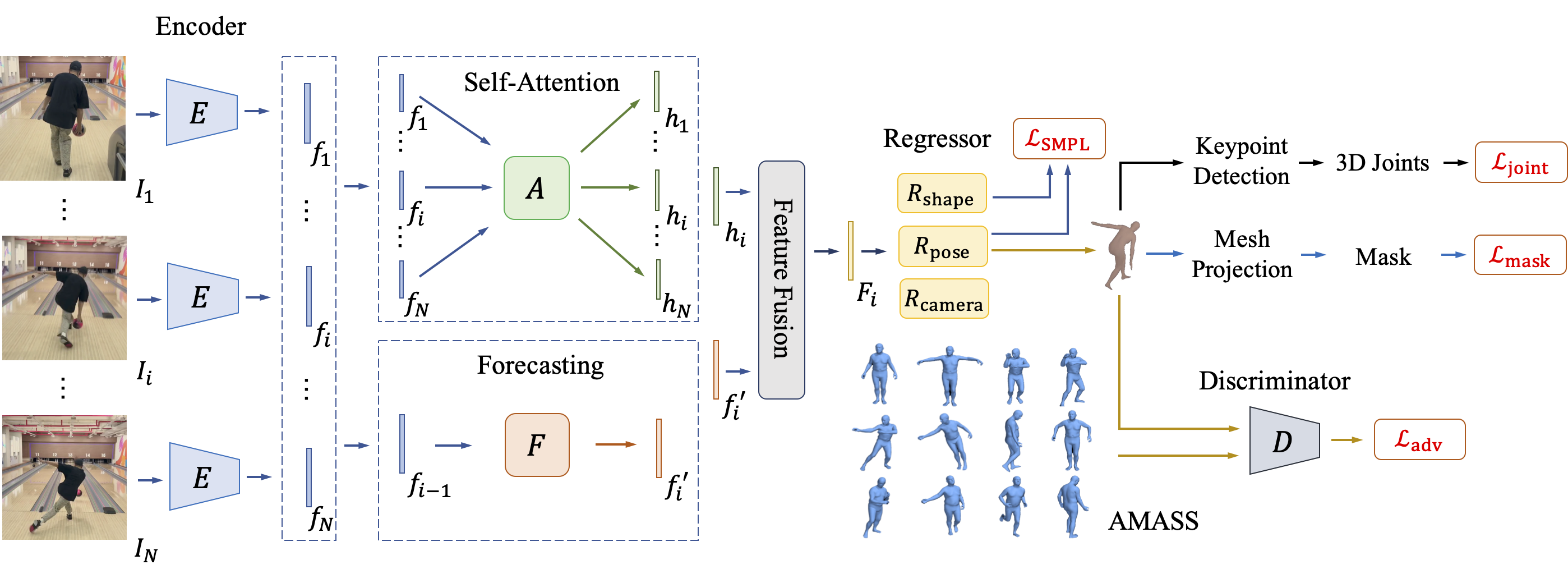
Given an input video of length containing a single person, our goal is to learn a model that recovers the 3D human body of each frame. We present the Self-attentive Pose and Shape Network (SPS-Net), comprising four components: 1) feature encoder , 2) self-attention module , 3) forecasting module , and 4) three parameter regressors , , and .
As shown in Figure 2, we first apply the encoder to each frame to extract the feature , where denotes the number of channels of the feature . Next, the self-attention module takes all the encoded features as input and outputs the corresponding latent representations , where denotes the latent representation for , containing temporal information of past and future frames. The forecasting module takes each encoded feature as input and forecasts the feature of the next time step . The latent representations and the predicted features of the same time step (e.g., and ) are passed to a feature fusion module to derive the fused representations , where contains both global temporal and local motion information. The pose parameter regressor takes each fused representation as input and renders the pose parameters for each frame , where . The shape parameter regressor , on the other hand, takes all the fused representations as input and regresses the shape parameters of the input video .
3D human body representation. Similar to the state-of-the-art methods (Kanazawa et al., 2018; Kolotouros et al., 2019a; Kocabas et al., 2020), we adopt the SMPL (Loper et al., 2015) body model to describe the human body using a 3D mesh representation. The SMPL (Loper et al., 2015) model is described by the pose and shape parameters. The pose parameters contain the global body rotation and the relative 3D rotation of joints in axis-angle format. The shape parameters are parameterized by the first linear coefficients of a PCA shape space. We use a gender-neutral shape model as in previous work (Kanazawa et al., 2018; Kolotouros et al., 2019a; Kocabas et al., 2020). The differentiable SMPL (Loper et al., 2015) body model takes the pose and shape parameters as input and outputs a triangular mesh consisting of mesh vertices by shaping a template body mesh based on forward kinematics. The 3D keypoints of body joints can be obtained by applying a pre-trained linear regressor to the 3D mesh , and is defined as .
Camera model. Similar to existing approaches (Kanazawa et al., 2018; Kolotouros et al., 2019a; Kocabas et al., 2020), we use a weak-perspective camera model in this work. By estimating the camera parameters using the regressor , where denotes the scale, is the global rotation in axis-angle format, and denotes the translation, the 2D projection of the 3D keypoints can be obtained by , where is an orthographic projection.
3.2 Self-attention module
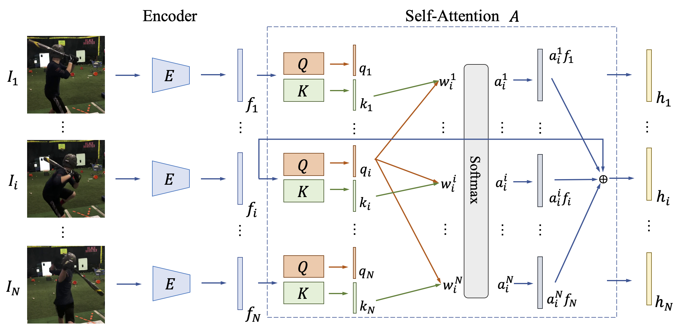
Given a sequence of features encoded by the encoder , our goal is to leverage temporal cues in the input video to provide more information that helps regularize the estimation of human pose and shape. Existing methods exploit temporal information by resorting to an RNN-based model, e.g., GRU (Kocabas et al., 2020) or LSTM (Lee et al., 2018b; Rayat Imtiaz Hossain and Little, 2018). However, training RNN-based models is difficult to capture long-range dependencies (Vaswani et al., 2017; Pascanu et al., 2013).
Motivated by the attention models (Vaswani et al., 2017; Zhang et al., 2019a; Parmar et al., 2018) which have been shown effective to jointly capture short-range and long-range dependencies while being more parallelizable to train (Vaswani et al., 2017), we develop a self-attention module to learn latent representations that jointly observe past and future video frames for producing temporally consistent pose and shape predictions.
The attention weights are computed by
| (1) |
We then apply a weighted sum layer to sum over all input features with the associated attention weights . In addition, we add a residual connection (He et al., 2016) to pass the input feature to the output of the self-attention module. Specifically, the latent representation is described by
| (2) |
3.3 Forecasting module
In addition to considering global temporal information as in the self-attention module , we exploit visual cues from human motion to encourage our model to generate temporally smooth predictions. Motivated by methods that focus on tackling human motion prediction (Kanazawa et al., 2019; Zhang et al., 2019b), we develop a forecasting module that takes each encoded feature as input and forecasts the feature of the next time step . As the feature of the next time step is available (given by the encoder), we train the forecasting module in a self-supervised fashion with a feature regression loss:
| (3) |
We note that since the feature of the next time step of is not available, we do not compute the feature regression loss on .
3.4 3D human pose and shape estimation
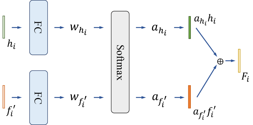
To jointly consider the latent representations that contain global temporal information and the predicted features that contain local motion information for predicting the parameters for 3D human pose and shape estimation, we have a feature fusion module that fuses and at the same time step to derive the fused representations . We note that since our encoder is pre-trained on single-image pose and shape estimation task and fixed during training as in prior work (Kanazawa et al., 2018; Kocabas et al., 2020), the feature encoded by the encoder is static and does not contain motion information. Therefore, we use the predicted feature from the forecasting module that contains motion information for feature fusion.
As shown in Figure 4, our feature fusion module is composed of a fully connected (FC) layer, followed by a softmax layer. Given a latent representation and a predicted feature , we first apply the FC layer to each input feature to predict a weight. The predicted weights are then normalized using a softmax layer. The two input features are then fused by . We note that since is not available, we define .
Next, we pass all the fused features to the shape , pose , and camera parameter regressors to predict the corresponding parameters, respectively. Similar to one prior work (Kanazawa et al., 2018), we adopt an iterative error feedback scheme to regress the parameters. To train the proposed SPS-Net, we impose a SMPL parameter regression loss on the estimated pose and shape parameters, a 3D joint loss on the predicted 3D joints , and a 2D joint loss on the reprojected 2D joints (Kanazawa et al., 2018; Kocabas et al., 2020). Specifically, the SMPL parameter regression loss , the 3D joint loss , and the 2D joint loss are defined as
| (4) |
Mask loss. Since the ground-truth pose , shape , and 3D joint annotations are usually not available, using the 2D joint loss alone is insufficient to train the SPS-Net as there are numerous 3D meshes that can explain the same 2D projection. To address this issue, we exploit the idea that the reprojection of the 3D mesh using the estimated camera parameters should be consistent with the segmentation mask obtained by directly segmenting the human from the input video frame. We leverage an off-the-shelf instance segmentation model (Bolya et al., 2019) to compile a pseudo ground-truth segmentation mask for each input video frame .111We note that while other existing instance segmentation models can also be used for compiling segmentation masks, we leave the discussion of adopting different instance segmentation models as future work. Then, we use the pseudo ground-truth segmentation mask to supervise the reprojection of the 3D mesh with a mask loss:
| (5) |
where denotes the reprojection of the 3D mesh using the estimated camera parameters.
Camera parameter consistency loss. Since there are no ground-truth camera parameter annotations for most datasets, existing methods (Kocabas et al., 2020; Kanazawa et al., 2018; Kolotouros et al., 2019a) regularize the estimation of camera parameters via reprojecting the detected 3D keypoints onto 2D space and enforcing a 2D joint loss between the reprojected 2D joints and the corresponding ground-truth 2D joints. This weaker form of supervision, however, is still under-constrained. To address the absence of ground-truth camera parameter annotations, we exploit the idea that the overlapped video frames in different sequence segments from the same video should have the same camera parameter predictions. Given two input sequence segments and from the same video , the overlapped frames are . We enforce the camera parameter predictions of the overlapped frames to be the same in these two input sequence segments and . To achieve this, we propose a camera parameter consistency loss which is defined as
| (6) |
where and are the fused feature of frame and frame , respectively. Incorporating such consistency loss during training not only regularizes the prediction of camera parameters but also provides more supervisory signals to facilitate model training.
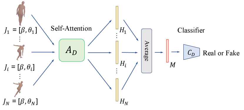
Adversarial loss. In addition to the aforementioned loss functions, we also adopt an adversarial learning scheme that aims to encourage our method to recover a sequence of 3D meshes with realistic motions (Kocabas et al., 2020). Similar to the VIBE (Kocabas et al., 2020) method, we adopt the AMASS (Mahmood et al., 2019) dataset and employ a discriminator that takes as input a sequence of pose parameters with the associated shape parameters estimated by the SPS-Net (treated as a fake example) and a sequence of those sampled from the AMASS (Mahmood et al., 2019) dataset (treated as a real example), and aims to distinguish whether the input sequences are realistic or not.
As shown in Figure 5, our discriminator is composed of a self-attention module and a classifier . We first concatenate the estimated shape parameters with each of the estimated pose parameters to form the joint representations , where . We then pass all joint representations to the self-attention module to derive the latent representations , where is the latent representation of . To derive the motion representation of , we average all the latent representations , i.e., . The motion representation of can be derived similarly. The classifier takes the motion representations and as input and distinguishes whether the input motion representations are realistic or not. Specifically, we have an adversarial loss which is defined as
| (7) |
Leveraging the unpaired data from the AMASS (Mahmood et al., 2019) dataset serves as a weak supervision to encourage the SPS-Net to recover a sequence of 3D meshes with realistic motions.
We note that our discriminator is different from that of the VIBE (Kocabas et al., 2020) method in two aspects. First, our discriminator has a self-attention module, while the discriminator of the VIBE (Kocabas et al., 2020) method has two GRU layers. Second, we use self-attention to derive a representation for each frame that contains temporal information by jointly considering short-range and long-range dependencies across video frames, whereas the VIBE (Kocabas et al., 2020) method leverages self-attention to derive a single representation for the entire pose sequence.
Self-supervised occlusion handling. While the aforementioned loss functions regularize the learning of the SPS-Net, the 2D and 3D joint losses and the mask loss are only enforced on the visible keypoints and regions of the human body. That is, there is no explicit constraint imposed on the invisible keypoints and regions. We develop a self-supervised learning scheme to allow our model to produce plausible predictions in order to account for the occlusion and out-of-view scenarios. For each input frame , we first synthesize the occluded version by randomly masking out some regions. We then leverage the predictions of the original frames to supervise those of the synthesized occluded or partially visible frames and develop a self-supervised parameter regression loss to exploit this property with
| (8) |
By simulating the occlusion and out-of-view scenes, our model is able to predict plausible shape, pose, and camera parameters from the occluded or partially visible frames.
4 Experimental Results
In this section, we first describe the implementation details. Next, we describe the datasets for model training and testing, followed by the evaluation metrics. We then present the quantitative and visual comparisons to existing methods as well as the ablation study.
4.1 Implementation details
We implement our model using PyTorch (Paszke et al., 2019). Same as prior work (Kanazawa et al., 2018; Kocabas et al., 2020), we adopt the ResNet- (He et al., 2016) pre-trained on single-image pose and shape estimation task (Kanazawa et al., 2018; Kolotouros et al., 2019a) to serve as our encoder . Our encoder is fixed and outputs a -dimensional feature for each frame, i.e., . We set the length of the input sequence to with a batch size of . Both the attention network and the attention network in the self-attention module consist of fully connected layers, each of which has a hidden size of , followed by a LeakyReLU layer. As for the forecasting module , unlike prior methods (Zhang et al., 2019b; Kanazawa et al., 2019) that use 1D convolution layers, our forecasting module is composed of fully connected layers, each of which has a hidden size of , followed by a LeakyReLU layer. Both the attention network and the attention network in the self-attention module also consist of fully connected layers, each of which has a hidden size of , followed by a LeakyReLU layer. The classifier in the discriminator is composed of a fully connected layer, followed by a sigmoid function. The input and output dimensions of the classifier are and , respectively. Similar to the HMR (Kanazawa et al., 2018), the SMPL (Loper et al., 2015) parameter regressor is composed of fully connected layers with a hidden size of . The shape , pose , and camera parameter regressors are initialized from the pre-trained weights of the HMR (Kanazawa et al., 2018) approach. The weights of the self-attention module , the forecasting module , the feature fusion module, and the discriminator are randomly initialized. We use the ADAM (Kingma and Ba, 2014) optimizer for training. The learning rates for the SPS-Net and the discriminator are set to and , respectively. Following the VIBE (Kocabas et al., 2020) method, we set the hyperparameters for the loss functions as follows: , , , , and . For the other hyperparameters, we set , , , , , and . We train our model on a single NVIDIA V GPU with GB memory for epochs. For each epoch, there are iterations.
Camera parameter consistency loss . To compute the camera parameter consistency loss , in each iteration we sample two consecutive sequence segments by shifting the starting index for data sampling by . Assuming that the starting index for data sampling is , we first sample a sequence segment . We then shift the starting index for data sampling by and sample another sequence segment . Given these two sequence segments and , the overlapped video frames are . We enforce the camera parameter predictions of the overlapped video frames to be the same in these two sequence segments with a camera parameter consistency loss.
Self-supervised occlusion handling. Since the ground-truth 2D joint annotations are available, for each training image, we randomly sample to keypoints. For each keypoint, we randomly sample a width offset between and pixels and a height offset between and pixels to determine the region to be masked out for synthesizing the occluded training data. The shape, pose, and camera parameter predictions of the occluded training data are supervised by those of the original training data. We note that for frames with ground-truth pose parameter annotations, the self-supervised parameter regression loss can be computed against the ground truth. However, in our training set, only the MPI-INF-3DHP (Mehta et al., 2017a) and Human3.6M (Ionescu et al., 2013) datasets contain ground-truth pose parameter annotations. For ease of implementation, we choose to compute the loss against the predictions of the original frames. The formulation of the self-supervised parameter regression loss is applicable to all training data, with or without ground truth.
Multi-person tracking. To recover human body from videos that contain multiple person instances, we first leverage a multi-person tracker to detect and track each person instance. We then apply our SPS-Net to each person tracking result to estimate the 3D human pose and shape. The multi-person tracker is composed of an object detector and an object tracker. We adopt the YOLOv4 (Bochkovskiy et al., 2020) as the object detector and the SORT (Bewley et al., 2016) as the object tracker. The multi-person tracker first applies the YOLOv4 (Bochkovskiy et al., 2020) detector to each video frame to detect each person instance. Then the person detection results are passed to the SORT (Bewley et al., 2016) method to associate the detected person instances in the current frame to the existing ones. Specifically, the SORT (Bewley et al., 2016) first predicts the bounding box in the current frame for each existing person. Then, we compute the intersection over union (IoU) between the detected bounding boxes and the predicted bounding boxes. By using the Hungarian algorithm with a minimum IoU threshold, we can assign each detected person instance to an existing one or consider the detected person instance a new one.
| Method | 3DPW (von Marcard et al., 2018) | MPI-INF-3DHP (Mehta et al., 2017a) | Human3.6M (Ionescu et al., 2013) | ||||||||
| PA-MPJPE | MPJPE | PVE | Acceleration Error | PA-MPJPE | MPJPE | PCK | PA-MPJPE | MPJPE | |||
| Frame based | Yang et al. (Yang et al., 2018) | - | - | - | - | - | - | - | 69.0 | - | - |
| Chen et al. (Chen et al., 2019a) | - | - | - | - | - | - | - | 71.1 | - | - | |
| Mehta et al. (Mehta et al., 2017b) | 9.81M | - | - | - | - | - | - | 72.5 | - | - | |
| EpipolarPose (Kocabas et al., 2019) | 34.28M | - | - | - | - | - | - | 77.5 | - | - | |
| TCN (Cheng et al., 2020) | - | - | - | - | - | - | - | 84.1 | - | - | |
| RepNet (Wandt and Rosenhahn, 2019) | 10.03M | - | - | - | - | - | 97.8 | 82.5 | - | - | |
| CMR (Kolotouros et al., 2019b) | 46.31M | 70.2 | - | - | - | - | - | - | 50.1 | - | |
| STRAPS (Sengupta et al., 2020) | 12.48M | 66.8 | - | - | - | - | - | - | 55.4 | - | |
| NBF (Omran et al., 2018) | 68.11M | 90.7 | - | - | - | - | - | - | 59.9 | - | |
| ExPose (Choutas et al., 2020) | 47.22M | 60.7 | 93.4 | - | - | - | - | - | - | - | |
| HUND (Zanfir et al., 2020) | - | 56.5 | 87.7 | - | - | - | - | - | 53.0 | 72.0 | |
| HMR (Kanazawa et al., 2018) | 26.98M | 76.7 | 130.0 | - | 37.4 | 89.8 | 124.2 | 72.9 | 56.8 | 88.0 | |
| SPIN (Kolotouros et al., 2019a) | 26.98M | 59.2 | 96.9 | 116.4 | 29.8 | 67.5 | 105.2 | 76.4 | 41.1 | - | |
| Video based | Temporal 3D Kinetics (Arnab et al., 2019) | - | 72.2 | - | - | - | - | - | - | - | - |
| Motion to the Rescue (Doersch and Zisserman, 2019) | - | 74.7 | - | - | - | - | - | - | - | - | |
| DSD-SATN (Sun et al., 2019) | - | 69.5 | - | - | - | - | - | - | 42.4 | 59.1 | |
| (Kanazawa et al., 2019) | 29.76M | 72.6 | 116.5 | 139.3 | 15.2 | - | - | - | 56.9 | - | |
| VIBE (Kocabas et al., 2020) | 48.30M | 56.5 | 93.5 | 113.4 | 27.1 | 63.4 | 97.7 | 89.0 | 41.5 | 65.9 | |
| Ours | 51.43M | 50.4 | 85.8 | 100.6 | 22.1 | 60.7 | 94.3 | 90.1 | 38.7 | 58.9 | |
SPIN

VIBE


Ours
4.2 Experimental settings
We describe the datasets and the evaluation metrics below.
4.2.1 Datasets
Similar to the state-of-the-art human pose and shape estimation methods (Kanazawa et al., 2018, 2019; Kolotouros et al., 2019a; Kocabas et al., 2020), we adopt a number of datasets that contain either 2D or 3D ground-truth annotations for training. Specifically, we use the PennAction (Zhang et al., 2013), InstaVariety (Kanazawa et al., 2019), PoseTrack (Andriluka et al., 2018), MPI-INF-3DHP (Mehta et al., 2017a), and Human3.6M (Ionescu et al., 2013) datasets for training. Same as the VIBE (Kocabas et al., 2020) method, we use the Kinetics- (Kay et al., 2017) dataset to complement the missing parts of the InstaVariety (Kanazawa et al., 2019) dataset. We evaluate our method on the 3DPW (von Marcard et al., 2018), MPI-INF-3DHP (Mehta et al., 2017a), and Human3.6M (Ionescu et al., 2013) datasets. The details of each dataset are described below.
3DPW (von Marcard et al., 2018). The 3DPW dataset is an in-the-wild 3D dataset, containing videos of several in-the-wild and indoor activities. The training, validation, and test sets are composed of , , and video sequences, respectively. We evaluate our method on the 3DPW test set.
MPI-INF-3DHP (Mehta et al., 2017a). The MPI-INF-3DHP dataset consists of multi-view videos captured in indoor environments. The training set contains subjects, each of which has videos. Following existing approaches (Kolotouros et al., 2019a; Kocabas et al., 2020), we use the training set for model training and evaluate our SPS-Net on the test set.
Human3.6M (Ionescu et al., 2013). The Human3.6M dataset is composed of sequences of several people performing different actions. This dataset is collected in an indoor and controlled environment. The training set contains million images, each of which has 3D ground-truth annotations. Same as the VIBE (Kocabas et al., 2020) method, we train our model on subjects (i.e., S, S, S, S, and S) and evaluate our method on the remaining subjects (i.e., S and S).
PennAction (Zhang et al., 2013). The PennAction dataset is composed of videos of actions. Each video is annotated with 2D keypoints. We use this dataset for training.
InstaVariety (Kanazawa et al., 2019). The InstaVariety dataset is composed of videos of -hour long collected from Instagram. Each video is annotated with 2D joints obtained by using the OpenPose (Cao et al., 2019) and Detect and Track (Girdhar et al., 2018) methods. We adopt this dataset for training.
PoseTrack (Andriluka et al., 2018). The PoseTrack dataset consists of videos. The training set is composed of videos. The validation set contains videos. The test set comprises videos. Each video is annotated with keypoints. We use the training set for model training.
Ours w/o
Ours w/o

Ours
Ours

4.2.2 Evaluation metrics
4.3 Performance evaluation and comparisons
We compare the performance of our SPS-Net with existing frame-based methods (Yang et al., 2018; Chen et al., 2019a; Kocabas et al., 2019; Mehta et al., 2017b; Cheng et al., 2020; Wandt and Rosenhahn, 2019; Kolotouros et al., 2019b; Sengupta et al., 2020; Omran et al., 2018; Choutas et al., 2020; Zanfir et al., 2020; Kanazawa et al., 2018; Kolotouros et al., 2019a) and video-based approaches (Kanazawa et al., 2019; Arnab et al., 2019; Doersch and Zisserman, 2019; Sun et al., 2019; Kocabas et al., 2020). Table 1 presents the quantitative results on the 3DPW (von Marcard et al., 2018), MPI-INF-3DHP (Mehta et al., 2017a), and Human3.6M (Ionescu et al., 2013) datasets.
Experimental results on all three datasets show that our method performs favorably against existing frame-based and video-based approaches on the PA-MPJPE, MPJPE, PVE, and PCK evaluation metrics. However, the acceleration error of our method is inferior to that of the HMMR (Kanazawa et al., 2019) approach. The reason for the inferior performance is that the goal of the HMMR (Kanazawa et al., 2019) method lies in predicting past and future motions given a single image. While we have a forecasting module that predicts the feature of the future frame based on past information, we do not aim to optimize the performance on the human motion prediction task but instead focus on learning to estimate 3D human pose and shape of the current frame. On the other hand, as noted by the VIBE (Kocabas et al., 2020), the HMMR (Kanazawa et al., 2019) method applies smoothing to the predictions, leading to overly smooth pose predictions at the expense of sacrificing the accuracy of pose and shape estimation.
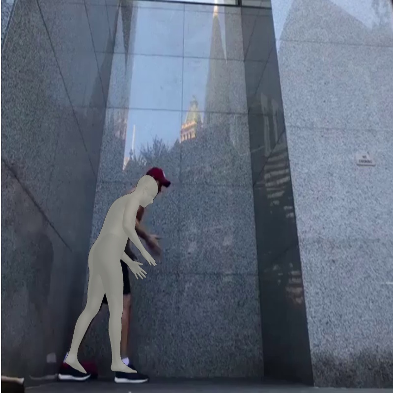
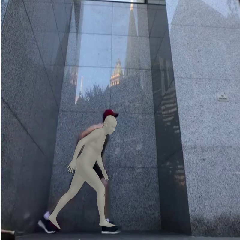
In addition to quantitative comparisons, we present 1) visual comparisons with the VIBE (Kocabas et al., 2020) and SPIN (Kolotouros et al., 2019a) methods, 2) visual results of occlusion handling, and 3) visual results of different viewpoints.
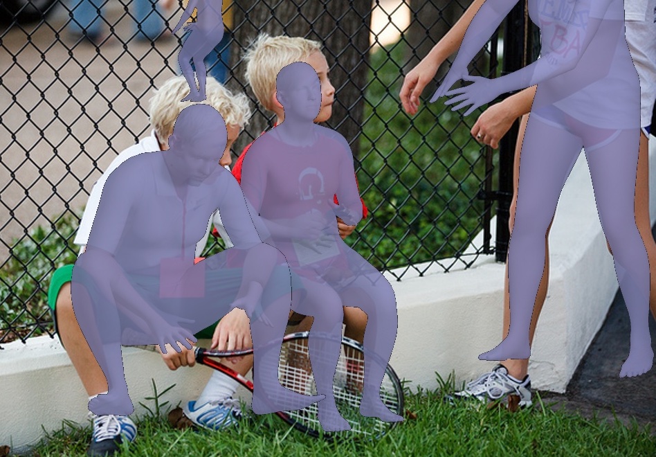
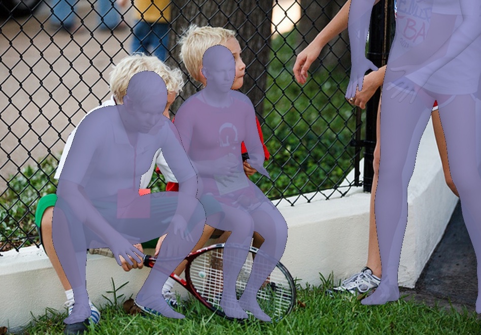
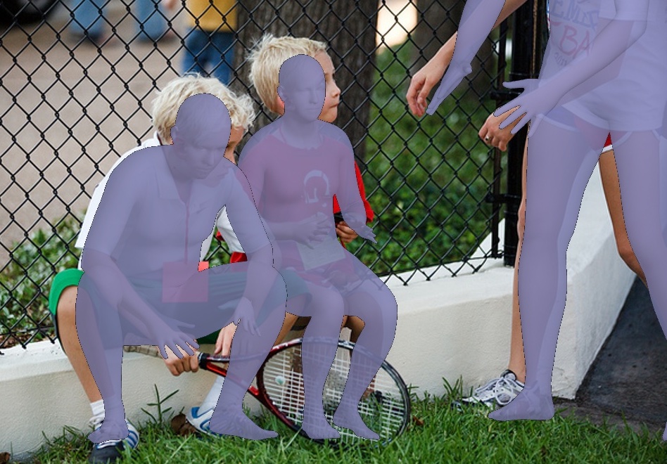
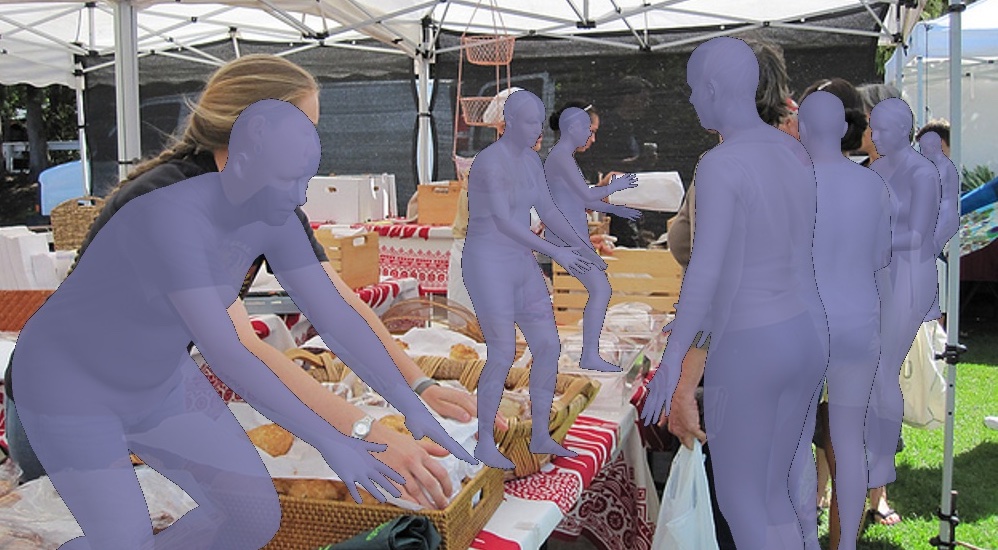
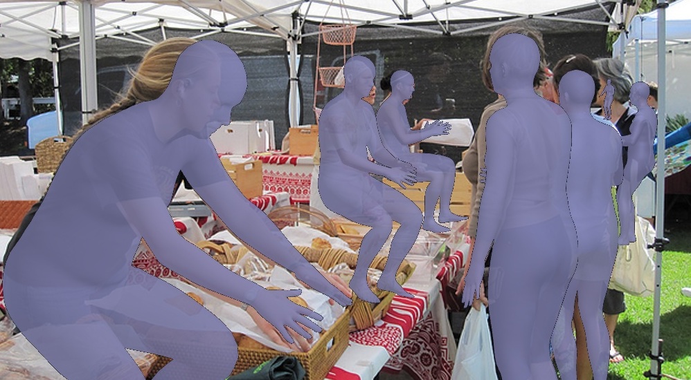
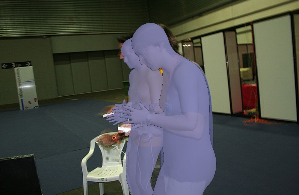
Visual comparisons with the VIBE and SPIN methods. Figure 6 shows two visual comparisons with the VIBE (Kocabas et al., 2020) and SPIN (Kolotouros et al., 2019a). We observe that our model recovers bodies that well cover humans and estimates more accurate poses for limbs in particular.
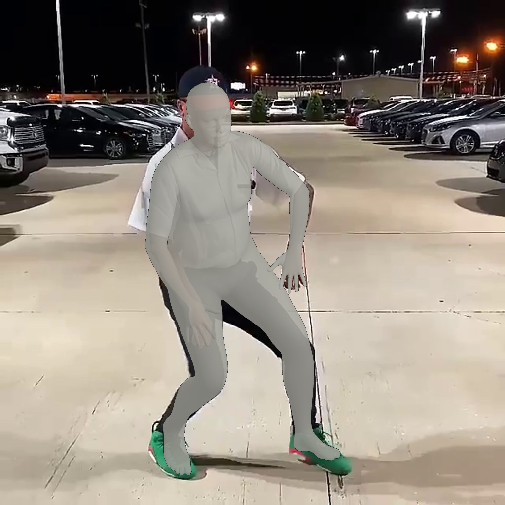
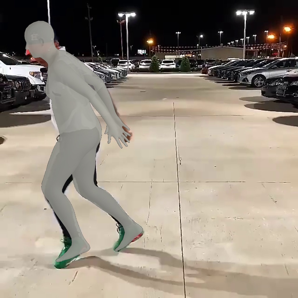
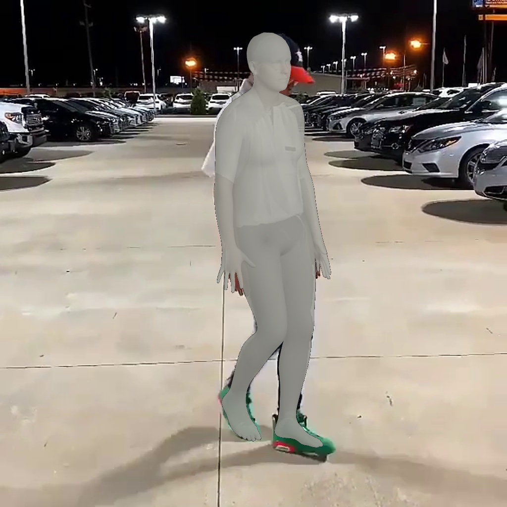
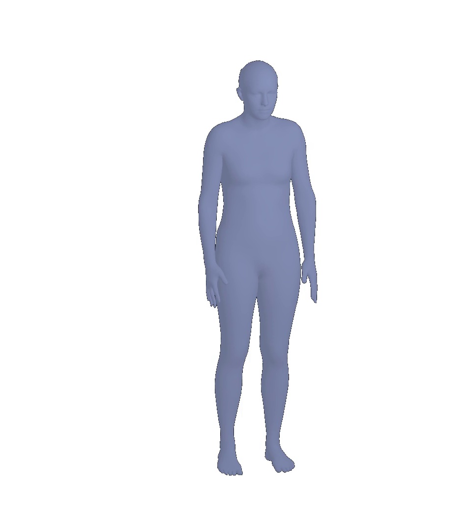
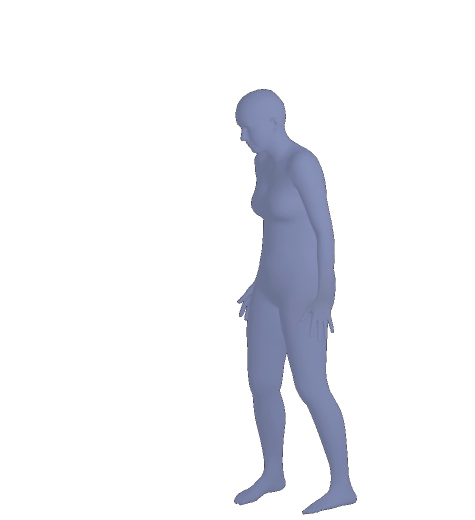
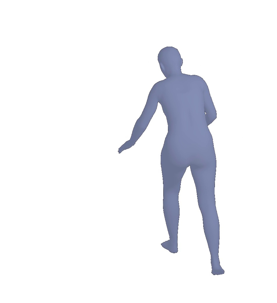
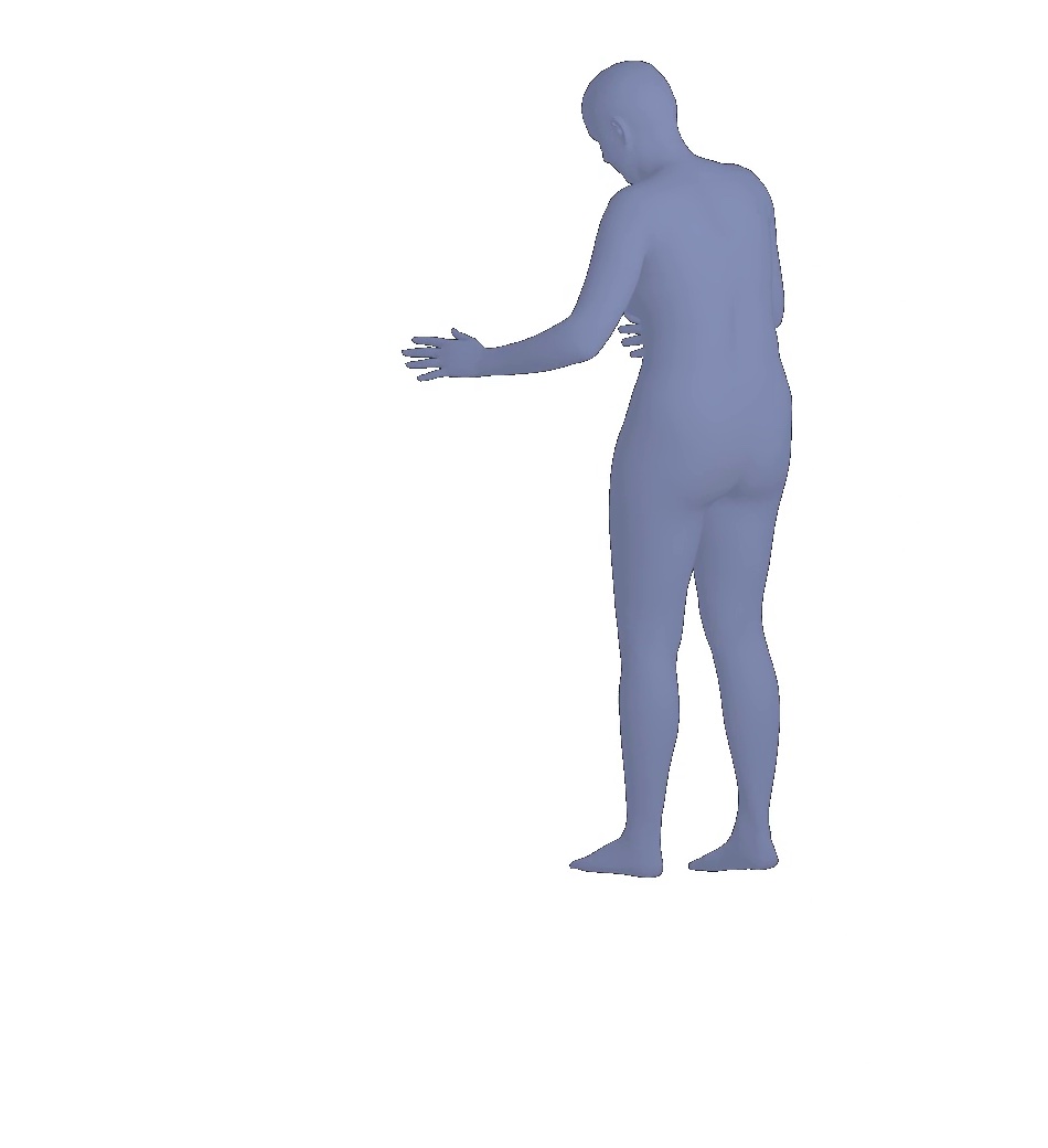
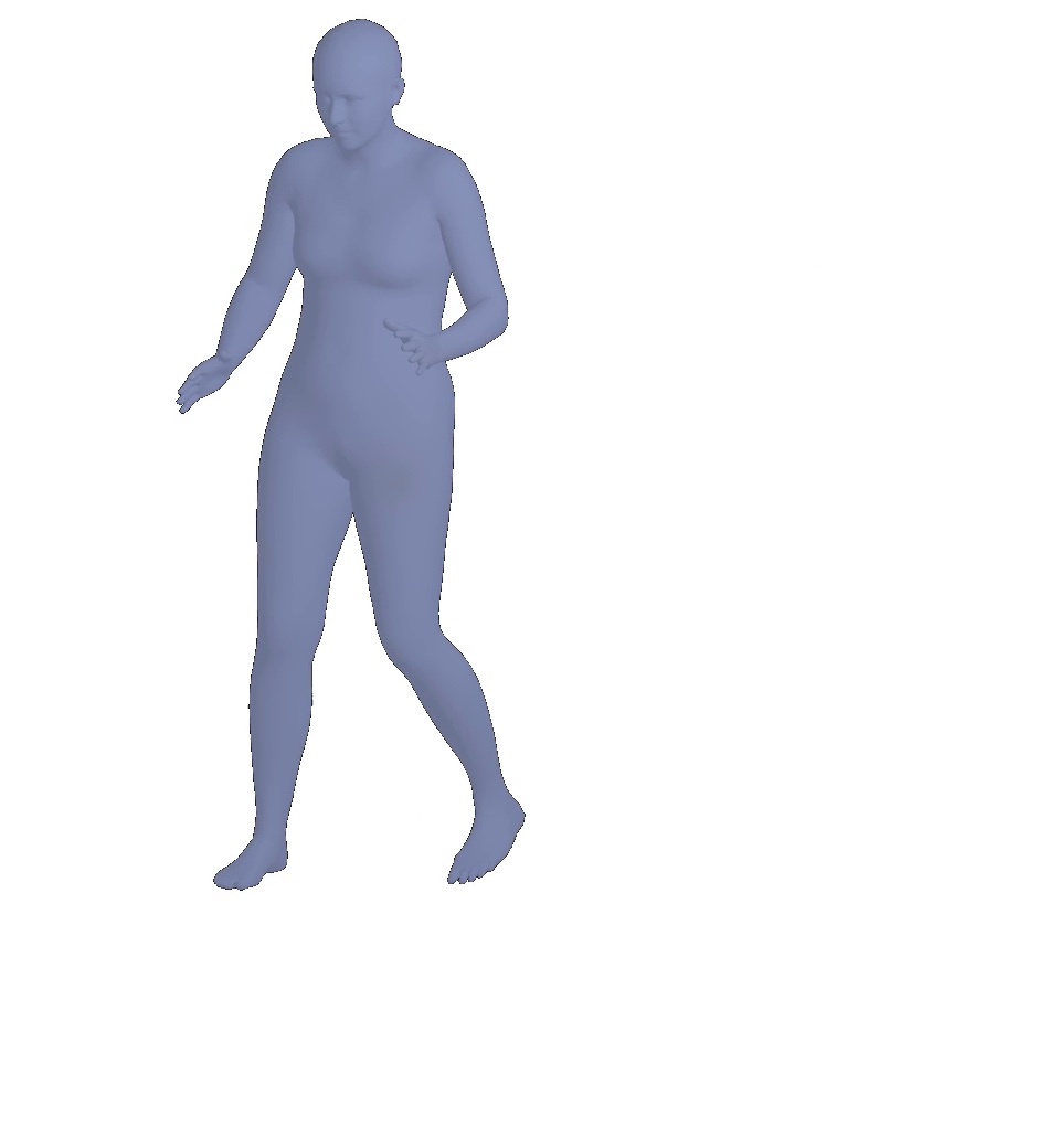
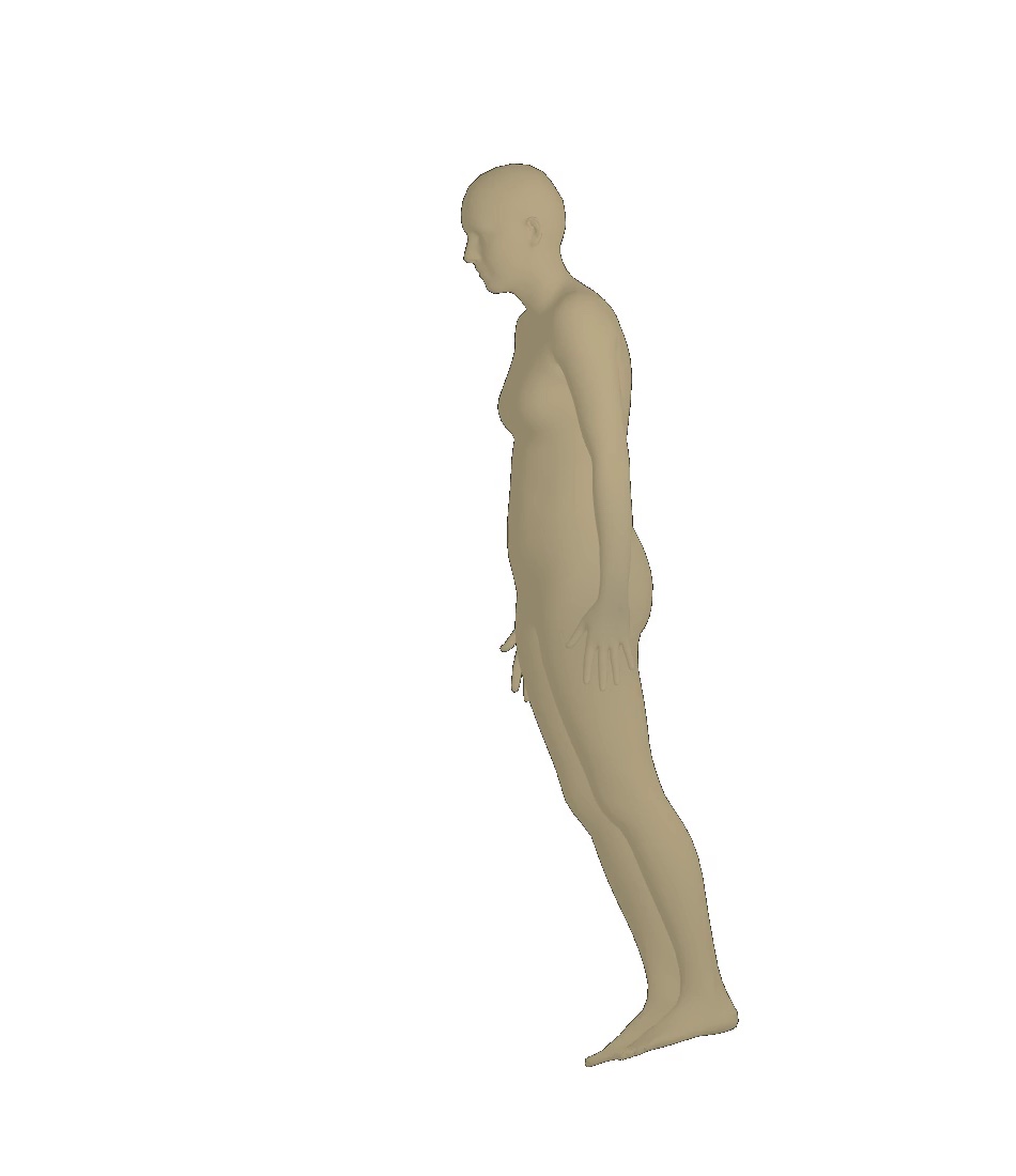
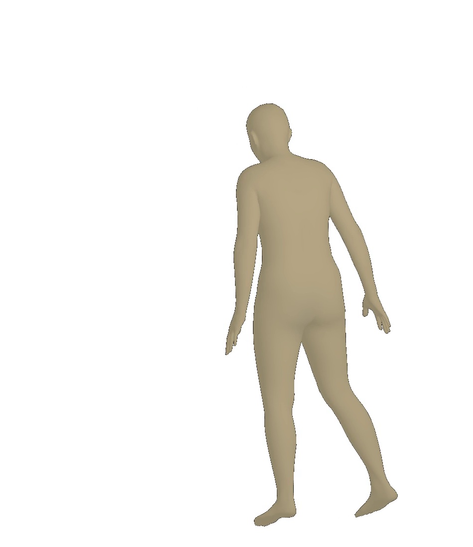
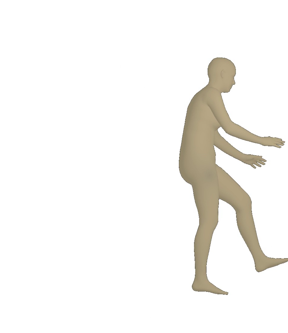
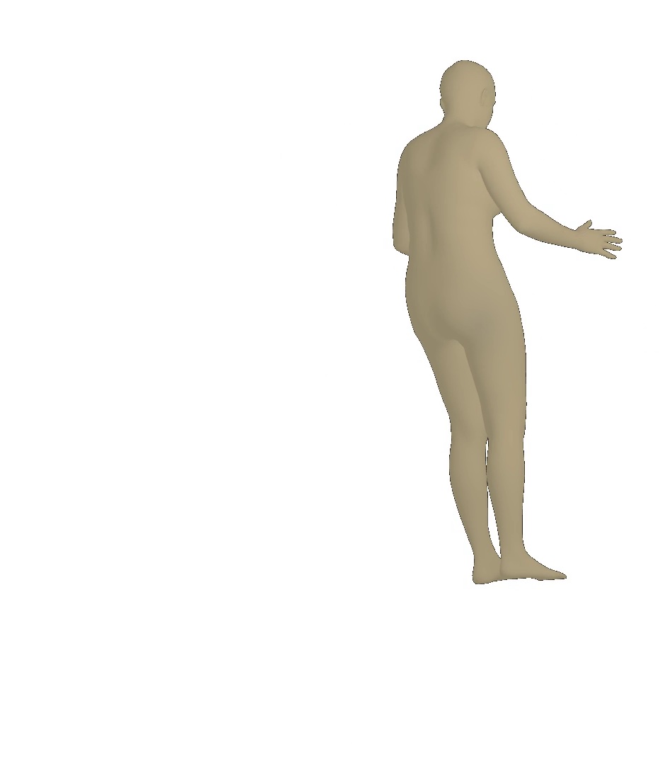
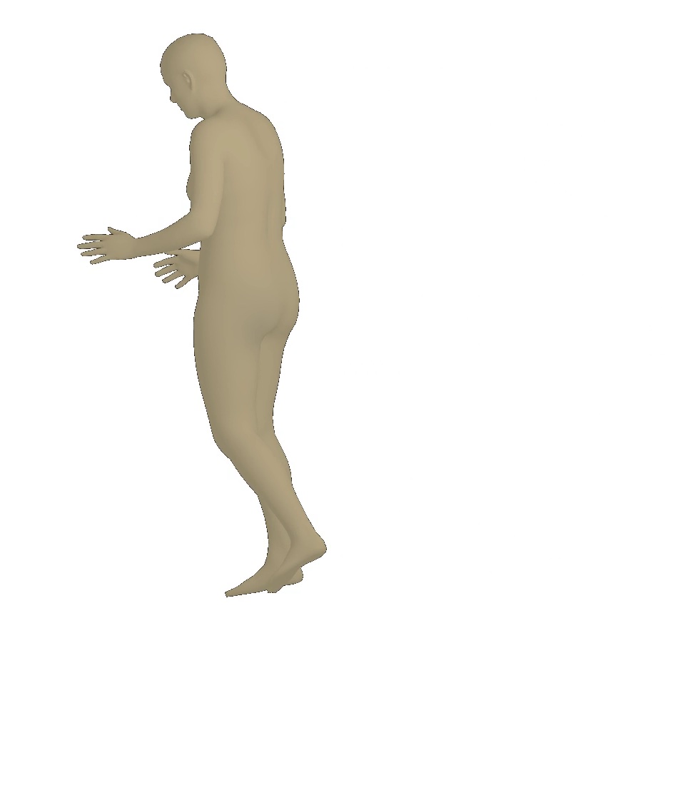
Visual results of different viewpoints. We visualize human bodies recovered by our SPS-Net from different viewpoints in Figure 8. Our results show that our method estimates accurate rotation parameters.
4.4 Ablation study
Loss functions. To analyze the effectiveness of each loss function, we conduct an ablation study by removing one loss function at a time. Specifically, we analyze how much performance gain each loss function contributes. Table 2 shows the results on the 3DPW (von Marcard et al., 2018) test set.
Without the camera parameter consistency loss , there is no explicit constraint imposed on the prediction of camera parameters, leading to performance drops of in PA-MPJPE and in PVE. When removing the mask loss , our model does not have any constraints to regularize the 3D mesh. Performance drops of in PA-MPJPE and in PVE occur. Without the self-supervised parameter regression loss , our model does not learn to produce plausible predictions when the occlusion or out-of-view issues occur, resulting in performance drops of in PA-MPJPE and in PVE. When removing the adversarial loss , our model does not learn to render 3D meshes that have realistic motions. Performance drops on all three evaluation metrics occur, which also concur with the findings in the HMR (Kanazawa et al., 2018) and VIBE (Kocabas et al., 2020).
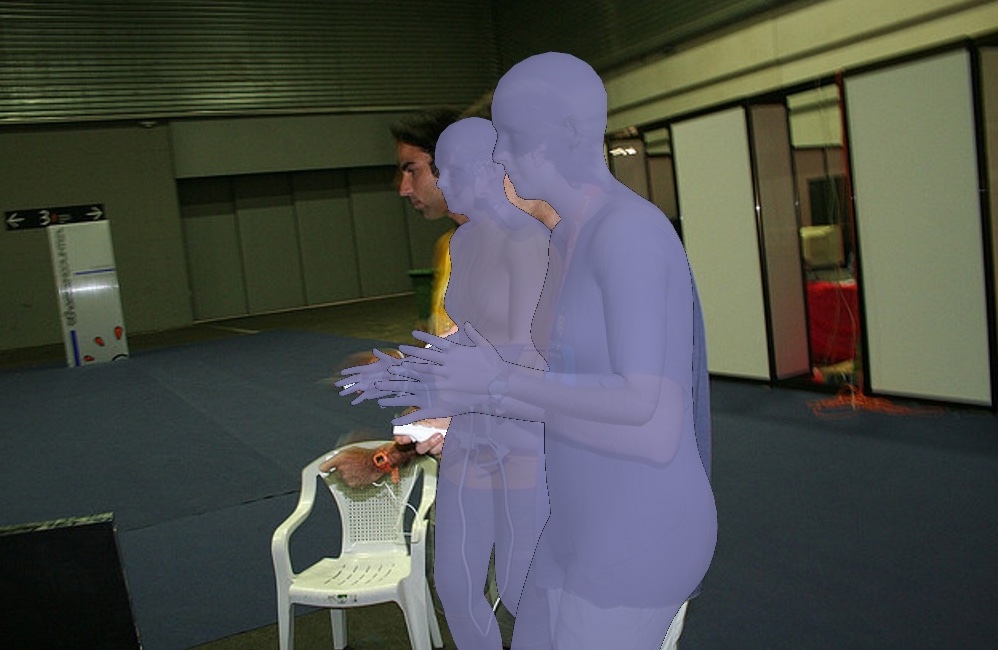
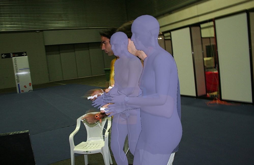
Figure 9 presents two visual comparisons with the variant methods of our SPS-Net (i.e., Ours w/o and Ours w/o ). Our visual results show that both the camera parameter consistency loss and the mask loss allow our model to predict more accurate pose and shape estimates.
The ablation study on loss functions shows that all four losses are crucial to the SPS-Net.
| Method | PA-MPJPE | MPJPE | PVE |
|---|---|---|---|
| Ours | 50.4 | 85.8 | 100.6 |
| Ours w/o | 52.1 | 88.2 | 104.1 |
| Ours w/o | 56.3 | 90.0 | 107.6 |
| Ours w/o | 55.8 | 89.4 | 105.2 |
| Ours w/o | 56.2 | 93.4 | 112.5 |
| Method | PA-MPJPE | MPJPE | PVE | ||
|---|---|---|---|---|---|
| Ours | 51.43M | 50.4 | 85.8 | 100.6 | 22.1 |
| Ours w/o Forecasting | 47.23M | 54.2 | 91.9 | 104.3 | 23.3 |
| Ours w/o Self-Attention | 34.64M | 57.6 | 96.6 | 104.7 | 22.9 |
Self-attention and forecasting modules. We conduct an ablation study to analyze the contribution of the self-attention module and the forecasting module in the SPS-Net. Specifically, we show the contribution of each component by disabling (removing) one at a time. Table 3 shows the results on the 3DPW (von Marcard et al., 2018) test set. Without either the forecasting module or the self-attention module , the degraded method suffers from significant performance loss in all metrics. When both modules are jointly utilized, our model achieves the best results, demonstrating the complementary importance of these two components.
| Method | PA-MPJPE | MPJPE | PVE | |
|---|---|---|---|---|
| Ours (Self-Attention) | 51.43M | 50.4 | 85.8 | 100.6 |
| Ours (GRU) | 50.88M | 52.8 | 87.7 | 103.2 |
Self-attention module vs. GRU. To analyze the effectiveness of employing different temporal modules, we conduct an ablation study by swapping the self-attention module in the SPS-Net with a two-layer GRU module as in the VIBE (Kocabas et al., 2020) model, i.e., comparing the performance between the “Ours (Self-Attention)” method and the “Ours (GRU)” approach. Table 4 presents the results on the 3DPW (von Marcard et al., 2018) test set. We observe that employing the self-attention module results in performance improvement over adopting the GRU on all three evaluation metrics.
| Input sequence length | PA-MPJPE | MPJPE | PVE |
|---|---|---|---|
| 8 | 55.3 | 92.4 | 110.8 |
| 16 | 53.1 | 87.6 | 105.5 |
| 32 | 50.4 | 85.8 | 100.6 |
| 48 | 50.2 | 85.1 | 100.2 |
| Method | Platform | Training | Inference |
|---|---|---|---|
| Yang et al. (Yang et al., 2018) | Titan X | - | 1.1 |
| Mehta et al. (Mehta et al., 2017b) | Titan X | - | 3.3 |
| RepNet (Wandt and Rosenhahn, 2019) | Titan X | - | 10 |
| CMR (Kolotouros et al., 2019b) | RTX 2080Ti | - | 3.3 |
| STRAPS (Sengupta et al., 2020) | RTX 2080Ti | 120 | 0.25 |
| NBF (Omran et al., 2018) | V100 | 18 | - |
| ExPose (Choutas et al., 2020) | Quadro P5000 | - | 0.16 |
| HUND (Zanfir et al., 2020) | P100 | 72 | 0.055 |
| HMR (Kanazawa et al., 2018) | Titan 1080Ti | 120 | 0.04 |
| SPIN (Kolotouros et al., 2019a) | - | - | 3 |
| Temporal 3D Kinetics (Arnab et al., 2019) | - | - | 2 |
| VIBE (Kocabas et al., 2020) | RTX 2080Ti | 1 | 0.07 |
| Ours | V100 | 12 | 0.09 |
Input sequence length. We conduct an ablation study to analyze the effect of the input sequence length. Table 5 presents the results on the 3DPW (von Marcard et al., 2018) dataset. Our results show that the performance on all three metrics improves as the input sequence length increases. When the input sequence length increases from (the default setting in our experiments) to , our results can be further improved. However, due to GPU memory constraints, we are not able to experiment with longer input sequence lengths.
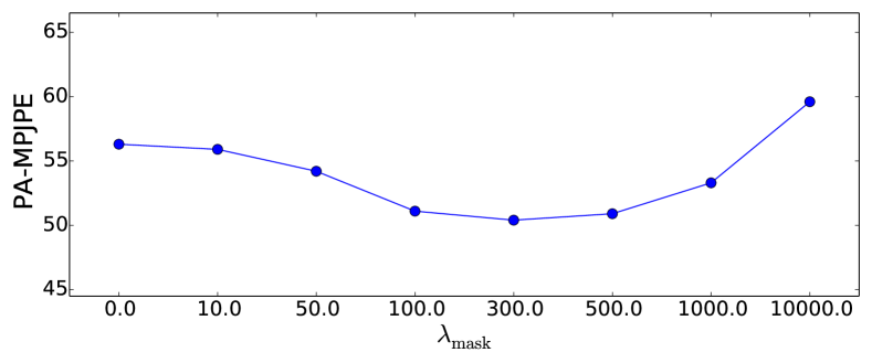
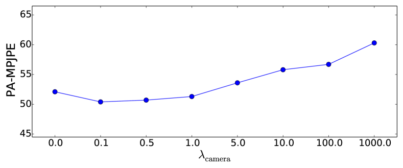
Sensitivity analysis. To analyze the sensitivity of the SPS-Net with respect to the hyperparameters, we perform a sensitivity analysis on the hyperparameters and . We report the PA-MPJPE results on the 3DPW (von Marcard et al., 2018) test set. Figure 10 presents the experimental results.
We observe that when the hyperparameter is set to (i.e., the corresponding loss function is removed), our SPS-Net suffers from performance drops. When the hyperparameters are set within a suitable range (i.e., around for and around for ), the performance of our SPS-Net is improved, demonstrating the effectiveness of the corresponding loss function. When the hyperparameters are set to large values (e.g., for and for ), our model training will be dominated by optimizing the corresponding loss, leading to performance drops.
The sensitivity analysis of hyperparameters shows that when each hyperparameter is set within a suitable range, the performance of our method is improved and remains stable.
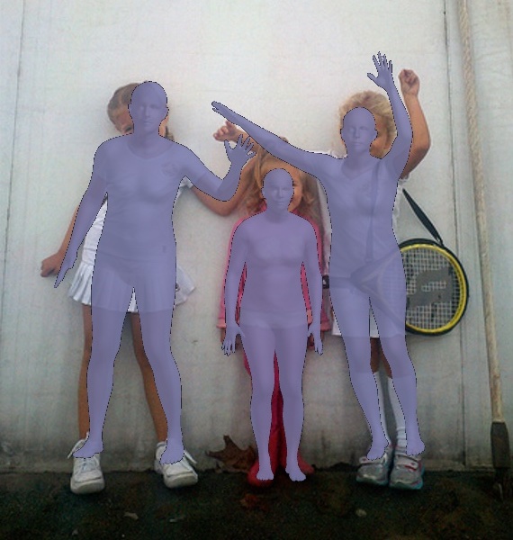
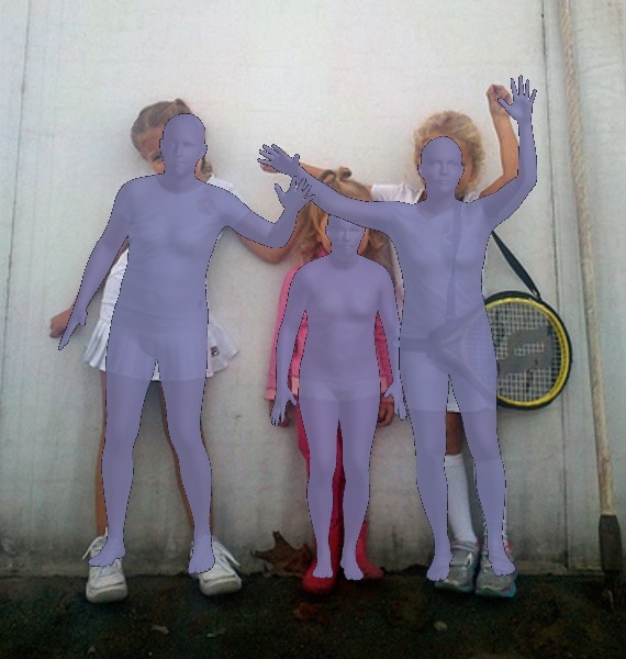
4.6 Failure modes
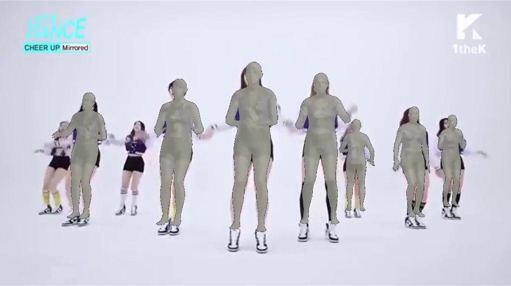
We present the failure cases of our method in Figure 11. As our SPS-Net assumes that the input video frames contain a single person, if missing detection happens, our method will not be able to perform human pose and shape estimation.

Ours w/o Self-Attention
Ours w/o Forecasting
Ours
5 Conclusions
We propose the SPS-Net for estimating 3D human pose and shape from videos. The main contributions of this work lie in the design of the self-attention module that captures short-range and long-range dependencies across video frames and the forecasting module that allows our model to exploit visual cues from human motion for producing temporally coherent predictions. To address the absence of ground-truth camera parameter annotations, we propose a camera parameter consistency loss that not only regularizes the learning of camera parameter prediction but also provides additional supervisory signals to facilitate model training. We develop a self-supervised learning scheme that explicitly models the occlusion and out-of-view scenarios by masking out some regions in the video frames. By leveraging the predictions of the original video frames to supervise those of the synthesized occluded or partially visible data, our model learns to predict plausible estimations. Extensive experimental results on three challenging datasets show that our SPS-Net performs favorably against the state-of-the-art 3D human pose and shape estimation methods.
References
- Andriluka et al. (2018) Andriluka, M., Iqbal, U., Insafutdinov, E., Pishchulin, L., Milan, A., Gall, J., Schiele, B., 2018. Posetrack: A benchmark for human pose estimation and tracking, in: CVPR.
- Arnab et al. (2019) Arnab, A., Doersch, C., Zisserman, A., 2019. Exploiting temporal context for 3d human pose estimation in the wild, in: CVPR.
- Bewley et al. (2016) Bewley, A., Ge, Z., Ott, L., Ramos, F., Upcroft, B., 2016. Simple online and realtime tracking, in: ICIP.
- Bochkovskiy et al. (2020) Bochkovskiy, A., Wang, C.Y., Liao, H.Y.M., 2020. Yolov4: Optimal speed and accuracy of object detection. arXiv .
- Bogo et al. (2016) Bogo, F., Kanazawa, A., Lassner, C., Gehler, P., Romero, J., Black, M.J., 2016. Keep it smpl: Automatic estimation of 3d human pose and shape from a single image, in: ECCV.
- Bolya et al. (2019) Bolya, D., Zhou, C., Xiao, F., Lee, Y.J., 2019. Yolact: real-time instance segmentation, in: ICCV.
- Butepage et al. (2017) Butepage, J., Black, M.J., Kragic, D., Kjellstrom, H., 2017. Deep representation learning for human motion prediction and classification, in: CVPR.
- Cao et al. (2019) Cao, Z., Martinez, G.H., Simon, T., Wei, S.E., Sheikh, Y.A., 2019. Openpose: Realtime multi-person 2d pose estimation using part affinity fields. TPAMI .
- Chen et al. (2019a) Chen, C.H., Tyagi, A., Agrawal, A., Drover, D., Stojanov, S., Rehg, J.M., 2019a. Unsupervised 3d pose estimation with geometric self-supervision, in: CVPR.
- Chen et al. (2019b) Chen, Y.C., Lin, Y.Y., Yang, M.H., Huang, J.B., 2019b. Crdoco: Pixel-level domain transfer with cross-domain consistency, in: CVPR.
- Chen et al. (2020) Chen, Y.C., Lin, Y.Y., Yang, M.H., Huang, J.B., 2020. Show, match and segment: Joint weakly supervised learning of semantic matching and object co-segmentation. TPAMI .
- Cheng et al. (2020) Cheng, Y., Yang, B., Wang, B., Tan, R.T., 2020. 3d human pose estimation using spatio-temporal networks with explicit occlusion training, in: AAAI.
- Choutas et al. (2020) Choutas, V., Pavlakos, G., Bolkart, T., 2020. Monocular expressive body regression through body-driven attention, in: ECCV.
- Denton and Birodkar (2017) Denton, E., Birodkar, V., 2017. Unsupervised learning of disentangled representations from video, in: NeurIPS.
- Doersch and Zisserman (2019) Doersch, C., Zisserman, A., 2019. Sim2real transfer learning for 3d human pose estimation: motion to the rescue, in: NeurIPS.
- Finn et al. (2016) Finn, C., Goodfellow, I., Levine, S., 2016. Unsupervised learning for physical interaction through video prediction, in: NeurIPS.
- Fragkiadaki et al. (2015) Fragkiadaki, K., Levine, S., Felsen, P., Malik, J., 2015. Recurrent network models for human dynamics, in: ICCV.
- Girdhar et al. (2018) Girdhar, R., Gkioxari, G., Torresani, L., Paluri, M., Tran, D., 2018. Detect-and-track: Efficient pose estimation in videos, in: CVPR.
- Gordon et al. (2019) Gordon, A., Li, H., Jonschkowski, R., Angelova, A., 2019. Depth from videos in the wild: Unsupervised monocular depth learning from unknown cameras, in: ICCV.
- He et al. (2016) He, K., Zhang, X., Ren, S., Sun, J., 2016. Deep residual learning for image recognition, in: CVPR.
- Huang et al. (2018) Huang, X., Liu, M.Y., Belongie, S., Kautz, J., 2018. Multimodal unsupervised image-to-image translation, in: ECCV.
- Ionescu et al. (2013) Ionescu, C., Papava, D., Olaru, V., Sminchisescu, C., 2013. Human3. 6m: Large scale datasets and predictive methods for 3d human sensing in natural environments. TPAMI .
- Jain et al. (2016) Jain, A., Zamir, A.R., Savarese, S., Saxena, A., 2016. Structural-rnn: Deep learning on spatio-temporal graphs, in: CVPR.
- Kanazawa et al. (2018) Kanazawa, A., Black, M.J., Jacobs, D.W., Malik, J., 2018. End-to-end recovery of human shape and pose, in: CVPR.
- Kanazawa et al. (2019) Kanazawa, A., Zhang, J.Y., Felsen, P., Malik, J., 2019. Learning 3d human dynamics from video, in: CVPR.
- Kay et al. (2017) Kay, W., Carreira, J., Simonyan, K., Zhang, B., Hillier, C., Vijayanarasimhan, S., Viola, F., Green, T., Back, T., Natsev, P., Suleyman, M., Zisserman, A., 2017. The kinetics human action video dataset. arXiv .
- Kingma and Ba (2014) Kingma, D.P., Ba, J., 2014. Adam: A method for stochastic optimization, in: ICLR.
- Kocabas et al. (2020) Kocabas, M., Athanasiou, N., Black, M.J., 2020. Vibe: Video inference for human body pose and shape estimation, in: CVPR.
- Kocabas et al. (2019) Kocabas, M., Karagoz, S., Akbas, E., 2019. Self-supervised learning of 3d human pose using multi-view geometry, in: CVPR.
- Kolotouros et al. (2019a) Kolotouros, N., Pavlakos, G., Black, M.J., Daniilidis, K., 2019a. Learning to reconstruct 3d human pose and shape via model-fitting in the loop, in: ICCV.
- Kolotouros et al. (2019b) Kolotouros, N., Pavlakos, G., Daniilidis, K., 2019b. Convolutional mesh regression for single-image human shape reconstruction, in: CVPR.
- Lassner et al. (2017) Lassner, C., Romero, J., Kiefel, M., Bogo, F., Black, M.J., Gehler, P.V., 2017. Unite the people: Closing the loop between 3d and 2d human representations, in: CVPR.
- Lee et al. (2018a) Lee, H.Y., Tseng, H.Y., Huang, J.B., Singh, M., Yang, M.H., 2018a. Diverse image-to-image translation via disentangled representations, in: ECCV.
- Lee et al. (2018b) Lee, K., Lee, I., Lee, S., 2018b. Propagating lstm: 3d pose estimation based on joint interdependency, in: ECCV.
- Li et al. (2019) Li, J., Wang, C., Zhu, H., Mao, Y., Fang, H.S., Lu, C., 2019. Crowdpose: Efficient crowded scenes pose estimation and a new benchmark, in: CVPR.
- Li et al. (2018) Li, Z., Zhou, Y., Xiao, S., He, C., Huang, Z., Li, H., 2018. Auto-conditioned recurrent networks for extended complex human motion synthesis, in: ICLR.
- Liu et al. (2019) Liu, L., Xu, W., Zollhoefer, M., Kim, H., Bernard, F., Habermann, M., Wang, W., Theobalt, C., 2019. Neural rendering and reenactment of human actor videos. ACM TOG .
- Loper et al. (2015) Loper, M., Mahmood, N., Romero, J., Pons-Moll, G., Black, M.J., 2015. Smpl: A skinned multi-person linear model. ACM TOG .
- Mahmood et al. (2019) Mahmood, N., Ghorbani, N., Troje, N.F., Pons-Moll, G., Black, M.J., 2019. Amass: Archive of motion capture as surface shapes, in: ICCV.
- von Marcard et al. (2018) von Marcard, T., Henschel, R., Black, M.J., Rosenhahn, B., Pons-Moll, G., 2018. Recovering accurate 3d human pose in the wild using imus and a moving camera, in: ECCV.
- Mehta et al. (2017a) Mehta, D., Rhodin, H., Casas, D., Fua, P., Sotnychenko, O., Xu, W., Theobalt, C., 2017a. Monocular 3d human pose estimation in the wild using improved cnn supervision, in: 3DV.
- Mehta et al. (2017b) Mehta, D., Sridhar, S., Sotnychenko, O., Rhodin, H., Shafiei, M., Seidel, H.P., Xu, W., Casas, D., Theobalt, C., 2017b. Vnect: Real-time 3d human pose estimation with a single rgb camera. ACM TOG .
- Meister et al. (2018) Meister, S., Hur, J., Roth, S., 2018. Unflow: Unsupervised learning of optical flow with a bidirectional census loss, in: AAAI.
- Omran et al. (2018) Omran, M., Lassner, C., Pons-Moll, G., Gehler, P., Schiele, B., 2018. Neural body fitting: Unifying deep learning and model based human pose and shape estimation, in: 3DV.
- Parmar et al. (2018) Parmar, N., Vaswani, A., Uszkoreit, J., Kaiser, Ł., Shazeer, N., Ku, A., Tran, D., 2018. Image transformer, in: ICML.
- Pascanu et al. (2013) Pascanu, R., Mikolov, T., Bengio, Y., 2013. On the difficulty of training recurrent neural networks, in: ICML.
- Paszke et al. (2019) Paszke, A., Gross, S., Massa, F., Lerer, A., Bradbury, J., Chanan, G., Killeen, T., Lin, Z., Gimelshein, N., Antiga, L., Desmaison, A., Köpf, A., Yang, E., DeVito, Z., Raison, M., Tejani, A., Chilamkurthy, S., Steiner, B., Fang, L., Bai, J., Chintala, S., 2019. Pytorch: An imperative style, high-performance deep learning library, in: NeurIPS.
- Pishchulin et al. (2016) Pishchulin, L., Insafutdinov, E., Tang, S., Andres, B., Andriluka, M., Gehler, P.V., Schiele, B., 2016. Deepcut: Joint subset partition and labeling for multi person pose estimation, in: CVPR.
- Rayat Imtiaz Hossain and Little (2018) Rayat Imtiaz Hossain, M., Little, J.J., 2018. Exploiting temporal information for 3d human pose estimation, in: ECCV.
- Sengupta et al. (2020) Sengupta, A., Budvytis, I., Cipolla, R., 2020. Synthetic training for accurate 3d human pose and shape estimation in the wild. arXiv .
- Sun et al. (2019) Sun, Y., Ye, Y., Liu, W., Gao, W., Fu, Y., Mei, T., 2019. Human mesh recovery from monocular images via a skeleton-disentangled representation, in: ICCV.
- Vaswani et al. (2017) Vaswani, A., Shazeer, N., Parmar, N., Uszkoreit, J., Jones, L., Gomez, A.N., Kaiser, Ł., Polosukhin, I., 2017. Attention is all you need, in: NeurIPS.
- Villegas et al. (2018) Villegas, R., Yang, J., Ceylan, D., Lee, H., 2018. Neural kinematic networks for unsupervised motion retargetting, in: CVPR.
- Walker et al. (2016) Walker, J., Doersch, C., Gupta, A., Hebert, M., 2016. An uncertain future: Forecasting from static images using variational autoencoders, in: ECCV.
- Walker et al. (2017) Walker, J., Marino, K., Gupta, A., Hebert, M., 2017. The pose knows: Video forecasting by generating pose futures, in: ICCV.
- Wandt and Rosenhahn (2019) Wandt, B., Rosenhahn, B., 2019. Repnet: Weakly supervised training of an adversarial reprojection network for 3d human pose estimation, in: CVPR.
- Xu et al. (2019) Xu, W., Chatterjee, A., Zollhoefer, M., Rhodin, H., Fua, P., Seidel, H.P., Theobalt, C., 2019. Mo 2 cap 2: Real-time mobile 3d motion capture with a cap-mounted fisheye camera. TVCG .
- Yang et al. (2018) Yang, W., Ouyang, W., Wang, X., Ren, J., Li, H., Wang, X., 2018. 3d human pose estimation in the wild by adversarial learning, in: CVPR.
- Zanfir et al. (2020) Zanfir, A., Bazavan, E.G., Zanfir, M., Freeman, W.T., Sukthankar, R., Sminchisescu, C., 2020. Neural descent for visual 3d human pose and shape. arXiv .
- Zhang et al. (2019a) Zhang, H., Goodfellow, I., Metaxas, D., Odena, A., 2019a. Self-attention generative adversarial networks, in: ICML.
- Zhang et al. (2019b) Zhang, J.Y., Felsen, P., Kanazawa, A., Malik, J., 2019b. Predicting 3d human dynamics from video, in: ICCV.
- Zhang et al. (2013) Zhang, W., Zhu, M., Derpanis, K.G., 2013. From actemes to action: A strongly-supervised representation for detailed action understanding, in: ICCV.
- Zhou et al. (2017) Zhou, T., Brown, M., Snavely, N., Lowe, D.G., 2017. Unsupervised learning of depth and ego-motion from video, in: CVPR.
- Zhou et al. (2015) Zhou, T., Jae Lee, Y., Yu, S.X., Efros, A.A., 2015. Flowweb: Joint image set alignment by weaving consistent, pixel-wise correspondences, in: CVPR.
- Zhu et al. (2017) Zhu, J.Y., Park, T., Isola, P., Efros, A.A., 2017. Unpaired image-to-image translation using cycle-consistent adversarial networks, in: ICCV.
- Zou et al. (2018) Zou, Y., Luo, Z., Huang, J.B., 2018. Df-net: Unsupervised joint learning of depth and flow using cross-task consistency, in: ECCV.