∎

¹¹institutetext: Tran Ngoc Thang ²²institutetext: School of Applied Mathematics and Informatics, Hanoi University of Science and Technology,
1st Dai Co Viet, Hai Ba Trung, Hanoi, Viet Nam
²²email: [email protected] ³³institutetext: Trinh Ngoc Hai ( ✉ ) ⁴⁴institutetext: School of Applied Mathematics and Informatics, Hanoi University of Science and Technology,
1st Dai Co Viet, Hai Ba Trung, Hanoi, Viet Nam
⁴⁴email: [email protected]

Self-adaptive algorithms for quasiconvex programming and applications to machine learning

Tran Ngoc Thang Trinh Ngoc Hai

Abstract

For solving a broad class of nonconvex programming problems on an unbounded constraint set, we provide a self-adaptive step-size strategy that does not include line-search techniques and establishes the convergence of a generic approach under mild assumptions. Specifically, the objective function may not satisfy the convexity condition. Unlike descent line-search algorithms, it does not need a known Lipschitz constant to figure out how big the first step should be. The crucial feature of this process is the steady reduction of the step size until a certain condition is fulfilled. In particular, it can provide a new gradient projection approach to optimization problems with an unbounded constrained set. The correctness of the proposed method is verified by preliminary results from some computational examples. To demonstrate the effectiveness of the proposed technique for large-scale problems, we apply it to some experiments on machine learning, such as supervised feature selection, multi-variable logistic regressions and neural networks for classification.

Keywords:

nonconvex programming gradient descent algorithms quasiconvex functions pseudoconvex functions self-adaptive step-sizes

MSC:

90C25 90C26 68Q32 93E35

1 Introduction

Gradient descent methods are a common tool for a wide range of programming problems, from convex to nonconvex, and have numerous practical applications (see Boyd , Cevher , Lan and references therein). At each iteration, gradient descent algorithms provide an iterative series of solutions based on gradient directions and step sizes. For a long time, researchers have focused on finding the direction to improve the convergence rate of techniques, while the step-size was determined using one of the few well-known approaches (see Boyd , Nesterov ).

Recently, new major areas of machine learning applications with high dimensionality and nonconvex objective functions have required the development of novel step-size choosing procedures to reduce the method’s overall computing cost (see Cevher , Lan ). The exact or approximate one-dimensional minimization line-search incurs significant computational costs per iteration, particularly when calculating the function value is nearly identical to calculating its derivative and requires the solution of complex auxiliary problems (see Boyd ). To avoid the line-search, the step-size value may be calculated using prior information such as Lipschitz constants for the gradient. However, this requires using just part of their inexact estimations, which leads to slowdown convergence. This is also true for the well-known divergent series rule (see Kiwiel , Nesterov ).

Although Kiwiel developed the gradient approach for quasiconvex programming in 2001 Kiwiel , it results in slow convergence due to the use of diminishing step-size. Following that, there are some improvements to the gradient method, such as the work of Yu et al. (Yu , 2019), Hu et al. (Hu , 2020), which use a constant step-size but the objective function must fulfil the Hölder condition. The other method is the neurodynamic approach, which uses recurrent neural network models to solve pseudoconvex programming problems with unbounded constraint sets (see Bian (Bian et al, 2018), Liu (Liu et al., 2022)). Its step-size selection is fixed and not adaptive.

The adaptive step-size procedure was proposed in Konnov (Konnov, 2018) and Ferreira (Ferreira et. al., 2020) . The method given in Konnov , whereby a step-size algorithm for the conditional gradient method is proposed, is effective for solving pseudoconvex programming problems with the boundedness of the feasible set. It has been expanded in Ferreira to the particular case of an unbounded feasible set, which cannot be applied to the unconstrained case. In this research, we propose a novel and line-search-free adaptive step-size algorithm for a broad class of programming problems where the objective function is nonconvex and smooth, the constraint set is unbounded, closed and convex. A crucial component of this procedure is gradually decreasing the step size until a predetermined condition is fulfilled. Although the Lipschitz continuity of the gradient of the objective function is required for convergence, the approach does not make use of predetermined constants. The proposed change has been shown to be effective in preliminary computational tests. We perform various machine learning experiments, including multi-variable logistic regressions and neural networks for classification, to show that the proposed method performs well on large-scale tasks.

The rest of this paper is structured as follows: Section 2 provides preliminary information and details the problem formulation. Section 3 summarizes the primary results, including the proposed algorithms. Section 4 depicts numerical experiments and analyzes their computational outcomes. Section 5 presents applications to certain machine learning problems. The final section draws some conclusions.

2 Preliminaries

In the whole paper, we assume that $C$ is a nonempty, closed and convex set in $\mathbb{R}^{m}$ , $f:\mathbb{R}^{m}\to\mathbb{R}$ is a differentiable function on an open set containing $C$ , the mapping $\nabla f$ is Lipschitz continuous. We consider the optimization problem:

\min\limits_{x\in C}f(x).

(OP(

f,C

))

Assume that the solution set of (OP( $f,C$ )) is not empty. First, we recall some definitions and basic results that will be used in the next section of the article. The interested reader is referred to BauschkeCombettes ; Rockafellar for bibliographical references.

For $x\in\mathbb{R}^{m}$ , denote by $P_{C}(x)$ the projection of $x$ onto $C$ , i.e.,

P_{C}(x):=\text{argmin}\{\|z-x\|:z\in C\}.

Proposition 1

BauschkeCombettes It holds that

(i)

$\|P_{C}(x)-P_{C}(y)\|\leq\|x-y\|$ for all $x,y\in\mathbb{R}^{m}$ ,
(ii)

$\left\langle y-P_{C}(x),x-P_{C}(x)\right\rangle\leq 0$ for all $x\in\mathbb{R}^{m}$ , $y\in C$ .

Definition 1

Mangasarian The function $f:\mathbb{R}^{m}\to\mathbb{R}$ is said to be

$\bullet$

convex on $C$ if for all $x,y\in C$ , $\lambda\in[0,1]$ , it holds that

$f(\lambda x+(1-\lambda)y)\leq\lambda f(x)+(1-\lambda)f(y).$
$\bullet$

pseudoconvex on $C$ if for all $x,y\in C$ , it holds that

$\langle\nabla f(x),y-x\rangle\geq 0\Rightarrow f(y)\geq f(x).$
$\bullet$

quasiconvex on $C$ if for all $x,y\in C$ , $\lambda\in[0;1]$ , it holds that

$f(\lambda x+(1-\lambda)y)\leq\max\left\{f(x);f(y)\right\}.$

Proposition 2

Dennis The differentiable function $f$ is quasiconvex on $C$ if and only if

f(y)\leq f(x)\Rightarrow\langle\nabla f(x),y-x\rangle\leq 0.

It is worth mentioning that ” $f$ is convex” $\Rightarrow$ ” $f$ is pseudoconvex” $\Rightarrow$ ” $f$ is quasiconvex”Mangasarian .

Proposition 3

Dennis Suppose that $\nabla f$ is $L$ -Lipschitz continuous on $C$ . For all $x,y\in C$ , it holds that

\left|f(y)-f(x)-\left<\nabla f(x),y-x\right>\right|\leq\dfrac{L}{2}\|y-x\|^{2}.

Lemma 1

Xu Let $\{a_{k}\}$ ; $\{b_{k}\}\subset(0;\infty)$ be sequences such that

a_{k+1}\leq a_{k}+b_{k}\ \forall k\geq 0;\quad\sum_{k=0}^{\infty}b_{k}<\infty.

Then, there exists the limit $\lim_{k\to\infty}a_{k}=c\in\mathbb{R}.$

3 Main results

Algorithm 1

(Algorithm GDA)
Step 0. Choose $x^{0}\in C$ , $\lambda_{0}\subset(0,+\infty)$ , $\sigma,\kappa\in(0,1)$ . Set $k=0$ .
Step 1. Given $x^{k}$ and $\lambda_{k}$ , compute $x^{k+1}$ and $\lambda_{k+1}$ as

	$\displaystyle x^{k+1}=P_{C}(x^{k}-\lambda_{k}\nabla f(x^{k})),$
	$\displaystyle\textbf{If }f(x^{k+1})\leq f(x^{k})-\sigma\left<\nabla f(x^{k}),x^{k}-x^{k+1}\right>\textbf{ then set }\lambda_{k+1}:=\lambda_{k}\textbf{ else set }\lambda_{k+1}:=\kappa\lambda_{k}.$

Step 2. Update $k:=k+1$ . If $x^{k+1}=x^{k}$ then STOP else go to Step 1.

Remark 1

If Algorithm 2 stops at step $k$ , then $x^{k}$ is a stationary point of the problem OP( $f,C$ ). Indeed, since $x^{k+1}=P_{C}\left(x^{k}-\lambda_{k}\nabla f(x^{k})\right)$ , applying Proposition 1-(ii), we have

\left<z-x^{k+1},x^{k}-\lambda_{k}\nabla f(x^{k})-x^{k+1}\right>\leq 0\ \forall z\in C.

(1)

If $x^{k+1}=x^{k}$ , we get

\left\langle\nabla f(x^{k}),z-x^{k}\right\rangle\geq 0\quad\forall z\in C,

(2)

which means $x^{k}$ is a stationary point of the problem. If, in addition, $f$ is pseudoconvex, from (2), it implies that $f(z)\geq f(x^{k})$ for all $z\in C$ , or $x^{k}$ is a solution of OP( $f,C$ ).

Now, suppose that the algorithms generates an infinite sequence. We will prove that this sequence converges to a solution of the problem OP( $f,C$ ).

Theorem 3.1

Assume that the sequence $\left\{x^{k}\right\}$ is generated by Algorithm 2. Then, the sequence $\left\{f(x^{k})\right\}$ is convergent and each limit point (if any) of the sequence $\left\{x^{k}\right\}$ is a stationary point of the problem. Moreover,

$\bullet$

if $f$ is quasiconvex on $C$ , then the sequence $\left\{x^{k}\right\}$ converges to a stationary point of the problem.
$\bullet$

if $f$ is pseudoconvex on $C$ , then the sequence $\left\{x^{k}\right\}$ converges to a solution of the problem.

Proof

Applying Proposition 3, we get

f(x^{k+1})\leq f(x^{k})+\left<\nabla f(x^{k}),x^{k+1}-x^{k}\right>+\frac{L}{2}\|x^{k+1}-x^{k}\|^{2}.

(3)

In (1), taking $z=x^{k}\in C$ , we arrive at

\left<\nabla f(x^{k}),x^{k+1}-x^{k}\right>\leq-\dfrac{1}{\lambda_{k}}\|x^{k+1}-x^{k}\|^{2}.

(4)

Combining (3) and (4), we obtain

f(x^{k+1})\leq f(x^{k})-\sigma\left<\nabla f(x^{k}),x^{k}-x^{k+1}\right>-\left(\frac{1-\sigma}{\lambda_{k}}-\frac{L}{2}\right)\|x^{k+1}-x^{k}\|^{2}.

(5)

We now claim that $\{\lambda_{k}\}$ is bounded away from zero, or in other words, the step size changes finite times. Indeed, suppose, by contrary, that $\lambda_{k}\to 0.$ From (5), there exists $k_{0}\in\mathbb{N}$ satisfying

f(x^{k+1})\leq f(x^{k})-\sigma\left<\nabla f(x^{k}),x^{k}-x^{k+1}\right>\ \forall k\geq k_{0}.

According to the construction of $\lambda_{k}$ , the last inequality implies that $\lambda_{k}=\lambda_{k_{0}}$ for all $k\geq k_{0}$ . This is a contradiction. And so, there exists $k_{1}\in\mathbb{N}$ such that for all $k\geq k_{1}$ , we have $\lambda_{k}=\lambda_{k_{1}}$ and

f(x^{k+1})\leq f(x^{k})-\sigma\left<\nabla f(x^{k}),x^{k}-x^{k+1}\right>.

(6)

Noting that $\left<\nabla f(x^{k}),x^{k}-x^{k+1}\right>\geq 0$ , we infer that the sequence $\{f(x^{k})\}$ is convergent and

\sum_{k=0}^{\infty}\left<\nabla f(x^{k}),x^{k}-x^{k+1}\right><\infty;\quad\sum_{k=0}^{\infty}\|x^{k+1}-x^{k}\|^{2}<\infty.

(7)

From (1), for all $z\in C$ , we have

	$\displaystyle\\|x^{k+1}-z\\|^{2}$	$\displaystyle=\\|x^{k}-z\\|^{2}-\\|x^{k+1}-x^{k}\\|^{2}+2\left\langle x^{k+1}-x^{k},x^{k+1}-z\right\rangle$
		$\displaystyle\leq\\|x^{k}-z\\|^{2}-\\|x^{k+1}-x^{k}\\|^{2}+2\lambda_{k}\left\langle\nabla f(x^{k}),z-x^{k+1}\right\rangle.$		(8)

Let $\bar{x}$ be a limit point of $\left\{x^{k}\right\}$ . There exists a subsequence $\left\{x^{k_{i}}\right\}\subset\left\{x^{k}\right\}$ such that $\lim_{i\to\infty}x^{k_{i}}=\bar{x}.$ In (3), let $k=k_{i}$ and take the limit as $i\to\infty$ . Noting that $\|x^{k}-x^{k+1}\|\to 0$ , $\nabla f$ is continuous, we get

\left\langle\nabla f(\bar{x}),z-\bar{x}\right\rangle\geq 0\quad\forall z\in C,

which means $\bar{x}$ is a stationary point of the problem. Now, suppose that $f$ is quasiconvex on $C$ . Denote

U:=\left\{x\in C:f(x)\leq f(x^{k})\quad\forall k\geq 0\right\}.

Note that $U$ contains the solution set of OP( $f,C$ ), and hence, is not empty. Take $\hat{x}\in U$ . Since $f(x^{k})\geq f(\hat{x})$ for all $k\geq 0$ , it implies that

\left\langle\nabla f(x^{k}),\hat{x}-x^{k}\right\rangle\leq 0\quad\forall k\geq 0.

(9)

Combing (3) and (9), we get

\displaystyle\|x^{k+1}-\hat{x}\|^{2}

\displaystyle\leq\|x^{k}-\hat{x}\|^{2}-\|x^{k+1}-x^{k}\|^{2}+2\lambda_{k}\left\langle\nabla f(x^{k}),x^{k}-x^{k+1}\right\rangle.

(10)

Applying Lemma 1 with $a_{k}=\|x^{k+1}-\hat{x}\|^{2}$ , $b_{k}=2\lambda_{k}\left\langle\nabla f(x^{k}),x^{k}-x^{k+1}\right\rangle$ , we deduce that the sequence $\{\|x^{k}-\hat{x}\|\}$ is convergent for all $\hat{x}\in U$ . Since the sequence $\{x^{k}\}$ is bounded, there exist a subsequence $\{x^{k_{j}}\}\subset\{x^{k}\}$ such that $\lim_{i\to\infty}x^{k_{i}}=\bar{x}\in C.$ From (6), we know that the sequence $\left\{f(x^{k})\right\}$ is nondecreasing and convergent. It implies that $\lim_{k\to\infty}f(x^{k})=f(\bar{x})$ and $f(\bar{x})\leq f(x^{k})$ for all $k\geq 0.$ This means $\bar{x}\in U$ and the sequence $\left\{\|x^{k}-\bar{x}\|\right\}$ is convergent. Thus,

\lim\limits_{k\to\infty}\|x^{k}-\bar{x}\|=\lim\limits_{i\to\infty}\|x^{k_{i}}-\bar{x}\|=0.

Note that each limit point of $\left\{x^{k}\right\}$ is a stationary point of the problem. Then, the whole sequence $\left\{x^{k}\right\}$ converges to $\bar{x}$ - a stationary point of the problem. Moreover, when $f$ is pseudoconvex, this stationary point becomes a solution of OP( $f,C$ ). $\Box$

Remark 2

In Algorithm GDA, we can choose $\lambda_{0}=\lambda,$ with the constant number $\lambda\leq 2(1-\sigma)/L.$ Then we get $(1-\sigma)/\lambda_{0}-L/2\geq 0.$ Combined with (5), it implies that the condition $f(x^{k+1})\leq f(x^{k})-\sigma\left<\nabla f(x^{k}),x^{k}-x^{k+1}\right>$ is satisfied and the step-size $\lambda_{k}=\lambda$ for all step $k.$ Therefore, Algorithm GDA is still applicable for the constant step-size $\lambda\leq 2(1-\sigma)/L.$ For any $\lambda\in(0,2/L),$ there exists $\sigma\in(0,1)$ such that $\lambda\leq 2(1-\sigma)/L.$ As a result, if the value of Lipschitz constant $L$ is prior known, we can choose the constant step-size $\lambda\in(0,2/L)$ as in the gradient descent algorithm for solving convex programming problems. The gradient descent method with constant step-size for quasiconvex programming problems, a particular version of Algorithm GDA, is shown below.

Algorithm 2

(Algorithm GD)
Step 0. Choose $x^{0}\in C$ , $\lambda\subset(0,2/L)$ . Set $k=0$ .
Step 1. Given $x^{k},$ compute $x^{k+1}$ as

x^{k+1}=P_{C}(x^{k}-\lambda\nabla f(x^{k}))

Step 2. Update $k:=k+1$ . If $x^{k+1}=x^{k}$ then STOP else go to Step 1.

Next, we estimate the convergence rate of Algorithm 2 in solving unconstrained optimization problems.

Corollary 1

Assume that $f$ is convex, $C=\mathbb{R}^{m}$ and $\{x^{k}\}$ is the sequence generated by Algorithm 2. Then,

f(x^{k})-f(x^{*})=O\left(\frac{1}{k}\right),

where $x^{*}$ is a solution of the problem.

Proof

Let $x^{*}$ be a solution of the problem. Denote $\Delta_{k}:=f(x^{k})-f(x^{*})$ . From (6), noting that $x^{k}-x^{k+1}=\lambda_{k}\nabla f(x^{k})$ , we have

\Delta_{k+1}\leq\Delta_{k}-\sigma\lambda_{k_{1}}\|\nabla f(x^{k})\|^{2}\quad\forall k\geq k_{1}.

(11)

On the other hand, since the sequence $\left\{x^{k}\right\}$ is bounded and $f$ is convex, it holds that

	$\displaystyle 0\leq\Delta_{k}$	$\displaystyle\leq\left\langle\nabla f(x^{k}),x^{k}-x^{*}\right\rangle$
		$\displaystyle\leq M\\|\nabla f(x^{k})\\|,$		(12)

where $M:=\sup\left\{\|x^{k}-x^{*}\|:k\geq k_{1}\right\}<\infty$ . From (11) and (3), we arrive at

\Delta_{k+1}\leq\Delta_{k}-Q\Delta_{k}^{2}\quad\forall k\geq k_{1},

(13)

where $Q:=\frac{\sigma\lambda_{k_{1}}}{M^{2}}$ . Noting that $\Delta_{k+1}\leq\Delta_{k}$ , from (13), we obtain

\dfrac{1}{\Delta_{k+1}}\geq\dfrac{1}{\Delta_{k}}+Q\geq\ldots\geq\dfrac{1}{\Delta_{k_{1}}}+(k-k_{1})Q,

which implies

f(x^{k})-f(x^{*})=O\left(\frac{1}{k}\right).

We investigate the stochastic variation of Algorithm GDA for application in large scale deep learning. The problem is stated as follows:

\min_{x}\mathbb{E}\left[f_{\xi}(x)\right],

where $\xi$ is the stochastic parameter and the function $f_{\xi}$ is $L$ -smooth. We are generating a stochastic gradient $\nabla f_{\xi^{k}}\left(x^{k}\right)$ by sampling $xi$ at each iteration $k.$ The following Algorithm SGDA contains a detailed description.

Algorithm 3

(Algorithm SGDA)
Step 0. Choose $x^{0}\in C$ , $\lambda_{0}\subset(0,+\infty)$ , $\sigma,\kappa\in(0,1)$ . Set $k=0$ .
Step 1. Sample $\xi^{k}$ and compute $x^{k+1}$ and $\lambda_{k+1}$ as

	$\displaystyle x^{k+1}=P_{C}(x^{k}-\lambda_{k}\nabla f_{\xi^{k}}(x^{k})),$
	$\displaystyle\textbf{If }f_{\xi^{k}}(x^{k+1})\leq f_{\xi^{k}}(x^{k})-\sigma\left<\nabla f_{\xi^{k}}(x^{k}),x^{k}-x^{k+1}\right>\textbf{ then set }\lambda_{k+1}:=\lambda_{k}\textbf{ else set }\lambda_{k+1}:=\kappa\lambda_{k}.$

Step 2. Update $k:=k+1$ . If $x^{k+1}=x^{k}$ then STOP else go to Step 1.

4 Numerical experiments

We use two existing cases and two large-scale examples with variable sizes to validate and demonstrate the performance of the proposed method. All tests are carried out in Python on a MacBook Pro M1 ( $3.2\mathrm{GHz}$ 8-core processor, $8.00\mathrm{~{}GB}$ of RAM). The stopping criterion in the following cases is “the number of iterations $\leq$ #Iter” where #Iter is the maximum number of iterations. Denote $x^{*}$ as the limit point of iterated series $\{x^{k}\}$ and Time the CPU time of the GDA algorithm using the stop criterion.

Nonconvex objective and constraint functions are illustrated in Examples $1$ and $2$ taken from Liu . In addition, Example $2$ is more complex than Example $1$ regarding the form of functions. Implementing Example $3$ with a convex objective function and a variable dimension $n$ allows us to evaluate the proposed method compared to Algorithm GD. Example $3$ is implemented with a pseudoconvex objective function and several values for $n$ so that we may estimate our approach compared to Algorithm RNN.

To compare to neurodynamic method in Liu , we consider Problem OP( $f,C$ ) with the constraint set is determined specifically by $C=\{x\in\mathbb{R}^{n}\mid{g}(x)\leq 0,\;Ax=b\},$ where $g(x):=\left(g_{1}(x),g_{2}(x),\ldots,g_{m}(x)\right)^{\top}$ and $g_{i}:\mathbb{R}^{n}\rightarrow\mathbb{R},i=1,\ldots,m$ are differential quasiconvex, the matrix $A\in\mathbb{R}^{p\times n}$ and $b=\left(b_{1},b_{2},\ldots,b_{p}\right)^{\top}\in\mathbb{R}^{p}$ . Recall that, in Liu , the authors introduced the function

\Psi(s)=\left\{\begin{array}[]{l}1,\quad s>0;\\ {[0,1],\quad s=0;}\\ 0,\quad s<0.\end{array}\right\},

and

P(x)=\sum_{i=1}^{m}\max\left\{0,g_{i}(x)\right\}.

The neorodynamic algorithm established in Liu , which uses recurrent neural network (RNN) models for solving Problem OP( $f,C$ ) in the form of differential inclusion as follows:

\dfrac{d}{dt}x(t)\in-c(x(t))\nabla f(x(t))-\partial P(x(t))-\partial\|Ax(t)-b\|_{1}

(RNN)

where the adjusted term $c(x(t))$ is

c(x(t))=\left\{\prod_{i=1}^{m+p}c_{i}(t)\mid c_{i}(t)\in 1-\Psi\left(J_{i}(x(t))\right),i=1,2,\ldots,m+p\right\}

with

J(x)=\left(g_{1}(x),\ldots,g_{m}(x),\left|A_{1}x-b_{1}\right|,\ldots,\left|A_{p}x-b_{p}\right|\right)^{\top},

the subgradient term of $P(x)$ is

\partial P(x)=\begin{cases}0,&x\in\operatorname{int}\left(X\right)\\ \sum_{i\in I_{0}(x)}[0,1]\nabla g_{i}(x),&x\in\operatorname{bd}\left(X\right)\\ \sum_{i\in I_{+}(x)}\nabla g_{i}(x)+\sum_{i\in I_{0}(x)}[0,1]\nabla g_{i}(x),&x\notin X,\end{cases}

with

X=\{x:g_{i}(x)\leq 0,i=1,2\dots m\},

I_{+}(x)=\left\{i\in\{1,2,\ldots,m\}:g_{i}(x)>0\right\},

I_{0}(x)=\left\{i\in\{1,2,\ldots,m\}:g_{i}(x)=0\right\},

and the subgradient term of $\|Ax-b\|_{1}$ is

\partial\|Ax-b\|_{1}=\sum_{i=1}^{p}\left(2\Psi\left(A_{i}x-b_{i}\right)-1\right)A_{i}^{\top},

with $A_{i}\in\mathbb{R}^{1\times n}(i=1,2,\ldots,p)$ be the row vectors of the matrix $A.$

Example 1

First, let’s look at a simple nonconvex problem OP( $f,C$ ):

\begin{array}[]{ll}\text{ minimize }&f(x)=\dfrac{x_{1}^{2}+x_{2}^{2}+3}{1+2x_{1}+8x_{2}}\\ \text{ subject to }&x\in C,\end{array}

where $C=\{x=\left(x_{1},x_{2}\right)^{\top}\in\mathbb{R}^{2}|g_{1}(x)=-x_{1}^{2}-2x_{1}x_{2}\leq-4;\;x_{1},x_{2}\geq 0\}.$ It is quite evident that for this problem, the objective function $f$ is pseudoconvex on the convex feasible set (Example 5.2 Liu , Liu et al., 2022).

Fig. 1 illustrates the temporary solutions of the proposed method for various initial solutions. It demonstrates that the outcomes converge to the optimal solution $x^{*}=(0.8922,1.7957)$ of the given problem. The objective function value generated by Algorithm GDA is $0.4094$ , which is better than the optimum value $0.4101$ of the neural network in Liu et al. (2022) Liu .

Refer to caption — Figure 1: Computational results for Example 1.

Example 2

Consider the following nonsmooth pseudoconvex optimization problem with nonconvex inequality constraints (Example 5.1 Liu , Liu et al., 2022):

\begin{array}[]{ll}\text{ minimize }&f(x)=\dfrac{e^{\left|x_{2}-3\right|}-30}{x_{1}^{2}+x_{3}^{2}+2x_{4}^{2}+4}\\ \text{ subject to }&g_{1}(x)=\left(x_{1}+x_{3}\right)^{3}+2x_{4}^{2}\leq 10,\\ &g_{2}(x)=\left(x_{2}-1\right)^{2}\leq 1,\\ &2x_{1}+4x_{2}+x_{3}=-1,\end{array}

where $x=\left(x_{1},x_{2},x_{3},x_{4}\right)^{\top}\in\mathbb{R}^{4}$ . The objective function $f(x)$ is nonsmooth pseudoconvex on the feasible region $C,$ and the inequality constraint $g_{1}$ is continuous and quasiconvex on $C$ , but not pseudoconvex (Example 5.1 Liu ). It is easily verified that $x_{2}\not=3$ for any $x\in C.$ Therefore, the gradient vector of $\left|x_{2}-3\right|$ is $(x_{2}-3)/\left|x_{2}-3\right|$ for any $x\in C.$ From that, we can establish the gradient vector of $f(x)$ at a point $x\in C$ used in the algorithm. Fig 2 shows that Algorithm GDA converges to an optimal solution $x^{*}=(-1.0649,0.4160,-0.5343,0.0002)^{\top}$ with the optimal value $-3.0908$ , which is better than the optimal value $-3.0849$ of the neural network model in Liu .

Example 3

Let $e:=(1,\ldots,n)\in\mathbb{R}^{n}$ be a vector, $\alpha>0$ and $\beta>0$ be constants satisfying the parameter condition $2\alpha>3\beta^{3/2}\sqrt{n}$ . Consider Problem OP( $f,C$ ) (Example 4.5 Ferreira , Ferreira et. al, 2022) with the associated function

f(x):=a^{T}x+\alpha x^{T}x+\frac{\beta}{\sqrt{1+\beta x^{T}x}}e^{T}x,

with $a\in\mathbb{R}_{++}^{n}$ is convex and the nonconvex constraint is given by

C:=\left\{x\in\mathbb{R}_{++}^{n}:1\leq x_{1}\ldots x_{n}\right\}.

This example is implemented to compare Algorithm GDA with the original gradient descent algorithm (GD). We choose a random number $\beta=0.741271,\alpha=3\beta^{3/2}\sqrt{n+1}$ fulfilled the parameter condition and Lipschitz coefficient $L=\left(4\beta^{3/2}\sqrt{n}+3\alpha\right)$ suggested in Ferreira . The step size of Algorithm GD is $\lambda=1/L$ and the initial step size of Algorithm GDA is ${\lambda}_{0}=5/L.$ Table 1 shows the optimal value, number of loops, computational time of two algorithms through the different dimensions. From this result, Algorithm GDA is more efficient than GD at both the computational time and the optimal output value, specially for the large scale dimensions.

$\quad n$	Algorithm GDA (proposed)			Algorithm GD
$\quad n$	$f\left(x^{*}\right)$	#Iter	Time	$f\left(x^{*}\right)$	#Iter	Time
10	79.3264	9	0.9576	$79.3264$	15	$1.5463$
20	220.5622	10	6.0961	$220.5622$	67	$34.0349$
50	857.1166	12	2.8783	$857.1166$	16	$4.6824$
100	2392.5706	12	17.2367	$2392.5706$	17	$30.8886$
200	7065.9134	65	525.1199	$7179.3542$	200	$1610.6560$
500	26877.7067	75	2273.0011	$27145.6292$	500	$14113.5003$

Table 1: Computational results for Example 3.

Example 4

To compare Algorithm GDA to Algorithm RNN (Liu et al., 2022 Liu ), consider Problem OP( $f,C$ ) with the objective function

f(x)=-\exp\left(-\sum_{i=1}^{n}\frac{x_{i}^{2}}{\varrho_{i}^{2}}\right)

which is pseudoconvex on the convex constraint set

C:=\{Ax=b,g(x)\leq 0\},

where $x\in\mathbb{R}^{n},$ the parameter vector $\varrho=\left(\varrho_{1},\varrho_{2},\ldots,\varrho_{n}\right)^{\top}$ with $\varrho_{i}>0,$ the matrix $A=(a_{1},a_{2},\ldots,a_{n})\in\mathbb{R}^{1\times n}$ with $a_{i}=1$ for $1\leq i\leq n/2$ and $a_{i}=3$ for $n/2<i\leq n,$ and the number $b=16$ . The inequality constraints are

g_{i}(x)=x_{10\cdot(i-1)+1}^{2}+x_{10\cdot(i-1)+2}^{2}+\cdots+x_{10\cdot(i-1)+10}^{2}-20,

for $i=1,2,\ldots,n/10.$ Table 2 presents the computational results of Algorithms GDA and RNN. Note that the function $-\ln(-z)$ is monotonically increasing by $z\in\mathbb{R},z<0.$ Therefore, to compare the approximated optimal value through iterations, we compute $-\ln(-f(x^{*}))$ instead of $f(x^{*}),$ with approximated optimal solution $x^{*}.$ For each $n,$ we solve Problem OP( $f,C$ ) to find the value $-\ln(-f(x^{*})),$ the number of iterations (#Iter) to terminate the algorithms, and the computation time (Time) by seconds. The computational results reveal that the proposed algorithm outperforms Algorithm RNN in the test scenarios for both optimum value and computational time, specially when the dimensions is large scale.

$\quad n$	Algorithm GDA (proposed)			Algorithm RNN
$\quad n$	$-\ln(-f(x^{*}))$	#Iter	Time	$-\ln(-f(x^{*}))$	#Iter	Time
10	5.1200	10	0.3	$5.1506$	1000	$256$
20	2.5600	10	0.8	$2.5673$	1000	$503$
50	1.0240	10	2	$1.0299$	1000	$832$
100	0.5125	10	7	$13.7067$	1000	$1420$
300	15.7154	10	84	$39.3080$	1000	$3292$
400	20.9834	10	163	$57.6837$	1000	$4426$
600	29.0228	10	371	$83.6265$	1000	$6788$

Table 2: Computational results for Example 4.

5 Applications to machine learning

The proposed method, like the GD algorithm, has many applications in machine learning. We analyze three common machine learning applications, namely supervised feature selection, regression, and classification, to demonstrate the accuracy and computational efficiency compared to other alternatives.

Firstly, the feature selection problem can be modeled as a minimization problem of a pseudoconvex fractional function on a convex set, which is a subclass of Problem OP( $f,C$ ). This problem is used to compare the proposed approach to neurodynamic approaches. Secondly, since the multi-variable logistic regression problem is a convex programming problem, the GDA algorithm and available variants of the GD algorithm can be used to solve it. Lastly, a neural network model for an image classification problem is the same as a programming problem with neither a convex nor a quasi-convex objective function. For training this model, we use the stochastic variation of the GDA method (Algorithm SGDA) as a heuristic technique. Although the algorithm’s convergence cannot be guaranteed like the cases of pseudoconvex and quasiconvex objective functions, the theoretical study showed that if the sequence of points has a limit point, it converges into a stationary point of the problem (see Theorem 3.1). Computational experiments indicate that the proposed method outperforms existing neurodynamic and gradient descent methods.

5.1 Supervised feature selection

Feature selection problem is carried out on the dataset with $p$ -feature set $\mathcal{F}=\left\{F_{1},\ldots,F_{p}\right\}$ and $n$ -sample set $\left\{\left(x_{i},y_{i}\right)\mid i=\right.$ $1,\ldots,n\}$ , where $x_{i}=\left(x_{i1},\ldots,x_{ip}\right)^{\mathrm{T}}$ is a $p$ -dimensional feature vector of the $i$ th sample and $y_{i}\in\{1,\ldots,m\}$ represents the corresponding labels indicating classes or target values. In Wang , an optimal subset of $k$ features $\left\{F_{1},\ldots,F_{k}\right\}\subseteq\mathcal{F}$ is chosen with the least redundancy and the highest relevancy to the target class $y$ . The feature redundancy is characterized by a positive semi-definite matrix $Q.$ Then the first aim is minimizing the convex quadratic function $w^{T}Qw.$ The feature relevance is measured by $\rho^{T}w,$ where $\rho=$ $\left(\rho_{1},\ldots,\rho_{p}\right)^{T}$ is a relevancy parameter vector. Therefore, the second aim is maximizing the linear function $\rho^{T}w.$ Combining two goals deduces the equivalent problem as follows:

\begin{array}[]{ll}\text{ minimize }&\dfrac{w^{T}Qw}{\rho^{T}w}\\ \text{ subject to }&e^{T}w=1\\ &w\geq 0,\end{array}

(14)

where $w=\left(w_{1},\ldots,w_{p}\right)^{T}$ is the feature score vector to be determined. Since the objective function of problem (14) is the fraction of a convex function over a positive linear function, it is pseudoconvex on the constraint set. Therefore, we can solve (14) by Algorithm GDA.

In the experiment, we implement the algorithms with the Parkinsons dataset, which has 23 features and 197 samples, downloaded at https://archive.ics.uci.edu/ml/datasets/parkinsons. The similarity coefficient matrix $Q$ is determined by $Q=\delta I_{p}+S$ (see Wang ), where $p\times p$ -matrix $S=(s_{ij})$ with

s_{ij}=\max\left\{0,\frac{I\left(F_{i};F_{j};y\right)}{H\left(F_{i}\right)+H\left(F_{j}\right)}\right\},

the information entropy of a random variable vector $\hat{X}$ is

H(\hat{X})=-\sum_{\hat{x}\in\hat{X}}p(\hat{x})\log p(\hat{x}),

the multi-information of three random vectors $\hat{X},\hat{Y},\hat{Z}$ is $I(\hat{X};\hat{Y};\hat{Z})=I(\hat{X};\hat{Y})-I(\hat{X},\hat{Y}\mid\hat{Z})$ with the mutual information of two random vectors $\hat{X},\hat{Y}$ defined by

I(\hat{X};\hat{Y})=\sum_{\hat{x}\in\hat{X}}\sum_{\hat{y}\in\hat{Y}}p(\hat{x},\hat{y})\log\frac{p(\hat{x},\hat{y})}{p(\hat{x})p(\hat{y})}

and the conditional mutual information between $\hat{X},\hat{Y}$ and $\hat{Z}$ defined by

I(\hat{X};\hat{Y}\mid\hat{Z})=\sum_{\hat{x}\in\hat{X}}\sum_{\hat{y}\in\hat{Y}}\sum_{\hat{z}\in\hat{z}}p(\hat{x},\hat{y},\hat{z})\log\frac{p(\hat{x},\hat{y}\mid\hat{z})}{p(\hat{x}\mid\hat{z})p(\hat{y}\mid\hat{z})}.

The feature relevancy vector $\rho=(\rho_{1},\ldots,\rho_{p})^{T}$ is determined by Fisher score

\rho\left(F_{i}\right)=\frac{\sum_{j=1}^{K}n_{j}\left(\mu_{ij}-\mu_{i}\right)^{2}}{\sum_{j=1}^{K}n_{j}\sigma_{ij}^{2}},

where $n_{j}$ denotes the number of samples in class $j,\mu_{ij}$ denotes the mean value of feature $F_{i}$ for samples in class $j,\mu_{i}$ is the mean value of feature $F_{i}$ , and $\sigma_{ij}^{2}$ denotes the variance value of feature $F_{i}$ for samples in class $j$ .

The approximated optimal value of problem (14) is $f(w^{*})=0.153711$ with the computing time $T=6.096260$ s for the proposed algorithm, while $f(w^{*})=0.154013,T=11.030719$ for Algorithm RNN. In comparison to the Algorithm RNN, our algorithm outperforms it in terms of both accuracy and computational time.

5.2 Multi-variable logistic regression

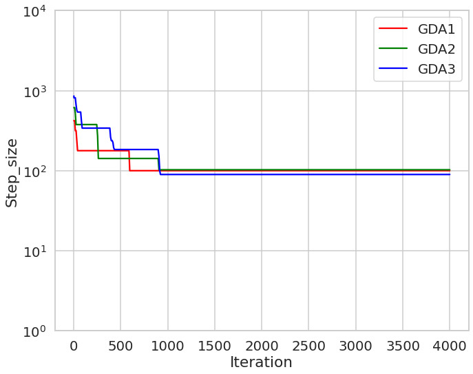
The experiments are performed with the dataset including $\mathbf{{N}}$ observations $(\mathbf{a}_{i},b_{i})\in\mathbb{R}^{d}\times\mathbb{R},i=1,\ldots,n.$ The cross-entropy loss function for multi-variable logistic regression is given by $J(x)=-\sum_{i=1}^{\mathbf{N}}\big{(}b_{i}\log\left(\sigma\left(-{x}^{T}\mathbf{a}_{i}\right)\right)+(1-b_{i})\log\left(1-\sigma\left(-{x}^{T}\mathbf{a}_{i}\right)\right)\big{)},$ where $\sigma$ is the sigmoid function. Associated with $\ell_{2}$ -regularization, we get the regularized loss function $\bar{J}(x)=J(x)+\frac{1}{2\mathbf{N}}\|x\|^{2}.$ The Lipschitz coefficient $L$ is estimated by $\frac{1}{2\mathbf{N}}(\|A\|^{2}/2+1),$ where $A=\left(a_{1}^{\top},\ldots,a_{n}^{\top}\right)^{\top}.$ We compare the algorithms for training the logistic regression problem by using datasets Mushrooms and W8a (see in Malitsky ). The GDA method is compared to the GD algorithm with a step size of $1/L$ and Nesterov’s accelerated method. The computational results are shown in Fig. 3 and Fig. 4 respectively. The figures suggest that Algorithm GDA outperforms Algorithm GD and Nesterov’s accelerated method in terms of objective function values during iterations. In particular, Fig. 4 shows the change of the objective function values according to different $\kappa$ coefficients. In this figure, the notation “GDA_0.75” respects to the case $\kappa=0.75.$ Fig. 5 presents the reduction of step-sizes from an initial step-size with respect to the results in Fig. 4.

5.3 Neural networks for classification

In order to provide an example of how the proposed algorithm can be implemented into a neural network training model, we will use the standard ResNet-18 architectures that have been implemented in PyTorch and will train them to classify images taken from the Cifar10 dataset downloaded at https://www.cs.toronto.edu/ kriz/cifar.html, while taking into account the cross-entropy loss. In the studies with ResNet-18, we made use of Adam’s default settings for its parameters.

For training this neural network model, we use the stochastic variation of the GDA method (Algorithm SGDA) to compare to Stochastic Gradient Descent (SGD) algorithms. The computational outcomes shown in Fig. 6 and Fig. 7 reveal that Algorithm SGDA outperforms Algorithm SGD in terms of testing accuracy and train loss over iterations.

6 Conclusion

We proposed a novel easy adaptive step-size process in a wide family of solution methods for optimization problems with non-convex objective functions. This approach does not need any line-searching or prior knowledge, but rather takes into consideration the iteration sequence’s behavior. As a result, as compared to descending line-search approaches, it significantly reduces the implementation cost of each iteration. We demonstrated technique convergence under simple assumptions. We demonstrated that this new process produces a generic foundation for optimization methods. The preliminary results of computer experiments demonstrated the new procedure’s efficacy.

Availability of data and materials

The data that support the findings of this study are available from the corresponding author, upon reasonable request.

Acknowledgments

This work was supported by Vietnam Ministry of Education and Training.

References

(1) Bauschke, H.H., Combettes, P.L.: Convex analysis and monotone operator theory in hilbert spaces. Springer, New York (2011)
(2) Boyd, S.P., Vandenberghe, L.: Convex Optimization. Cambridge University Press, Cambridge (2009)
(3) Rockafellar, R.T.: Convex analysis. Princeton University Press, Princeton, New Jersey (1970)
(4) Bian, W. , Ma, L., Qin, S., Xue, X.: Neural network for nonsmooth pseudoconvex optimization with general convex constraints. Neural Networks 101, 1-14 (2018).
(5) Cevher, V., Becker, S., Schmidt, M.: Convex optimization for big data. Signal Process. Magaz. 31, 32–43 (2014)
(6) Dennis, J.E., Schnabel, R.B.: Numerical methods for unconstrained optimization and nonlinear equations. Prentice-Hall, New Jersey (1983).
(7) Ferreira, O. P., Sosa, W. S.: On the Frank–Wolfe algorithm for non-compact constrained optimization problems. Optimization 71(1), 197-211 (2022).
(8) Hu, Y., Li, J., Yu, C.K.: Convergence Rates of Subgradient Methods for Quasiconvex Optimization Problems. Computational Optimization and Applications 77, 183–212 (2020).
(9) Kiwiel, K.C.: Convergence and efficiency of subgradient methods for quasiconvex minimization. Math. Program., Ser. A 90, 1–25 (2001).
(10) Konnov, I.V.: Simplified versions of the conditional gradient method. Optimization 67(12), 2275-2290 (2018).
(11) Lan, G.H.: First-order and Stochastic Optimization Methods for Machine Learning. Springer Series in the Data Sciences, Springer Nature Switzerland (2020)
(12) Liu, N., Wang, J., Qin, S.: A one-layer recurrent neural network for nonsmooth pseudoconvex optimization with quasiconvex inequality and affine equality constraints. Neural Networks 147, 1-9 (2022).
(13) Malitsky, Y., Mishchenko, K.: Adaptive Gradient Descent without Descent. Proceedings of Machine Learning Research 119, 6702-6712 (2020).
(14) Mangasarian, O.: Pseudo-convex functions. Siam Control 8, 281-290 (1965)
(15) Nesterov, Y.: Introductory lectures on convex optimization: A basic course 87, Springer Science & Business Media (2013).
(16) Xu, H.K.: Iterative algorithms for nonlinear operators. J. London Math. Soc. 66, 240-256 (2002)
(17) Yu, C.K., Hu, Y., Yang, X., Choy, S. K.: Abstract convergence theorem for quasi-convex optimization problems with applications. Optimization 68(7), 1289-1304 (2019).
(18) Wang,Y., Li, X., Wang, J.: A neurodynamic optimization approach to supervised feature selection via fractional programming. Neural Networks 136, 194–206 (2021).

	$\displaystyle\\|x^{k+1}-z\\|^{2}$	$\displaystyle=\\|x^{k}-z\\|^{2}-\\|x^{k+1}-x^{k}\\|^{2}+2\left\langle x^{k+1}-x^{k},x^{k+1}-z\right\rangle$
		$\displaystyle\leq\\|x^{k}-z\\|^{2}-\\|x^{k+1}-x^{k}\\|^{2}+2\lambda_{k}\left\langle\nabla f(x^{k}),z-x^{k+1}\right\rangle.$		(8)