Selector-Enhancer: Learning Dynamic Selection of Local and Non-local Attention Operation for Speech Enhancement
Abstract
Attention mechanisms, such as local and non-local attention, play a fundamental role in recent deep learning based speech enhancement (SE) systems. However, natural speech contains many fast-changing and relatively brief acoustic events, therefore, capturing the most informative speech features by indiscriminately using local and non-local attention is challenged. We observe that the noise type and speech feature vary within a sequence of speech and the local and non-local operations can respectively extract different features from corrupted speech. To leverage this, we propose Selector-Enhancer, a dual-attention based convolution neural network (CNN) with a feature-filter that can dynamically select regions from low-resolution speech features and feed them to local or non-local attention operations. In particular, the proposed feature-filter is trained by using reinforcement learning (RL) with a developed difficulty-regulated reward that is related to network performance, model complexity, and “the difficulty of the SE task”. The results show that our method achieves comparable or superior performance to existing approaches. In particular, Selector-Enhancer is potentially effective for real-world denoising, where the number and types of noise are varies on a single noisy mixture.
1 Introduction
Speech enhancement (SE) aims at separating the underlying high quality and intelligently speech s from a noise-corrupted speech signal , where n represents additive noise. For many applications such as mobile communication and hearing aids, SE algorithms are restricted to operate with low latency and often also to use only single-channel inputs. With the recent advances in supervised learning, deep neural networks (DNNs) have become state-of-the-art for single-channel SE. They typically operate in the short-time Fourier transform (STFT) domain and estimate the target clean speech from the noisy signal via direct spectral mapping (Xu et al. 2013) or time-frequency masking (Wang, Narayanan, and Wang 2014).
Several studies have shown the efficiency of local processing by convolutional neural networks (CNNs) for STFT-domain SE, which are structurally well-suited to focus on local patterns such as harmonic structures in the speech spectra (Park and Lee 2017). However, the speech also exhibits non-linguistic long-term dependencies, such as gender, dialect, speaking rating, and emotional state (Bengio, Simard, and Frasconi 1994). For aggregating more informative speech features, several strategies are proposed, such as encoder-decoder architecture (Park and Lee 2017), dilated convolutions (Pirhosseinloo and Brumberg 2019) or applying long-short term memory (LSTM) networks (Tan and Wang 2018; Oostermeijer, Wang, and Du 2021), to enlarge the receptive field.
Furthermore, the non-local operation (Wang et al. 2018a), which takes the advantage of self-similarity within the whole speech to recover a local speech segment, is effective to establish the long-range dependence based on time-frequency (T-F) units of speech spectra. However, T-F units of noisy speech are usually corrupted, therefore, establishing the correlation between T-F units is unreliable, especially when speech is heavily corrupted. Besides, the non-local operation has computational complexity for a sequence length of , which increases the computational burden for the SE model, hence the practical usage is limited. In addition to non-local attention, local attention processes the local neighborhood, which scales more informative feature regions with “high attention” while putting “low attention” to other feature regions and achieving a linear complexity to the input feature. However, local attention is unable to extract speech global information that is important to speech enhancement tasks, due to the limited receptive field.
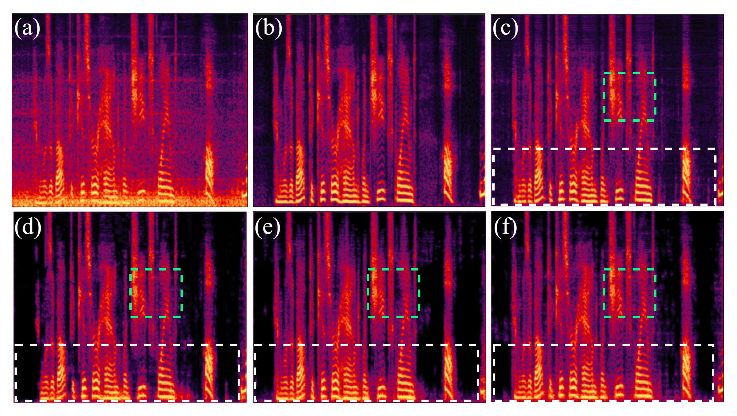
According to the above analysis, local and non-local attentions have shortcomings and merits. Figure 1(d) and Figure 1(e) show an example enhanced spectrogram processed by local and non-local attention-based SE models. The local attention-based speech enhancement model failed to process the noise component in the green dotted box. In contrast, the non-local attention-based system insufficiently removes the noise component in the white dotted box. However, integrating both attentions indiscriminately is a challenge to keep their merits while avoiding their shortcomings. For example, as shown in Figure 1(f), the SE system by directly applying local and non-local attention operations still failed to remove the noise component in the green box while remaining the low-frequency noise component in the white box.
In this study, we propose Selector-Enhancer, a novel framework that jointly processes different regions of a noisy speech spectrogram via local and non-local attention operation with the guidance of adjacent features. Particularly, a feature-filter is proposed and is trained together with dual-attention based CNN. The feature-filter first predicts a low-resolution dispatch policy mask, in which each time-frequency (T-F) unit represents a policy for a region in the input noisy spectrogram. After that, the features of different regions are sent to specific attention operations (local or non-local attention) according to the corresponding policy on the predicted mask. Since the feature selection is non-differentiable, the feature filter is trained in a reinforcement learning (RL) framework driven by a reward to achieve a good complexity-performance trade-off.
In a nutshell, the contributions of our work are three-fold111Code is available at: https://github.com/XinmengXu/Selector
-Enhancer.
-
•
We propose a novel SE framework for making a trade-off between local and non-local attention operations by introducing a feature-filter that predicts a policy mask to select the feature of different spectrogram regions and to send to specific attention operations.
-
•
We develop a difficulty-regulated reward, which is related to performance, complexity, and “the difficulty of the SE task”. Specifically, the difficulty is made by the loss function, since the high loss denotes the high difficulty of the SE task.
-
•
The proposed Selector-Enhancer achieves comparable and superior performance to recent approaches with faster speed and is particularly effective when noise distribution is variant within a speech sequence.
2 Related Work
2.1 Non-local Attention
Long-range dependencies are important prior to SE, and this prior can be effectively obtained by non-local attention operation, which calculates the mutual similarity between T-F units in each frame, which is helpful for capturing the global information in the frequency domain with a slightly increased computing complexity. In general, non-local attention is defined as follows (Wang et al. 2018b):
| (1) |
where and , respectively, represent the input and output tensor of the operation with the same size, denotes the pairwise function to calculate the correlation between the locations of the feature map, signifies the unary input function for information transform, and is a normalization factor.
Recently, deep neural networks (DNNs) have been prevalent in the community of SE, and non-local attention-based SE models have been proposed for modeling long-term dependencies of speech signals. In (Li et al. 2019a), embedding function is a convolutional layer that can be viewed as a linear embedding function, and dot product, i.e., is applied to compute the similarity between query and keys. However, non-local attention is unreliable when speech is heavily corrupted and colored noise is contained in the background mixture. In addition, a transformer with Gaussian-weighted non-local attention is proposed (Kim, El-Khamy, and Lee 2020), whose attention weights are attenuated according to the distance between correlated T-F units. The attenuation is determined by the Gaussian variance which can be learned during training. While all these methods demonstrate the benefits of non-local attention, their approach is unreliable when speech is heavily corrupted and has high computational costs.

2.2 Local Attention
Local attention focuses on the important speech components in an audio stream with “high attention” while perceiving the unimportant region (e.g., noise or interference) in “low attention”, according to the past and current time frame, thus adjusting the focal point over time. In (Hao et al. 2019), a lightweight casual transformer with local self-attention is proposed for real-time SE in computation resource-limited environments. Local attention based RNN-LSTM (Oostermeijer, Wang, and Du 2021) is proposed for superior SE performances by modeling important sequential information, in which the RNN model learns the weights of past input features implicitly when predicting an enhanced frame, the attention mechanism calculates correlations between past frames and the current frame to be enhanced and give weights to past frames explicitly. Compared with non-local attention, local attention is more suitable for real-time settings and more lightweight (Hao et al. 2019; Oostermeijer, Wang, and Du 2021), since they do not rely on future information. However, compared with non-local operations, the main drawback of the local attention mechanism during SE is the relatively small receptive field.
2.3 Dynamic Networks
Dynamic networks are effective to achieve a trade-off between speech and performance in different tasks. Recently, several approaches (Wu et al. 2018; Shalit, Johansson, and Sontag 2017; Yang et al. 2022) are applied to dynamic networks to reduce the computational cost in ResNet by dynamically skipping some residual blocks. Although the aforementioned methods mainly focus on a single task, a routing network (Rosenbaum, Klinger, and Riemer 2018) is developed to facilitate multi-task learning, and their method seeks an appropriate network path for each specific task. Existing dynamic networks successfully explore the route policy that depends on either the task to address. However, we aim at selecting different regions of input speech spectrogram to send to specific attention operations, in which noise information (noise type and signal-to-noise ratio (SNR)) and speech information (speaker identity and speech content) have a weighty influence on the performance and they should be both considered in the selection operation.
3 Methodology
Our task is to recover a clean speech s from a noisy observation . We propose Selector-Enhancer that can process each noisy observation according to its speech and noise features through a specific attention mechanism. Figure 2 gives a detailed illustration of the Selector-Enhancer framework. The Selector-Enhancer takes the noisy raw waveform and firstly transforms into a short-time Fourier transform (STFT) spectrogram, denoted by in Figure 2. The output of Selector-Enhancer is clean spectrogram , and then transforms into raw waveform through inverse STFT.
3.1 Architecture of Selector-Enhancer
We aim to design a framework that can offer different attention mechanism options for SE. To this end, as shown in Figure 2, Selector-Enhancer is composed of 3 convolutional blocks at the start- and end-point for extracting features and reconstructing the target speech, and dynamic blocks in the middle. Each convolutional block contains a stacked 2D convolutional layer which is followed by batch normalization, and exponential linear unit (ELU). Additionally, skip connections are utilized to concatenate the output of each convolutional block to the input of the corresponding deconvolutional block.
In the -th dynamic block , there is a shared path containing two convolutional blocks for extracting deeper speech features, which every feature map should pass through. Paralleling the shared path, a feature-filter generates a probabilistic distribution of plausible paths for selection by each T-F unit of the input feature map. Following the shared path, there are two paths for local and non-local attention denoted by and . According to the output of the feature-filter, the path with the highest probability is activated, where the path index is represented by action . Since the path selection is for every T-F unit rather than a feature map, the action is a two-channel mask rather than a scalar. The first channel implies the regions that go through the path for local attention, and similarly, the second channel corresponds to the path for non-local attention. The whole process is formulated as:
| (2) | ||||
where and represent the input and output of the -th dynamic block, respectively, and denotes the decoder of dynamic block. Note that “” denotes the element-wise multiplication, and each channel of feature performs the same element-wise multiplication with mask . Specially, the mask utilizes two branches to generate a 1-D frequency-dimension mask and a 1-D time-frame mask in parallel, then combines them with a matrix multiplication to obtain the final 2-D mask.


3.2 Local and Non-local Attention
The local and non-local attention operations are demonstrated as follows:
Local Attention. Inspired by (Li et al. 2019b), we employ a channel-wise attention mechanism to design the local attention to perform channel selection with multiple sizes of the receptive field. The detailed architecture of the local attention is shown in Figure 3. In the local attention, we utilized two branches to carry different numbers of convolution layers to generate feature maps with different sizes of receptive filed. The channel-wise attention is independently performed on these two outputs. As illustrated in Figure 3, given input feature I, two-layer convolutional blocks and four-layer convolutional blocks generate their output and in a paralleled manner:
| (3) |
where and refer to functions of the two and four convolutional blocks. After getting and , the scaled feature is obtained in the following steps:
| (4) |
where and refer to two independent fully-connected layers. Finally, the final output J can be obtained as follows:
| (5) |
where is the function of one layer convolutional block.
Non-local Attention. The detailed architecture of non-local attention is shown in Figure 4. Given the input I, we adopt three independent convolutional layers with trainable parameters as embedding functions. These three embedding functions are denoted as , , and . They are used to generate the query (Q), key (K), and value (V). The embedding process does not change the size of the input, which can be defined as follows:
| (6) |
The distance matrix denoted by A can be efficiently calculated as by dot product:
| (7) |
The output of non-local attention operation W, defined by Eq.(1), is calculated by the matrix multiplication between A and V. Finally, W is fed into a convolutional operation to generate the output J.
3.3 Feature Filter
The architecture of the feature filter is illustrated in Figure 2, which is the key component to achieve the selection operation. The feature filter contains three convolutional blocks, two LSTMs for capturing the correlations of the feature filter in different dynamic blocks, and a convolutional block followed by a sigmoid activation function. In addition, the selection operation is non-differentiable, thus we adopt Markov Decision Process (MDP) and reinforcement learning (RL) to train the feature filter. The state and action of this MDP and the developed difficulty-regulated reward for the feature filter training are clarified as follows:
State and Action. In the -th dynamic block, the state include the input feature and the hidden state of LSTM . Given the state , the feature filter produces a distribution of selection that can be expressed as . In the training phase, the action is sampled from the probabilistic distribution, referred to as . While in the testing phase, the action is determined by the highest probability, i.e., , in which the action is the two-channel mask that is described in Section 3.1.
Difficulty-regulated Reward. In the RL framework, the feature filter is trained to maximize a cumulative reward. In this paper, for the attention selection, we develop a difficulty-regulated reward, which considers the network performance, complexity, and difficulty of the task. The reward at -th dynamic block is expressed as:
| (8) |
where is the reward penalty for selecting a path in one dynamic block. In addition, the performance gain in terms of L2 loss. The difficulty is denoted by is formulated as:
| (9) |
where is the Mean Square Error (MSE) loss function and is a threshold. As approaches zero, the difficult decreases, indicating the input noisy mixture is easy to enhance.
3.4 Implementation
The Selector-Enhancer is composed of dual-attention based CNN and feature filter, and the training process of Selector-Enhancer consists of two stages. In the first stage, we train a dual-attention based CNN pre-trained model with a random policy mask. In the second stage, we train the feature filter and dual-attention based CNN together.
Stage 1. We train the dual-attention based CNN pre-trained model with a randomly generated policy mask. In this study, we design a loss function by using MSE loss constrains the output to have reasonable quality.
Stage 2. We train the local and non-local based CNN and feature filter together. We train the feature filter using the REINFORCE algorithm (Williams 1992), as illustrated in Algorithm 1. The parameters of the feature-filter and learning rate are denoted by and , respectively.

| Case Index | 0 (default) | 1 | 2 | 3 | 4 | 5 | 6 | 7 | 8 | 9 |
| Local Attention | ||||||||||
| Non-local Attention | ||||||||||
| Concatenation | ||||||||||
| Selective Network (Li et al. 2019b) | ||||||||||
| Feature-Filter (Proposed) | ||||||||||
| Number of DB | 4 | 4 | 4 | 4 | 4 | 4 | 3 | 2 | 1 | 5 |
| PESQ | 3.09 | 2.63 | 2.66 | 2.82 | 2.99 | 2.36 | 3.02 | 2.94 | 2.87 | 3.11 |
| STOI () | 93.41 | 87.15 | 87.47 | 91.10 | 92.28 | 78.39 | 92.76 | 91.33 | 91.01 | 93.38 |
| Parameters | 2.37M | 1.98M | 2.27M | 2.38M | 2.55M | 2.15M | 2.24M | 2.03M | 1.81M | 2.57M |
4 Experiments
4.1 Datasets
To evaluate the proposed Selector-Enhancer, we use two types of datasets: VoiceBank + DEMAND and AVSpeech + AudioSet.
VoiceBank + DEMAND: This is an open dataset proposed by (Yin et al. 2020). The pre-scaled subset of VoiceBank (Valentini-Botinhao et al. 2016) provided by is used to train the Selector-Enhancer. We randomly select 40 male speakers and 40 female speakers from the total of 84 speakers (42 male and 42 female), and each speaker pronounced around 4000 utterances. Therefore, the clean data contained 320,000 utterances in total (16,000 male utterances and 16,000 female utterances). Next, we mix 32,000 utterances with noise from DEMAND (Thiemann, Ito, and Vincent 2013) in dB signal-to-noise ratio (SNR) levels. In addition, we set aside 200 clean utterances from the training set to create a validation set. Test data are generated by mixing 200 utterances selected from the remained 4 untrained speakers (50 each) with noise from DEMAND at three SNR levels dB.
AVSpeech+AudioSet: This is a large dataset proposed by (Ephrat et al. 2018). The clean dataset AVSpeech is collected from Youtube, containing 4700 hours of video segments with approximately 150,000 distinct speakers spanning a wide variety of people languages. The noisy speech is a mixture of the above clean speech segments with AudioSet (Gemmeke et al. 2017) that contains a total of more than 1.7 million 10-second segments of 526 kinds of noise. The noisy speech is synthesized by a weighted linear combination of speech segments and noise segments (Yin et al. 2020):
| (10) |
where and are 4-second segments randomly sampled from the speech and noise dataset. In our experiment, 10,000 segments were randomly sampled from the AVSpeech dataset for the training set and 500 segments for the validation dataset. Because of the wide energy distribution in both datasets, the created noisy speech dataset has a wide range of SNR.
For the test dataset, we randomly select 840 utterances from 84 speakers in WSJ0 SI-84 dataset (Paul and Baker 1992) and mingle with unknown types of non-stationary noises from NOISEX92 (Varga and Steeneken 1993) under three SNR levels dB. The choice of the training set and test set is to let the Selector-Enhancer adapt to different speakers and different acoustic environments.
4.2 Experimental Setup
As for the number of dynamic blocks, we use for a fair comparison with the baseline methods. The threshold of difficulty and the reward penalty are, respectively, set to and based on the specific task. Specifically, when the noise corruption is severe, the threshold and reward penalty is required to be larger. In the first training stage, the coefficient of intermediate loss is set to 0.5. All the utterances are sampled at 16 kHz and features are extracted by using frames of length 512 with frame-shift of 256, and Hann windowing followed by STFT of size K = 512 with respective zero-padding. We train the model with a minibatch size of 16. We use Adam as an optimizer and implement our method on Pytorch.
In our experiments, the performance is assessed by using standard speech enhancement metrics short-term objective intelligibility (STOI), and perceptual evaluation of speech quality (PESQ). STOI typically has a value range from 0 to 1 and can be interpreted as percent correct, and PESQ has a value range from -0.5 to 4.5.
4.3 Ablation Study
We show the ablation study in Table 1 to investigate the effect of different components in Selector-Enhancer. Note that Case 0 denotes the proposed basic Selector-Enhancer with the default setting. In the ablation study, we compare our method with several models: 1) Case 1: we remove all non-local attention mechanisms, 2) Case 2: we remove all local attention mechanisms, 3) Case 3: We remove the feature filters and adopt concatenation operation to fuse results of local and non-local operations, 4) Case 4: we remove feature filters and adopt selection network (Li et al. 2019b) to fuse results of local and non-local operations, 5) Case 5: we remove all components of Selector-Enhancer. We show the detailed analysis of ablation below.
Local Attention Compare with Case 3, Case 2 removes all local attention mechanisms. According to Table 1, we find that Case 3 improves PESQ by 0.16 and STOI by over Case 2. The obvious performance decrease in Case 2 indicates the positive effect of the local attention operation. In addition, we remove both local and non-local attention mechanisms in Case 5. Case 1 achieves 0.30 PESQ improvement and STOI improvement over Case 5. The performance comparison between Case 1 and Case 5 illustrates the necessity of the local operation for SE.
Non-local Attention To verify the effect of non-local attention, we also provide two groups of comparison. Comparing Case 1 and Case 3, one can observe that local attention mechanisms produce 0.19 PESQ gains and STOI gains together with local attention mechanisms. What is more, From Case 1 to Case 5, the non-local attention mechanisms contribute 0.27 PESQ gains and STOI gains. Consequently, these two groups of comparison demonstrate the necessity of the non-local operation for SE.
Attention Collaboration We declare that adopting local and non-local attention directly by deep learning networks is challenging since the speech contains dynamic and fast-changing features. To verify the necessity of attention collaborative operation, we make a comparison between Case 3 and Case 4. Note that Case 4 incorporates the local and non-local attention mechanisms by adopting selective network (Li et al. 2019b). From Case 3 to Case 4, the 0.17 PESQ gains and STOI gains by Case 4 over Case 3 fully demonstrate the superiority of the collaborative operation between local and non-local attention mechanisms.
Feature-Filter To verify the necessity of our proposed feature filter, we compare Case 0 with Case 3 and Case 4 separately. The 0.27 PESQ gains and STOI gains by Case 0 over Case 3 and the 0.10 PESQ gains and STOI gains by Case 0 over Case 4 obviously indicate the effectiveness of our proposed feature filter for local and non-local attention collaboration.
In order for a better understanding of the feature-filter, we visualize the masked feature maps processed by the feature filter for local and non-local attention mechanisms and processed feature maps produced by local and non-local attention operation in Figure 5. We show that the corrupted speech components are scaled and masked by feature-filter to separately feed into local and non-local attention operations.
Number of Dynamic Blocks To study the number of dynamic blocks, we make a comparison among Cases 0, 6, 7, 8, and 9, which clearly shows that the performance increases with the number of dynamic blocks. Therefore, for a good trade-off between speed and accuracy, we use 4 dynamic blocks as our final proposed model to do comparisons to other state-of-the-art works.
| SNR | -5 dB | 0 dB | 5 dB | FLOPs (G) | Param. (M) | RTF | |||
|---|---|---|---|---|---|---|---|---|---|
| Metrics | STOI (%) | PESQ | STOI (%) | PESQ | STOI (%) | PESQ | |||
| Unprocessed | 56.32 | 1.30 | 70.95 | 1.57 | 81.33 | 1.83 | - | - | - |
| CRN (2019) | 73.36 | 1.81 | 82.27 | 2.45 | 89.27 | 2.90 | 1.16 | 2.36 | 0.52 |
| CNN-NL (2020) | 77.98 | 1.90 | 85.63 | 2.51 | 90.11 | 3.05 | 5.94 | 5.04 | 0.86 |
| T-GSA (2020) | 80.88 | 2.14 | 88.47 | 2.66 | 91.37 | 3.03 | 6.23 | 5.63 | 0.95 |
| SA-TCN (2021) | 82.47 | 2.26 | 89.89 | 2.84 | 92.73 | 3.25 | 8.85 | 5.81 | 0.91 |
| Selector-Enhancer | 83.38 | 2.36 | 91.24 | 3.03 | 94.36 | 3.37 | 2.19 | 2.37 | 0.63 |
4.4 System Comparison
We carry out the system comparison on both datasets mentioned in section 4.1.
VoiceBank+DEMAND: We train the proposed Selector-Enhancer on the synthetic and commonly used dataset VoiceBank+DEMAND. The results are provided in Table 2. We compare our model with 4 recent baselines, CRN (Tan and Wang 2018), CNN-NL (Li et al. 2019a), T-GSA (Kim, El-Khamy, and Lee 2020), and SA-TCN (Lin et al. 2021). Firstly, the non-local attention based SE models like CNN-NL, T-GSA, and SA-TCN have a very large gain over the simple CNN-based SE model (CRN) in terms of STOI and PESQ. This indicates the advantage of non-local attention operations in capturing long-term dependencies. Also, Selector-Enhancer yields the best results in all conditions.
Realizing that the number of trainable parameters can not completely reflect the complexity of a model, especially for deep non-local methods. Thus we employ the floating-point operations (FLOPs), the number of trainable parameters, and real-time factor (RTF) to evaluate the complexity of different methods. The complexity analysis of several representative methods is reported in Table 2. The proposed Selector-Enhancer has an attractive complexity and low computational costs and achieves quite promising performance.
| Test SNR | -5 dB | 0 dB | 5 dB | |||
| Metrics | STOI | PESQ | STOI | PESQ | STOI | PESQ |
| Mixture | 57.99 | 1.18 | 57.99 | 1.18 | 90.03 | 2.06 |
| U-Net | 72.92 | 1.76 | 87.01 | 2.06 | 91.85 | 2.37 |
| GRN | 74.96 | 1.81 | 88.62 | 2.19 | 91.72 | 2.44 |
| PHASEN | 74.77 | 2.47 | 89.89 | 2.93 | 93.70 | 3.09 |
| TFT-Net | 76.94 | 2.47 | 90.33 | 2.93 | 93.70 | 3.11 |
| Selector-Enhancer | 78.33 | 2.52 | 91.19 | 3.06 | 94.27 | 3.15 |
AVSpeech+AudioSet: On this large dataset, we compare the Selector-Enhancer with several state-of-the-art methods,i.e., U-Net (Park and Lee 2017), GRN (Pirhosseinloo and Brumberg 2019), PHASEN (Yin et al. 2020), and TFT-Net (Tang et al. 2021). The results in Table 3 demonstrate that the Selector-Enhancer outperforms these state-of-the-art methods and also indicate that the Selector-Enhancer can be generalized to various speakers and various kinds of noisy environments.


To demonstrate the effectiveness and flexibility of the Selector-Enhancer, we further explore and apply the Selector-Enhancer to circumstances when multiple noise types are included in a noisy background. We randomly select 150 clean utterances from the test set and 3 challenging noises, babble (B), factory (F), and cafeteria (C) from NOISEX92, which are explained in Section 4.1, to produce the multiple types of noises with clean utterances at -5 dB, 0 dB, and 5 dB SNR levels. Figure 6 shows the STOI and PESQ results over three mentioned SNR levels on multiple noise types, where B, F, and C represent babble, factory, and cafeteria noise types, respectively. According to the Table, we observe that the results using 1, 2, and 3 noise types in the noisy background are comparable, although the STOI and PESQ scores are decreasing when the number of noise types is increase.
5 Conclusion
In this paper, we propose Selector-Enhancer that enables attention selection for each speech feature region. Specifically, Selector-Enhancer contains a dual-attention based CNN and a feature filter. The dual-attention based CNN offers options for local and non-local attention mechanisms to address different types of noisy mixtures while the feature-filter selects the optimal regions of speech spectra to feed into the specific attention mechanisms. Comprehensive ablation studies have been carried out, justifying almost every design choice we have made in Selector-Enhancer. Experimental results show that the proposed method is capable of superior performance in SE by outperforming the state-of-the-art methods with fewer computational costs.
References
- Bengio, Simard, and Frasconi (1994) Bengio, Y.; Simard, P.; and Frasconi, P. 1994. Learning long-term dependencies with gradient descent is difficult. IEEE transactions on neural networks, 5(2): 157–166.
- Ephrat et al. (2018) Ephrat, A.; Mosseri, I.; Lang, O.; Dekel, T.; Wilson, K.; Hassidim, A.; Freeman, W. T.; and Rubinstein, M. 2018. Looking to listen at the cocktail party: a speaker-independent audio-visual model for speech separation. ACM Transactions on Graphics (TOG), 37(4): 1–11.
- Gemmeke et al. (2017) Gemmeke, J. F.; Ellis, D. P.; Freedman, D.; Jansen, A.; Lawrence, W.; Moore, R. C.; Plakal, M.; and Ritter, M. 2017. Audio set: An ontology and human-labeled dataset for audio events. In 2017 IEEE international conference on acoustics, speech and signal processing (ICASSP), 776–780. IEEE.
- Hao et al. (2019) Hao, X.; Shan, C.; Xu, Y.; Sun, S.; and Xie, L. 2019. An attention-based neural network approach for single channel speech enhancement. In ICASSP 2019-2019 IEEE International Conference on Acoustics, Speech and Signal Processing (ICASSP), 6895–6899. IEEE.
- Kim, El-Khamy, and Lee (2020) Kim, J.; El-Khamy, M.; and Lee, J. 2020. T-gsa: Transformer with gaussian-weighted self-attention for speech enhancement. In ICASSP 2020-2020 IEEE International Conference on Acoustics, Speech and Signal Processing (ICASSP), 6649–6653. IEEE.
- Li et al. (2019a) Li, X.; Li, Y.; Li, M.; Xu, S.; Dong, Y.; Sun, X.; and Xiong, S. 2019a. A Convolutional Neural Network with Non-Local Module for Speech Enhancement. In Interspeech, 1796–1800.
- Li et al. (2019b) Li, X.; Wang, W.; Hu, X.; and Yang, J. 2019b. Selective kernel networks. In Proceedings of the IEEE/CVF Conference on Computer Vision and Pattern Recognition, 510–519.
- Lin et al. (2021) Lin, J.; van Wijngaarden, A. J. d. L.; Wang, K.-C.; and Smith, M. C. 2021. Speech enhancement using multi-stage self-attentive temporal convolutional networks. IEEE/ACM Transactions on Audio, Speech, and Language Processing, 29: 3440–3450.
- Oostermeijer, Wang, and Du (2021) Oostermeijer, K.; Wang, Q.; and Du, J. 2021. Lightweight Causal Transformer with Local Self-Attention for Real-Time Speech Enhancement. In Proc. Interspeech 2021, 2831–2835.
- Park and Lee (2017) Park, S. R.; and Lee, J. W. 2017. A Fully Convolutional Neural Network for Speech Enhancement. Proc. Interspeech 2017, 1993–1997.
- Paul and Baker (1992) Paul, D. B.; and Baker, J. 1992. The design for the Wall Street Journal-based CSR corpus. In Speech and Natural Language: Proceedings of a Workshop Held at Harriman, New York, February 23-26, 1992.
- Pirhosseinloo and Brumberg (2019) Pirhosseinloo, S.; and Brumberg, J. S. 2019. Monaural Speech Enhancement with Dilated Convolutions. In INTERSPEECH, 3143–3147.
- Rosenbaum, Klinger, and Riemer (2018) Rosenbaum, C.; Klinger, T.; and Riemer, M. 2018. Routing Networks: Adaptive Selection of Non-Linear Functions for Multi-Task Learning. In International Conference on Learning Representations.
- Shalit, Johansson, and Sontag (2017) Shalit, U.; Johansson, F. D.; and Sontag, D. 2017. Estimating individual treatment effect: generalization bounds and algorithms. In International Conference on Machine Learning, 3076–3085. PMLR.
- Tan and Wang (2018) Tan, K.; and Wang, D. 2018. A Convolutional Recurrent Neural Network for Real-Time Speech Enhancement. In Interspeech, volume 2018, 3229–3233.
- Tang et al. (2021) Tang, C.; Luo, C.; Zhao, Z.; Xie, W.; and Zeng, W. 2021. Joint time-frequency and time domain learning for speech enhancement. In Proceedings of the Twenty-Ninth International Conference on International Joint Conferences on Artificial Intelligence, 3816–3822.
- Thiemann, Ito, and Vincent (2013) Thiemann, J.; Ito, N.; and Vincent, E. 2013. The Diverse Environments Multi-channel Acoustic Noise Database (DEMAND): A database of multichannel environmental noise recordings. In Proceedings of Meetings on Acoustics ICA2013, volume 19, 035081. Acoustical Society of America.
- Valentini-Botinhao et al. (2016) Valentini-Botinhao, C.; Wang, X.; Takaki, S.; and Yamagishi, J. 2016. Investigating RNN-based speech enhancement methods for noise-robust Text-to-Speech. In SSW, 146–152.
- Varga and Steeneken (1993) Varga, A.; and Steeneken, H. J. 1993. Assessment for automatic speech recognition: II. NOISEX-92: A database and an experiment to study the effect of additive noise on speech recognition systems. Speech communication, 12(3): 247–251.
- Wang et al. (2018a) Wang, X.; Girshick, R.; Gupta, A.; and He, K. 2018a. Non-local neural networks. In Proceedings of the IEEE conference on computer vision and pattern recognition, 7794–7803.
- Wang et al. (2018b) Wang, X.; Girshick, R.; Gupta, A.; and He, K. 2018b. Non-local neural networks. In Proceedings of the IEEE conference on computer vision and pattern recognition, 7794–7803.
- Wang, Narayanan, and Wang (2014) Wang, Y.; Narayanan, A.; and Wang, D. 2014. On training targets for supervised speech separation. IEEE/ACM transactions on audio, speech, and language processing, 22(12): 1849–1858.
- Williams (1992) Williams, R. J. 1992. Simple statistical gradient-following algorithms for connectionist reinforcement learning. Machine learning, 8(3): 229–256.
- Wu et al. (2018) Wu, Z.; Nagarajan, T.; Kumar, A.; Rennie, S.; Davis, L. S.; Grauman, K.; and Feris, R. 2018. Blockdrop: Dynamic inference paths in residual networks. In Proceedings of the IEEE Conference on Computer Vision and Pattern Recognition, 8817–8826.
- Xu et al. (2013) Xu, Y.; Du, J.; Dai, L.-R.; and Lee, C.-H. 2013. An experimental study on speech enhancement based on deep neural networks. IEEE Signal processing letters, 21(1): 65–68.
- Yang et al. (2022) Yang, C.-H. H.; Hung, I.-T. D.; Ouyang, Y.; and Chen, P.-Y. 2022. Training a resilient q-network against observational interference. In Proceedings of the AAAI Conference on Artificial Intelligence, volume 36, 8814–8822.
- Yin et al. (2020) Yin, D.; Luo, C.; Xiong, Z.; and Zeng, W. 2020. Phasen: A phase-and-harmonics-aware speech enhancement network. In Proceedings of the AAAI Conference on Artificial Intelligence, volume 34, 9458–9465.