Segment Anything Model for Medical Images?
Abstract
The Segment Anything Model (SAM) is the first foundation model for general image segmentation. It has achieved impressive results on various natural image segmentation tasks. However, medical image segmentation (MIS) is more challenging because of the complex modalities, fine anatomical structures, uncertain and complex object boundaries, and wide-range object scales. To fully validate SAM’s performance on medical data, we collected and sorted 53 open-source datasets and built a large medical segmentation dataset with 18 modalities, 84 objects, 125 object-modality paired targets, 1050K 2D images, and 6033K masks. We comprehensively analyzed different models and strategies on the so-called COSMOS 1050K dataset. Our findings mainly include the following: 1) SAM showed remarkable performance in some specific objects but was unstable, imperfect, or even totally failed in other situations. 2) SAM with the large ViT-H showed better overall performance than that with the small ViT-B. 3) SAM performed better with manual hints, especially box, than the Everything mode. 4) SAM could help human annotation with high labeling quality and less time. 5) SAM was sensitive to the randomness in the center point and tight box prompts, and may suffer from a serious performance drop. 6) SAM performed better than interactive methods with one or a few points, but will be outpaced as the number of points increases. 7) SAM’s performance correlated to different factors, including boundary complexity, intensity differences, etc. 8) Finetuning the SAM on specific medical tasks could improve its average DICE performance by 4.39% and 6.68% for ViT-B and ViT-H, respectively. Codes and models are available at: https://github.com/yuhoo0302/Segment-Anything-Model-for-Medical-Images. We hope that this comprehensive report can help researchers explore the potential of SAM applications in MIS, and guide how to appropriately use and develop SAM.
keywords:
\KWDSegment Anything Model, Medical Image Segmentation, Medical Object Perception1 Introduction
The emergence of large language models such as ChatGPT333https://chat.openai.com and GPT-4444https://openai.com/research/gpt-4 has sparked a new era in natural language processing (NLP), characterized by their remarkable zero-shot and few-shot generalization abilities. This progress has inspired researchers to develop similarly large-scale foundational models for computer vision (CV). The first proposed foundational CV models have been primarily based on pre-training methods such as CLIP [85] and ALIGN [46]. CLIP can recognize and understand visual concepts and details, such as object shape, texture, and color, by associating them with their corresponding textual descriptions. This allows CLIP to perform a wide range of tasks, including image classification, object detection, and even visual question answering. ALIGN can generate natural language descriptions of image regions, providing more detailed and interpretable results than traditional image-captioning approaches. DALL·E [86] was developed to generate images from textual descriptions. This model was trained on a large dataset of text-image pairs that could create a wide range of images, from photorealistic objects to surreal scenes that combine multiple concepts. However, these models have not been explicitly optimized for image segmentation, particularly medical image segmentation (MIS).
Recently, the Segment Anything Model (SAM) was proposed as an innovative foundational model for image segmentation [50]. SAM was based on the vision transformer (ViT) [24] model and trained on a large dataset with 11 million images containing 1 billion masks. The biggest highlight of SAM is its good zero-shot segmentation performance for unseen datasets and tasks. This process is driven by different prompts, e.g., points and boxes, for indicating the pixel-level semantics and region-level positions of the target objects. It has been proven to be highly versatile and capable of addressing a wide range of segmentation tasks [50].


Based on the pre-trained models of SAM, several papers have further studied its performance in different zero-shot segmentation scenarios. We roughly divide them into two categories: 1) non-medical and 2) medical applications.
1.1 SAM in Non-medical Image Applications
Two studies focused on testing SAM’s performance under the Everything mode in segmenting the camouflaged objects [97, 42]. Results showed that its performance was poor in these scenes, e.g., camouflaged animals that are visually hidden in their natural surroundings. The authors found that SAM failed to detect concealed defects in industrial scenes [42]. Ji et al. [43] explored three testing methods of the SAM (points, boxes, and everything) for various applications. Specifically, their tasks covered natural images (salient/camouflaged/transparent object segmentation, and shadow detection), agriculture (crop segmentation and pest and leaf disease monitoring), manufacturing (anomaly and surface defect detection), and remote sensing (building and road extraction). They concluded that, although SAM can achieve good performance in some scenarios, such as salient object segmentation and agricultural analysis, it produces poor results in other applications. They also validated that human prompts can effectively refine the segmentation results compared to the automatic Everything approach.
1.2 SAM in Medical Image Analysis
Ji et al. [42] assessed the SAM under the Everything mode in segmenting the lesion regions in various anatomical structures (e.g., brain, lung, and liver) and modalities (computerized tomography (CT) and magnetic resonance imaging (MRI)). The experimental results indicated that SAM was relatively proficient in segmenting organ regions with clear boundaries but may struggle to accurately identify amorphous lesion regions. Another study then evaluated the performance of SAM in some healthcare subfields (optical disc and cup, polyp, and skin lesion segmentation) using both automatic Everything and two manual Prompt (points and boxes) strategies [43]. The authors found that SAM required substantial human prior knowledge (i.e., points) to obtain relatively accurate results on these tasks. Otherwise, SAM resulted in wrong segmentation, especially when no prompts are given. In the brain extraction task using MRI, Mohapatra et al. [75] compared SAM with the brain extraction tool (BET) of the FMRIB Software Library. Quantitative results showed that the segmentation results of SAM were better than those of BET, demonstrating the potential of SAM for application in brain extraction tasks. Deng et al. [22] assessed the performance of SAM in digital pathology segmentation tasks, including tumor, non-tumor tissue and cell nuclei segmentation on whole-slide imaging. The results suggested that SAM delivers outstanding segmentation results for large connected objects. Nevertheless, it may not consistently achieve satisfactory performance for dense instance object segmentation, even with prompts of all the target boxes or 20 points per image. Zhou et al. [109] applied SAM to the polyp segmentation task using five benchmark datasets under the Everything setting. The results showed that although SAM can accurately segment the polyps in some cases, a large gap exists between SAM and the state-of-the-art methods. Additionally, Liu et al. [65] equipped the 3D Slicer software [79] with SAM to assist in the development, assessment, and utilization of SAM on medical images.
Most recently, several studies tested the SAM on 10 public MIS datasets or tasks [27, 73, 69, 103]. In [27], it was concluded that SAM’s zero-shot segmentation performance is considerably inferior to that of traditional deep learning-based methods. In Mazurowski et al. [73], the authors evaluated SAM’s performance using different numbers of point prompts. They observed that as the number of points increases, the performance of SAM converges. They also noticed that SAM’s performance is 1) overall moderate and 2) extremely unstable across different datasets and cases. Ma and Wang [69] validated that the original SAM may fail on lots of medical datasets with the mean DICE score of 58.52%. They then finetuned the SAM using medical images and found that the proposed MedSAM achieved a 22.51% improvement on DICE compared with the SAM. Wu et al. [103] adopted the Adapter technique to finetune the SAM and enhance its medical ability. Experiments validated that their proposed Medical SAM Adapter can outperform the state-of-the-art (SOTA) MIS methods (e.g., nnUnet [37]).
Although the above works investigated the performance of SAM in MIS, they had at least one of the following limitations:
-
1.
Small datasets. Previous studies have only evaluated SAM’s performance in modalities, such as MRI, CT, and digital pathology. They included a limited number of segmented objects. However, medical images contain multiple modalities and numerous anatomical structures or other objects requiring segmentation. This has limited the comprehensive analysis in the field of MIS of the above studies [42, 43, 75, 22, 109].
-
2.
Single SAM testing strategy. Most previous studies [42, 73, 109] evaluated SAM with limited or even only one type of testing mode/strategy. However, different medical objects often exhibit different characteristics and thus may have their own suitable modes for testing. The limited testing strategy may lead to inaccurate and incomplete analysis for SAM.
-
3.
Lack of comprehensive and in-depth assessments. Some of the existing works [43] only assessed the SAM via the visualization results provided by the online demo555https://segment-anything.com/demo. Additionally, some studies focused only on limited metrics (e.g., DICE or IOU) to evaluate the performance of SAM [22]. Most of the studies did not investigate SAM’s perception of medical objects. Thus, the correlation between SAM’s segmentation performance and medical objects’ attributes has not been conducted carefully [27, 73, 69].
The analysis of medical object perception is crucial. It can help the community better understand the factors that influence SAM segmentation performance (i.e., the ability to perceive medical objects), to better develop a new generation of general medical segmentation models.
In this report, we build a large medical image dataset named COSMOS 1050K, including images with 18 different modalities (see Fig. 1) and 84 objects (e.g., anatomical structures, lesions, cells, tools, etc.), to cover the entire body (see Fig. 2). This can help us comprehensively analyze and evaluate SAM’s performance on medical images. We then fully explore the different testing strategies of SAM and provide rich quantitative and qualitative experimental results to show SAM’s perception of medical objects. Finally, we deeply evaluate the correlation between SAM’s performance and the characteristics (e.g., complexity, contrast, and size) of the objects. We hope that this comprehensive report can provide the community with some insights into the future development of medical SAM.

2 Dataset
Medical images have various modalities such as CT, MRI, ultrasound (US), and X-ray. There are large domain gaps between different modalities [100], and various modalities have their advantages in visualizing specific objects, including anatomical structures and lesions [65]. To fully evaluate the generalization performance of SAM in MIS, we collected 53 public datasets and standardized them to construct the large COSMOS 1050K dataset. For the categorization system (e.g., modal categorization) of COSMOS 1050K, we referred to the official introduction of each public dataset and the recently-published study [9] (see Table 1 for more details). Fig. 1 and Fig. 2 illustrate various imaging modalities and most of the clinical segmentation objects covered in the dataset, respectively. We describe the details of COSMOS 1050K in the following two aspects, including image collection and preprocessing specification.
[b]
| Dataset Name | Description | Image Modalities |
|---|---|---|
| AbdomenCT-1K [71] | Liver, kidney, spleen and pancreas | CT |
| ACDC [7] | Left and right ventricle and left ventricular myocardium | Cine-MRI |
| AMOS 2022 [45] | Abdominal multi-organ segmentation | CT, MRI |
| AutoLaparo [101] | Integrated dataset with multiple image-based perception tasks | Colonoscopy |
| BrainPTM 2021 [2, 76] | white matter tracts | T1W MRI, DW MRI |
| BraTS20 [74, 3, 4] | Brain tumor | T1W MRI, T2W MRI, T1-GD MRI, T2-FLAIR MRI |
| CAMUS [53] | Four-chamber and Apical two-chamber heart | US |
| CellSeg Challenge-NeurIPS 2022 [70] | Cell segmentation | Microscopy |
| CHAOS [49] | Livers, kidneys and spleens | CT, T1W MRI, T2W MRI |
| CHASE-DB1 [106] | Retinal vessel segmentation | Fundus |
| Chest CT Segmentation [19] | Lungs, heart and trachea | CT |
| CRAG [25] | Colorectal adenocarcinoma | Histopathology |
| crossMoDA [92, 91] | Vestibular schwannoma | T1W MRI |
| CVC-ClinicDB [5] | Polyp | Colonoscopy |
| DRIVE [64] | Retinal vessel segmentation | Fundus |
| EndoTect 2020 [32] | Polyp | Colonoscopy |
| EPFL-EM [67] | Mitochondria and synapses segmentation | Electron Microscopy |
| ETIS-Larib Polyp DB [6, 104] | Polyp | Colonoscopy |
| FeTA [78] | Seven tissues of the infant brain | T2W MRI |
| HaN-Seg [80] | Healthy organs-at-risk near the head and neck | CT |
| I2CVB [56] | Prostate | T2W MRI |
| iChallenge-AMD [59] | Optic disc and fovea | Fundus |
| iChallenge-PALM [36] | Optic disc and lesions from pathological myopia patients | Fundus |
| IDRiD 2018 [81] | Optic disc, fovea and lesion segmentation | Fundus |
| iSeg 2019 [95] | White matter, gray matter, and cerebrospinal fluid of infant brain | T1W MRI, T2W MRI |
| ISIC 2018 [98, 17, 16] | Melanoma of skin | Dermoscopy |
| IXI [21] | Callosum | T1W MRI |
| KiPA22 [29, 28, 89, 90] | Kidney, tumor, renal vein and renal artery | CT |
| KiTS19 [31] | Kidneys and tumors | CT |
| KiTS21 [107] | Kidneys, cysts, tumors, ureters, arteries and veins | CT |
| Kvasir-Instrumen [40] | Gastrointestinal procedure instruments such as snares, balloons, etc. | Colonoscopy |
| Kvasir-SEG [41] | Gastrointestinal polyp | Colonoscopy |
| LiVScar [47] | Infarct segmentation in the left ventricle | CMR |
| LUNA16 [88] | Lungs, heart and trachea | CT |
| M&Ms [10] | Left and right ventricle and left ventricular myocardium | CMR |
| MALBCV-Abdomen [52] | Abdominal multi-organ segmentation | CT |
| Montgomery County CXR Set [39] | Lung | X-ray |
| MRSpineSeg [77] | multi-class segmentation of vertebrae and intervertebral discs | MRI |
| MSD [1, 93] | Large-scale collection of 10 Medical Segmentation Datasets | CT, MRI, ADC MRI, T1W MRI, T2W MRI, T1-GD MRI, T2-FLAIR MRI |
| NCI-ISBI 2013 [57] | Prostate (peripheral zone, central gland) | T2W MRI |
| PROMISE12 [62] | Prostate | T2W MRI |
| QUBIQ 2021 [44] | Kidney, prostate, brain growth, and brain tumor | CT, MRI, T1W MRI, T2W MRI, T1-GD MRI, T1-FLAIR MRI |
| SIIM-ACR [105, 99] | Pneumothorax segmentation | X-ray |
| SKI10 [55] | Cartilage and bone segmentation from knee data | MRI |
| SLIVER07 [30] | Liver | CT |
| ssTEM [11] | Neuronal structures | Electron Microscopy |
| STARE [34, 33] | Retinal vessel segmentation | Fundus |
| TN-SCUI 2020 [108] | Thyroid nodule | US |
| TotalSegmentator [102] | Multiple anatomic structures segmentation(27 organs, 59 bones, 10 muscles, and 8 vessels) | CT |
| VerSe19 [87] | Spine or vertebral segmentation | CT |
| VerSe20 [66, 61] | Spine or vertebral segmentation | CT |
| Warwick-QU [94] | Gland segmentation | Histopathology |
| WORD [68] | Abdominal multi-organ segmentation | CT |
| 4C2021 C04 TLS01 [20] | Throat and hypopharynx cancer lesion area | CT |


2.1 Dataset Collection
Medical images cover a wide range of object types, such as brain organs and tumors [93, 92, 4, 95, 80], lungs and hearts [7, 39, 99, 88], abdomen [93, 107, 71, 45, 68], spine [87, 66, 77], cells [54, 70], and polyps [41, 32]. Table 1 presents a detailed list of the collected MIS datasets and Fig. 3 (a) shows the amount of each dataset after preprocessing. To be compatible with different modes of evaluating SAM, we employed the following exclusion criteria: 1) Exclude objects that are extremely small, such as the cochlea, shown in Fig. 4 (a), and ureter. This is due to the difficulty of automatically generating points or box prompts on extremely small objects. 2) Exclude objects in the 3D volume where their overall target became significantly separated as the slice was sequentially extracted, such as the intestine (seen in Fig. 4 (b)), mandible, and thyroid gland. We aim to avoid confusing the main object and generate unique boxes for each object. 3) Exclude objects with a relatively discrete overall structure, such as histopathological images of breast cancer (see Fig. 4 (c)), slices of lung trachea trees (see Fig. 4 (d)), renal arteries, and veins. Most of these objects are dispersed into multiple items in a 2D slice and embedded in other objects, resulting in a failure to sensibly employ SAM’s prompt mode on those objects to verify. According to the above criteria, COSMOS 1050K now comprises a total of 84 objects, with their numbers depicted in Fig. 3 (b). These objects are categorized only once in one image, without distinguishing locations or detailed divisions (e.g., ’Left Lung’ and ’Right Lung’ are grouped as ’Lung’, and various instruments are considered as ’Tool’). Further details can be found in the legend of Fig. 3. The histogram distributions of modalities and image resolutions are shown in Fig. 3 (c) and Fig. 3 (d), respectively. Given the significant variation of the same object across different modalities, including differences in gray distribution and texture features, we further divide them into 125 object-modality paired targets.
2.2 Dataset Preprocessing Specification
COSMOS 1050K contain different labels, modalities, formats, and shapes from one to another. Additionally, the original version of SAM only supported 2D input, and 2D format is fundamental and even a basic component for 3D/4D format. To standardize the data across different datasets, we applied the following preprocessing steps for each collected public dataset.
For 3D volumes, the whole procedure can be summarized as follows: 1) Extract slices along the main viewing plane owing to its higher resolution. In CT, it is usually a transverse plane, while in MRI, it may be a transverse plane, e.g., prostate, brain tumor, or a sagittal plane, e.g., spine and heart. 2) Retain slices with the sum of the pixel values of their labels greater than 50 for any 3D image and label volumes. This ensures that each slice has the corresponding correct label. 3) Normalize the extracted image intensities by min-max normalization: , limiting the range to (0, 255). means the original extracted image, and represents the normalized image. and are the minimum and maximum intensity values of . Simultaneously, we reset the pixel values of the mask according to the object’s category or location (e.g., left and right kidney have different pixel values). This is due to the fact that medical images may vary widely in the voxel or pixel values. Examples include MRI with an intensity range of (0, 800) and CT with an intensity range of (-2000, 2000), while other modalities may already be in the range of (0, 255) [9]. 4) Save images and labels in PNG format. For 4D data (N, W, H, D), we convert the data into N sets of 3D volume and then follow the 3D volume processing flow. Here, N represents the number of paired volumes within the 4D data.
For 2D images, the preprocessing is as follows: 1) Retain images with the sum of the pixel values of their labels greater than 50. 2) Reset the pixel value of labels according to the object category or location within the range of 1 to 255. For the CellSeg Challenge-NeurIPS 2022 [70], owing to the wide range of original label values (1-1600), we reconstruct each image and label into several sub-figures to ensure a uniform label range. 3) Convert the format of images and labels from BMP, JPG, TIF, etc. to PNG for achieving consistent data loading.
In total, COSMOS 1050K consists of 1,050,311 2D images or slices, with 1,003,809 slices originating from 8,653 3D volumes and 46,502 being standalone 2D images. Furthermore, the dataset incorporates 6,033,198 masks.
3 Methodology
3.1 Brief Introduction to SAM
SAM diverges from traditional segmentation frameworks by introducing a novel promptable segmentation task, which is supported by a flexible prompting-enabled model architecture and vast and diverse sources of training data. A data engine was proposed to build a cyclical process that utilizes the model to facilitate data collection and subsequently leverages the newly collected data to enhance the model’s performance. Finally, SAM was trained on a massive dataset comprising over one billion masks from 11 million licensed 2D images.
As shown in Fig. 5, SAM mainly contains three components: an image encoder, a prompt encoder, and a mask decoder. The image encoder was, with the backbone of ViT, pre-trained by the masked autoencoder (MAE [26]) technique. It takes one image as input and outputs the image embedding for combinations with subsequent prompt encoding. The prompt encoder consists of dense (masks) and sparse (points, boxes, and text) branches. The dense branch encodes the mask prompts via a convolutional neural network (CNN). For the sparse one, the points and boxes can be represented by positional encoding [96], while the text is embedded by CLIP [85]. Finally, the mask decoder decodes all the embeddings and predicts the masks.
During testing, SAM supports both automatic Everything and manual Prompt modes. For the former, the users only have to input an image to SAM, and then all the predicted masks will be produced automatically. For the latter, the users manually provide some additional hints to SAM, including masks, boxes, points, and texts, to give SAM more information about the segmented objects. Details of these two modes are presented in the next sub-sections. It is noted that SAM can only find multiple targets in the image, without outputting their detailed categories (i.e., single-label: object or not).
In the official GitHub repository666https://github.com/facebookresearch/segment-anything, authors provide three types of pre-trained models with different backbone sizes, named ViT-B, ViT-L, and ViT-H. Their model parameters range from small to large. In Kirillov et al. [50], ViT-H shows substantial performance improvements over ViT-B. However, the former requires multiplied testing time due to its increased complexity.
While evaluating SAM in medical images, one study used six medical datasets and found that there is no obvious winner among ViT-B, ViT-L, and ViT-H [72]. In our study, we chose the smallest ViT-B (with 12 transformer layers and 91M parameters) and largest ViT-H (with 32 transformer layers and 636M parameters) as encoders to run all testing modes. We hope that a comprehensive evaluation of models of different sizes on large COSMOS 1050K can provide more inspirations for researchers.
3.2 Automatic Everything Mode
In the Everything mode (), SAM produces segmentation masks for all the potential objects in the whole image without any manual priors. The initial step of the process involves generating a grid of point prompts (i.e., grid sampling) that covers the entire image. Based on the uniformly sampled grid points, the prompt encoder will generate the point embedding and combine it with the image embedding. Then, the mask decoder will take the combination as input and output several potential masks for the whole image. Subsequently, a filtering mechanism is applied to remove duplicate and low-quality masks using the techniques of confidence score, stability evaluation based on threshold jitter, and non-maximal suppression (NMS).
3.3 Manual Prompt Mode
In the prompt mode, SAM provides different types of prompts, including points, boxes, and texts. The point prompt covers both positive and negative points, which indicate the foreground and background of one object, respectively. The box prompt represents the spatial region of the object that needs to be segmented. Furthermore, the text prompt indicates one sentence (i.e., basic information in terms of position, color, size, etc.) to describe the object. Notably, the text prompt has not been released yet on the official GitHub repository.
As shown in Fig. 5, our prompt mode contains five strategies, including one positive point (), five positive points (), five positive points with five negative points (), one box (), and one box with one positive point (). We further established a unified rule for point selection to ensure randomness, repeatability, and accuracy. For the positive point selection, a) we first calculated the center of mass of the ground truth (GT) mask (red point in Fig. 5). b) If the center of mass was inside the GT mask, we took the center as the first positive point. c) Then, we directly flattened the GT mask to a one-dimensional vector and obtained the other positive points by adopting the uniform sampling method (green points in Fig. 5). d) If the center of mass was outside the GT mask, all the required positive points would be obtained by performing step c. For the negative point selection, we aimed to avoid selecting points that were too distant from the target region. Specifically, we first enlarged the bounding box of the GT by two times. The negative points were generated by even sampling in the non-GT region (yellow points in Fig. 5). Last, for the box selection, we directly adopted the bounding box of the GT mask without any additional operations. The above strategy can ensure the repeatability of the experiments. Besides, we tend to test the theoretical optimum performance of SAM via the selection of the center of mass and tight box. Since they may include the most representative features of the target. It is noted that SAM allows multiple prompts to be input into the network once. Thus, for a fair comparison, we test the one-round interaction performance of SAM under the above five prompt strategies (-).
3.4 Inference Efficiency
We performed multiple tests () on an image using different strategies to obtain a final assessment (see Fig. 5). In SAM’s original code logic and design, the same encoding operation is required on one image times, which results in poor runtime efficiency in our multi-strategy test scenario. The situation becomes even worse when using high-resolution inputs. Based on this observation, we computed the embedding features of all input images in advance and saved them as intermediate files. Accordingly, the image embeddings could be reused to relieve the computational burden of the inference pipeline. Thereby, the overall efficiency of the SAM testing could be improved by nearly n times. The more testing strategies in SAM, the more time that could be saved. This can simply be extended to other multi-strategy testing scenarios of SAM.
3.5 Mask-matching Mechanism for Segmentation Evaluation
SAM generated multiple binary masks for each input image, but not all of them included the corresponding object. Hence, we proposed a mask-matching mechanism to evaluate segmentation performance using SAM in each mode. Specifically, for an object (one of the foregrounds) in a given image, we calculated a set of dice scores {DICEn} between N binary predicted masks {Pn} and the GT G. Then, the one with the highest dice score in the set was selected as the matched predicted mask P for subsequent segmentation evaluation. This process for obtaining P can be expressed as follows:
| (1) |
where N is the total number of predicted binary masks for an object in one image. The operations and indicate computing a dice score between one predicted mask and the GT, while denotes obtaining the predicted mask with the highest dice score.
4 Experiments and Results
4.1 Implementation Details
Code Implementation and Logits. In this study, we implemented the testing pipeline of SAM basically following the official GitHub repository. For our multi-strategy testing scenario, we ran the SAM algorithm n times and extracted image embeddings n times. We observed that the process of image embedding extraction was time-consuming. However, since the same embedding could be reused for different testing strategies, we sought to optimize and accelerate this multi-extraction process. Thus, we refactored part of the code. For each test image, we only used the image encoder for feature extraction once and saved the embedded features as an npy file. When different testing strategies were applied, only the corresponding npy files needed to be loaded, which significantly improved the testing efficiency (approximately ). Additionally, for the prompt testing, we calculated the required points and boxes once after image embedding and stored them as npz files. Thereby, all the prompt testing strategies could directly use the npz information without recalculation.
Package Versions and Features. We used multiple GPUs, including the NVIDIA GTX 2080Ti with 12GB, NVIDIA GTX 3090 with 24GB, and NVIDIA A40 with 48GB, for testing. We implemented the SAM with python (version 3.8.0), PyTorch (version 2.0.0) and torchvision (version 0.15.1). We further adopted: 1) torch.compile with the max-autotune mode to pack the model; 2) torch.cuda.amp to adaptively adjust the types of tensors to Float16 or Float32; 3) @torch.inference_mode to replace the common torch.no_grad to reduce GPU memory occupation and improve inference speed while keeping model calculation precision. We used Numpy package (version 1.24.2) to generate/calculate the prompts (boxes/points) for simulating the human interaction process (click, draw box, etc.) with the testing images. Besides, we used OpenCV (version 4.7.0.72) and Matplotlib (version 3.7.1) software packages for visualizing provided prompts and final results.
Testing Strategy Design. We designed different settings to fully explore the performance of SAM under various testing strategies. We first considered the Everything mode, which is the key feature of SAM. It can output all the predicted masks for a given image without any manual hints. Considering that MIS is an extremely challenging task, we progressively incorporated various manual prompts to aid in accurate segmentation. The manual prompts included 1) one positive point, 2) five positive points, 3) five positive and five negative points, 4) one box, and 5) one box and one positive point. The manually provided prompts can better guide the SAM to output accurate segmentation results. We summarize all the testing strategies and their abbreviations as:
-
1.
: automatic everything mode;
-
2.
: one positive point;
-
3.
: five positive points;
-
4.
: five positive and five negative points;
-
5.
: one box;
-
6.
: one box and one positive point.
4.2 Evaluation Metrics
To fully evaluate SAM’s segmentation performance, we used three common metrics, as shown below:
- 1.
-
2.
Jaccard Similarity Coefficient (JAC, %) [38, 82]: Also called IOU, is used to measure the similarity between two masks. It is similar to DICE, but with a different calculation method. Specifically, for the predicted and GT masks, A and B, JAC calculates the intersection () over union (). JAC ranges from 0 to 1, and higher values indicate better performance.
- 3.
In the following experiments, we will primarily analyze the performance in terms of DICE and HD. The results of another evaluation index for similarity measurement (i.e., JAC) are shown in the supplementary materials.


4.3 Segmentation Performance under Different Models
In this section, we tend to compare the segmentation performance between two models (ViT-B and ViT-H) under different strategies. It can be observed from Fig. 6 that, under Everything mode (), ViT-H exceeds ViT-B with 7.47% at DICE and is 10.61 pixels lower than ViT-B on HD. For the one point prompt (), ViT-H achieves slightly higher average performance than ViT-B. As the number of point prompts increases, the advantages of ViT-H will become more obvious. While for the resting strategies (box without/with one point, -), their performance are very close (differences in DICE: 0.37% and 0.06%). Compared to the point prompt, the box prompt contains more region information about the object. Thus, it can better guide SAM with different models to achieve better segmentation performance. DICE and HD performance for specific objects can be found in Table 2 and Table 3. We only present the detailed performance of 40 objects in the main text, and full results can be found in supplementary materials. Fig. 7 and Fig. 8 display the DICE distribution for the same objects evaluated under varying model sizes. It proves that ViT-H exhibits more stable performance with smaller standard deviations compared to ViT-B (see Kidney-CT, Prostate-MRI, and Polyp-Colonoscopy for typical examples). See Fig. 9 for prediction visualization. Additional comparison and visualization results can be found in the supplementary materials.

| Object-Modality | ViT-B | ViT-H | ||||||||||
|---|---|---|---|---|---|---|---|---|---|---|---|---|
| Arota-CT | 57.87 | 68.71 | 71.92 | 74.88 | 86.88 | 85.57 | 65.71 | 70.59 | 76.68 | 81.11 | 86.80 | 85.09 |
| Brain-CT | 54.79 | 80.71 | 82.11 | 83.49 | 91.34 | 91.37 | 72.70 | 83.03 | 85.59 | 86.45 | 91.14 | 90.91 |
| Heart-CT | 13.01 | 57.23 | 63.53 | 66.65 | 90.15 | 90.50 | 22.33 | 62.10 | 70.63 | 76.75 | 90.06 | 90.06 |
| Humerus-CT | 83.54 | 91.66 | 91.93 | 91.91 | 95.16 | 95.07 | 86.61 | 91.93 | 92.46 | 93.31 | 95.28 | 95.17 |
| Kidney-CT | 75.27 | 86.86 | 87.28 | 87.84 | 93.60 | 93.26 | 82.88 | 87.66 | 89.49 | 90.88 | 93.29 | 93.09 |
| Kidney Tumor-CT | 26.83 | 60.57 | 62.98 | 68.93 | 90.69 | 90.63 | 43.22 | 67.30 | 80.27 | 83.23 | 90.74 | 90.95 |
| Left Atrium-CT | 13.90 | 34.60 | 35.46 | 44.93 | 87.50 | 87.82 | 22.84 | 36.94 | 40.74 | 55.71 | 87.23 | 86.76 |
| Left Ventricular Myocardium-CT | 7.79 | 27.59 | 29.33 | 37.12 | 63.21 | 63.16 | 13.43 | 27.97 | 32.77 | 42.52 | 63.52 | 63.57 |
| Liver-CT | 37.56 | 68.32 | 69.67 | 68.89 | 89.11 | 88.28 | 47.11 | 70.14 | 77.26 | 82.13 | 89.00 | 88.74 |
| Lung-CT | 81.36 | 86.05 | 94.45 | 93.64 | 96.75 | 93.89 | 89.35 | 89.59 | 95.65 | 95.75 | 96.73 | 96.40 |
| Lung Tumor-CT | 37.19 | 69.33 | 71.13 | 75.40 | 84.21 | 85.02 | 42.00 | 64.86 | 73.29 | 78.44 | 84.15 | 84.87 |
| Pancreas-CT | 12.75 | 45.88 | 46.56 | 51.81 | 76.86 | 76.38 | 18.30 | 39.59 | 53.37 | 65.77 | 75.86 | 75.59 |
| Rib-CT | 50.52 | 74.23 | 72.23 | 74.97 | 88.21 | 86.76 | 58.15 | 74.07 | 75.08 | 79.50 | 86.70 | 85.80 |
| Right Ventricle-CT | 13.22 | 36.66 | 36.97 | 47.34 | 82.56 | 81.67 | 20.26 | 38.03 | 42.49 | 57.26 | 82.45 | 81.56 |
| Spleen-CT | 39.11 | 70.78 | 72.24 | 76.82 | 92.54 | 92.35 | 50.16 | 73.31 | 78.36 | 82.30 | 92.28 | 92.16 |
| Stomach-CT | 27.04 | 52.09 | 54.87 | 61.87 | 83.91 | 84.41 | 34.58 | 54.46 | 65.40 | 74.34 | 83.96 | 84.89 |
| Vertebra-CT | 43.22 | 61.53 | 67.10 | 69.64 | 80.03 | 76.85 | 55.32 | 61.40 | 69.82 | 73.53 | 79.35 | 76.63 |
| Arota-MRI | 75.49 | 81.44 | 81.09 | 84.39 | 90.86 | 90.30 | 80.86 | 83.28 | 84.83 | 88.38 | 90.55 | 90.25 |
| Femur-MRI | 71.23 | 92.60 | 93.47 | 92.47 | 95.18 | 94.94 | 82.02 | 92.45 | 93.64 | 93.71 | 94.95 | 94.86 |
| Gall Bladder-MRI | 39.84 | 66.98 | 65.51 | 72.68 | 87.97 | 87.23 | 52.64 | 68.64 | 73.24 | 80.12 | 87.49 | 87.05 |
| Kidney-MRI | 82.30 | 88.83 | 88.72 | 89.72 | 93.65 | 93.28 | 87.19 | 88.79 | 90.05 | 91.30 | 93.26 | 93.06 |
| Liver-MRI | 50.32 | 82.33 | 82.48 | 84.07 | 90.72 | 90.42 | 71.72 | 87.24 | 89.16 | 89.91 | 91.40 | 91.31 |
| Pancreas-MRI | 15.02 | 49.31 | 48.84 | 58.85 | 79.73 | 79.63 | 27.49 | 50.79 | 61.97 | 71.71 | 79.23 | 78.94 |
| Prostate-MRI | 19.09 | 74.69 | 76.90 | 81.32 | 92.85 | 92.27 | 40.60 | 74.66 | 77.93 | 83.66 | 92.11 | 91.18 |
| Spine-MRI | 35.73 | 64.82 | 70.37 | 75.04 | 80.32 | 80.61 | 39.68 | 63.79 | 74.58 | 77.41 | 81.04 | 81.96 |
| Spleen-MRI | 55.43 | 81.00 | 81.56 | 86.62 | 93.74 | 93.24 | 67.80 | 82.66 | 85.60 | 87.94 | 93.04 | 92.68 |
| Stomach-MRI | 22.63 | 54.05 | 56.00 | 63.72 | 82.62 | 82.71 | 29.71 | 52.76 | 64.35 | 73.24 | 81.86 | 82.22 |
| Tibia-MRI | 80.66 | 93.95 | 94.32 | 93.75 | 96.11 | 95.98 | 88.56 | 94.01 | 94.69 | 94.76 | 96.25 | 96.13 |
| Brain-T1W MRI | 96.44 | 96.62 | 99.35 | 98.62 | 99.65 | 99.49 | 98.77 | 98.48 | 99.36 | 99.39 | 99.57 | 99.54 |
| Brain Tumor-T1W MRI | 22.22 | 38.45 | 39.09 | 48.68 | 72.29 | 71.96 | 25.53 | 40.24 | 47.29 | 55.49 | 71.50 | 71.92 |
| Brain Tumor-T2W MRI | 24.16 | 47.59 | 48.94 | 57.78 | 75.67 | 75.33 | 30.71 | 49.38 | 57.92 | 64.09 | 75.46 | 75.59 |
| Prostate-ADC MRI | 19.47 | 49.26 | 50.44 | 57.03 | 77.03 | 76.53 | 34.45 | 46.62 | 51.21 | 59.03 | 75.00 | 74.80 |
| Left Ventricle-Cine-MRI | 53.19 | 82.25 | 92.76 | 88.62 | 92.45 | 93.07 | 63.99 | 80.66 | 92.87 | 91.32 | 92.22 | 92.36 |
| Right Ventricle-CMR | 36.34 | 76.42 | 75.68 | 77.03 | 89.72 | 89.41 | 51.33 | 73.18 | 79.74 | 83.35 | 89.06 | 88.66 |
| Brain-DW MRI | 40.41 | 84.32 | 88.90 | 86.74 | 91.62 | 90.97 | 77.68 | 86.07 | 88.29 | 89.13 | 91.34 | 91.42 |
| Brain Tumor-T1-GD MRI | 26.36 | 41.18 | 43.96 | 52.02 | 71.76 | 71.16 | 32.73 | 42.94 | 50.68 | 57.11 | 70.80 | 70.83 |
| Brain Tumor-T2-FLAIR MRI | 25.00 | 51.81 | 52.42 | 61.59 | 77.74 | 77.42 | 35.61 | 56.44 | 64.73 | 69.65 | 77.99 | 78.08 |
| Thyroid Nodules-US | 31.52 | 66.57 | 76.80 | 78.54 | 90.12 | 90.30 | 48.56 | 71.52 | 80.71 | 83.95 | 89.49 | 89.84 |
| Lung-X-ray | 9.56 | 93.25 | 94.03 | 93.23 | 95.32 | 95.11 | 64.42 | 91.96 | 94.11 | 94.20 | 95.62 | 95.65 |
| Eye-Fundus | 65.14 | 99.30 | 99.19 | 99.08 | 99.15 | 99.22 | 99.22 | 99.24 | 99.26 | 99.23 | 99.31 | 99.28 |
| Tool-Colonoscopy | 45.59 | 80.93 | 87.27 | 86.02 | 90.89 | 90.89 | 75.55 | 83.49 | 92.31 | 91.58 | 91.47 | 91.62 |
| Polyp-Colonoscopy | 49.49 | 81.63 | 85.63 | 85.28 | 89.94 | 90.68 | 71.29 | 85.97 | 90.28 | 91.34 | 90.97 | 91.87 |
| Adenocarcinoma-Histopathology | 41.41 | 74.31 | 85.03 | 84.96 | 91.40 | 90.73 | 75.26 | 86.15 | 90.65 | 90.89 | 93.29 | 93.17 |
| Melanoma-Dermoscopy | 47.43 | 76.06 | 81.52 | 81.20 | 87.47 | 87.56 | 61.26 | 76.84 | 81.69 | 81.91 | 86.67 | 86.68 |
| Cell-Microscopy | 55.94 | 84.34 | 91.31 | 80.64 | 91.76 | 91.60 | 75.45 | 79.66 | 81.62 | 82.21 | 85.10 | 85.03 |
| Neural Structures-Electron Microscopy | 54.63 | 78.57 | 78.86 | 77.91 | 86.99 | 86.20 | 61.54 | 79.14 | 80.85 | 81.25 | 87.70 | 87.07 |
| Object-Modality | ViT-B | ViT-H | ||||||||||
|---|---|---|---|---|---|---|---|---|---|---|---|---|
| Arota-CT | 47.70 | 21.57 | 18.68 | 17.03 | 7.50 | 7.17 | 39.39 | 20.18 | 13.62 | 10.92 | 7.68 | 7.28 |
| Brain-CT | 37.49 | 16.54 | 15.96 | 16.46 | 8.80 | 8.64 | 23.34 | 14.50 | 12.99 | 12.86 | 8.47 | 8.71 |
| Heart-CT | 233.23 | 154.20 | 135.36 | 124.77 | 23.49 | 23.21 | 227.05 | 124.27 | 108.98 | 92.50 | 23.73 | 23.67 |
| Humerus-CT | 16.41 | 4.77 | 4.95 | 5.42 | 2.24 | 2.37 | 11.99 | 4.86 | 4.06 | 3.84 | 2.19 | 2.21 |
| Kidney-CT | 40.48 | 18.47 | 18.43 | 18.94 | 9.65 | 10.25 | 29.20 | 18.71 | 15.44 | 13.36 | 10.37 | 10.52 |
| Kidney Tumor-CT | 84.17 | 47.15 | 45.58 | 39.83 | 8.10 | 8.47 | 69.88 | 36.69 | 20.62 | 17.90 | 7.86 | 7.83 |
| Left Atrium-CT | 81.14 | 48.98 | 49.74 | 44.15 | 4.65 | 5.22 | 71.31 | 42.63 | 40.23 | 29.97 | 4.66 | 5.00 |
| Left Ventricular Myocardium-CT | 105.43 | 60.31 | 57.95 | 42.37 | 12.58 | 12.65 | 99.41 | 56.98 | 48.41 | 36.98 | 12.00 | 12.21 |
| Liver-CT | 149.00 | 85.65 | 78.72 | 84.59 | 28.22 | 29.52 | 127.53 | 80.90 | 58.79 | 50.77 | 27.38 | 27.92 |
| Lung-CT | 57.69 | 45.90 | 21.56 | 42.70 | 12.11 | 16.76 | 48.44 | 39.36 | 14.98 | 22.63 | 10.76 | 10.50 |
| Lung Tumor-CT | 108.83 | 34.87 | 34.73 | 28.32 | 9.28 | 9.11 | 96.89 | 43.34 | 30.83 | 22.82 | 9.14 | 9.07 |
| Pancreas-CT | 135.29 | 52.93 | 51.52 | 38.48 | 12.39 | 12.63 | 120.75 | 68.38 | 41.53 | 23.39 | 13.48 | 13.50 |
| Rib-CT | 60.27 | 15.81 | 15.25 | 10.69 | 1.58 | 1.67 | 48.03 | 16.75 | 10.66 | 7.36 | 1.69 | 1.72 |
| Right Ventricle-CT | 101.42 | 61.21 | 59.00 | 36.99 | 9.17 | 9.57 | 93.08 | 53.03 | 44.63 | 31.36 | 9.32 | 9.80 |
| Spleen-CT | 125.28 | 46.89 | 42.79 | 34.44 | 6.44 | 6.61 | 100.26 | 46.52 | 33.48 | 24.36 | 6.37 | 6.41 |
| Stomach-CT | 93.98 | 59.79 | 59.24 | 41.01 | 11.80 | 11.90 | 84.03 | 57.43 | 41.88 | 26.79 | 11.88 | 11.68 |
| Vertebra-CT | 46.89 | 20.71 | 16.33 | 15.67 | 7.99 | 8.68 | 31.85 | 21.45 | 14.58 | 12.37 | 8.25 | 8.76 |
| Arota-MRI | 26.19 | 11.79 | 11.93 | 8.29 | 3.42 | 3.57 | 17.85 | 11.21 | 7.56 | 5.12 | 3.49 | 3.61 |
| Femur-MRI | 65.49 | 20.03 | 19.62 | 41.44 | 13.93 | 14.89 | 46.92 | 18.33 | 16.89 | 20.80 | 13.91 | 13.31 |
| Gall Bladder-MRI | 109.02 | 27.99 | 30.96 | 18.59 | 5.06 | 5.22 | 70.11 | 26.42 | 17.67 | 10.81 | 5.15 | 5.24 |
| Kidney-MRI | 28.27 | 13.43 | 13.36 | 12.55 | 7.67 | 8.72 | 18.35 | 13.69 | 11.57 | 10.41 | 8.38 | 8.46 |
| Liver-MRI | 113.93 | 46.71 | 43.86 | 51.74 | 22.66 | 23.54 | 70.66 | 37.84 | 31.01 | 29.66 | 23.17 | 23.28 |
| Pancreas-MRI | 123.47 | 48.35 | 50.86 | 32.53 | 11.13 | 11.26 | 93.84 | 43.83 | 25.86 | 18.08 | 11.62 | 11.68 |
| Prostate-MRI | 195.89 | 59.22 | 54.08 | 55.25 | 17.87 | 19.04 | 158.55 | 50.40 | 43.87 | 39.60 | 17.10 | 17.52 |
| Spine-MRI | 116.20 | 44.59 | 29.91 | 21.17 | 13.67 | 13.32 | 111.57 | 46.92 | 26.02 | 19.66 | 13.46 | 12.28 |
| Spleen-MRI | 90.79 | 28.53 | 27.65 | 17.61 | 5.87 | 6.25 | 61.74 | 23.78 | 17.26 | 14.83 | 6.06 | 6.32 |
| Stomach-MRI | 126.55 | 52.28 | 56.81 | 38.46 | 12.72 | 12.89 | 107.99 | 53.84 | 37.97 | 25.21 | 13.35 | 13.41 |
| Tibia-MRI | 49.40 | 14.14 | 19.30 | 48.64 | 7.64 | 8.41 | 27.62 | 11.32 | 10.65 | 14.27 | 6.76 | 6.88 |
| Brain-T1W MRI | 7.16 | 7.26 | 3.51 | 8.70 | 2.80 | 3.13 | 4.90 | 5.96 | 3.66 | 3.30 | 2.62 | 2.70 |
| Brain Tumor-T1W MRI | 78.08 | 60.05 | 62.43 | 46.91 | 15.35 | 16.13 | 74.02 | 55.87 | 47.83 | 35.79 | 15.16 | 14.83 |
| Brain Tumor-T2W MRI | 75.45 | 49.85 | 50.90 | 35.79 | 13.61 | 14.07 | 67.80 | 46.41 | 37.09 | 27.97 | 13.85 | 13.83 |
| Prostate-ADC MRI | 89.48 | 43.56 | 43.26 | 37.06 | 12.85 | 13.26 | 76.12 | 45.17 | 39.73 | 31.00 | 13.83 | 13.93 |
| Left Ventricle-Cine-MRI | 33.68 | 6.68 | 3.39 | 7.37 | 3.23 | 3.14 | 24.80 | 6.61 | 3.18 | 3.97 | 3.21 | 3.27 |
| Right Ventricle-CMR | 78.26 | 18.12 | 19.76 | 21.19 | 4.85 | 5.08 | 63.36 | 20.81 | 12.98 | 11.05 | 4.96 | 5.10 |
| Brain-DW MRI | 49.27 | 26.48 | 18.97 | 24.72 | 13.88 | 15.81 | 28.20 | 23.32 | 19.66 | 17.83 | 14.42 | 14.48 |
| Brain Tumor-T1-GD MRI | 69.26 | 51.83 | 54.06 | 41.86 | 15.07 | 15.77 | 60.97 | 48.60 | 41.69 | 31.85 | 15.05 | 15.10 |
| Brain Tumor-T2-FLAIR MRI | 75.20 | 46.69 | 48.16 | 33.41 | 13.02 | 13.45 | 63.10 | 39.36 | 30.26 | 23.24 | 13.06 | 13.08 |
| Thyroid Nodules-US | 163.70 | 77.62 | 63.03 | 62.41 | 20.86 | 21.61 | 127.29 | 63.00 | 42.05 | 34.78 | 20.71 | 20.53 |
| Lung-X-ray | 1977.68 | 257.39 | 236.67 | 448.30 | 159.31 | 175.42 | 829.27 | 272.97 | 210.19 | 251.03 | 129.96 | 126.08 |
| Eye-Fundus | 147.05 | 84.68 | 7.75 | 94.83 | 4.56 | 37.85 | 4.28 | 19.03 | 5.47 | 4.26 | 3.86 | 3.97 |
| Tool-Colonoscopy | 326.06 | 150.49 | 102.04 | 169.69 | 49.88 | 52.50 | 189.25 | 128.34 | 43.01 | 63.74 | 43.45 | 43.77 |
| Polyp-Colonoscopy | 214.44 | 111.48 | 101.82 | 110.13 | 59.50 | 60.51 | 145.66 | 96.13 | 78.36 | 78.91 | 50.53 | 50.15 |
| Adenocarcinoma-Histopathology | 299.05 | 89.15 | 63.26 | 93.00 | 30.33 | 32.58 | 126.99 | 55.09 | 41.77 | 46.82 | 23.41 | 24.51 |
| Melanoma-Dermoscopy | 947.16 | 444.84 | 417.83 | 538.32 | 274.31 | 283.00 | 697.27 | 397.32 | 359.48 | 352.98 | 259.81 | 262.04 |
| Cell-Microscopy | 82.76 | 17.00 | 13.30 | 28.95 | 6.93 | 7.67 | 33.55 | 24.61 | 22.84 | 23.29 | 16.29 | 16.37 |
| Neural Structures-Electron Microscopy | 126.14 | 20.55 | 18.80 | 30.54 | 7.52 | 8.40 | 95.13 | 19.65 | 14.19 | 19.14 | 6.97 | 7.22 |
4.4 Segmentation Performance under Different Testing Modes
In this section, we tend to compare the segmentation performance among different strategies using different models (ViT-B and ViT-H). As shown in Fig. 6, we show the average DICE and HD performance of ViT-B and ViT-H under different strategies. For both ViT-B and ViT-H, the performance trends of different strategies are basically consistent. Everything () achieve the worst performance. For the point prompts (-), adding more points will bring stable performance improvement (ViT-B: DICE from 56.02% to 63.81%, ViT-H: DICE from 56.78% to 71.61%). SAM with a box prompt yields the best performance, while adding one point to the box will not bring obvious changes (ViT-B: DICE 0.49%, ViT-H: DICE 0.06%). Based on the experiments, we conclude that box prompts include more vital information compared to point prompts. Since the box actually tells the exact location of the target and also its potential intensity features given the limited region. However, points only represent the part features of the target, which can lead to confusion. Fig. 7, Fig. 8, Table 2 and Table 3 present specific segmentation accuracy results for partial targets under six testing strategies. See Fig. 9 for prediction visualization of the 5 manual prompting modes (-). For additional results, please refer to the supplementary materials.
| Model | Embedding | Prompt Encoding+Mask Decoding | |||||
|---|---|---|---|---|---|---|---|
| ViT-B | 0.1276 | 1.9692 | 0.0085 | 0.0088 | 0.0090 | 0.0080 | 0.0088 |
| ViT-H | 0.4718 | 3.0324 | 0.0086 | 0.0088 | 0.0091 | 0.0080 | 0.0090 |

4.5 Performance of Medical Images on Different Modalities
In Fig. 10, we summarized SAM’s performance under box prompts for different modalities. SAM shows the highest average DICE performance on the X-ray modality for both models (ViT-B and ViT-H). In modalities including histopathology, colonoscopy, and DW MRI, SAM also achieved satisfactory DICE performance (90%). Additionally, their standard deviations are relatively low. This proves that SAM performs well and stably in the objects of these modalities. There are 6 (ViT-B) and 7 (ViT-H) modalities with DICE performance between 80 and 90, but most of them have large standard deviations. SAM performs worse in the remaining modalities, and the results are also more unstable. Note that the same objects with different modalities may achieve slightly varying segmentation performance. See BrainTumor in Table 2 and 3, its performance ranges from 71.76% to 77.74% in DICE and 13.02 pixels to 15.35 pixels in HD. Although segmentation performance can be affected by various factors, we hope that Fig. 10 could provide basic guidance for researchers on how to use SAM appropriately for different modalities.
4.6 Inference Time Analysis of SAM
Inference time is an important factor in evaluating a model. In Table 4, we reported the average inference time in terms of embedding generation, prompt encoding, and mask decoding. All the testing is performed on one NVIDIA GTX 3090 GPU with 24G memory. Testing time may be influenced by lots of factors, including the image size (tiny difference in pre-processing time, i.e., upsampling the images with different sizes to 10241024), and the number of targets (processing the prompts for each target in serial). Thus, we conducted a fair comparison by limiting the image size to 256256 and setting the number of targets to 1. It can be observed that ViT-H takes nearly four times the embedding time of ViT-B. Prompt encoding and mask decoding for Everything () is extremely time-consuming, as it requires processing hundreds of points sampled from the whole image, including heavy post-processing using NMS, etc. While for the manual prompt encoding and mask decoding (-), the reference times of different models and strategies are similar and less than 0.01s. We believe that the evaluation time of SAM in manual mode can meet the needs of real-time use.
4.7 Analysis on the Number of Points in Everything Mode
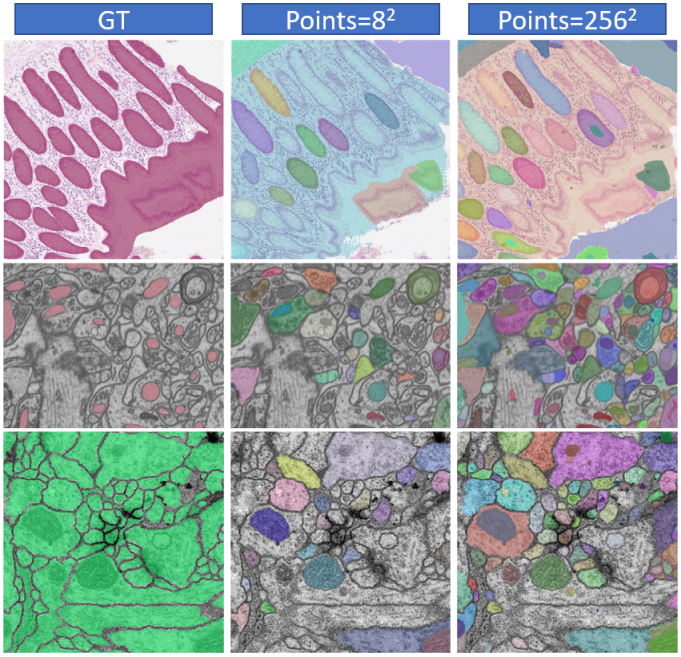
As described above, in the Everything mode, a grid of point prompts (mm) will be generated. In default, m is set to 32. The number of points will have an impact on the final segmentation performance. Especially for images that have multiple targets with different sizes, improper parameter designs will lead to imperfect segmentation with some objects being unprompted. As shown in Table 5, we tested four datasets with multiple objects on one image. The results show that in these four datasets, as the number of points increases from to , the DICE also increases gradually. Fig. 11 also shows that more points will bring more potential objects (shown in different colors). Additionally, too many points make SAM split an object into several pieces, destroying the integrity of the object. Increasing the number of points can also lead to a significant increase in test time. Hence, it is a trade-off between segmentation performance and test efficiency.

4.8 Analysis of Factors Correlating to Segmentation Results
To verify the factors that affect the segmentation performance of SAM, we recorded the size, aspect ratio, intensity difference between foreground and background, modality, and boundary complexity of 191,779 anatomical structures. By analyzing these factors, we aim to better understand the correlation between anatomical structure characteristics and SAM’s segmentation performance, and further provide some useful insights into the development of medical SAM.
The size of the anatomical structure was computed as the pixel-level area of the corresponding mask. To determine the aspect ratio of a mask, we need to calculate the ratio (ranging from 0 to 1) between the short and long sides of its bounding box. The intensity difference was defined as the variation in mean intensity values between the structure and the surrounding area within an enlarged bounding box, excluding the structure itself. Specifically, to accommodate the varied dimensions of targets, we dynamically expanded the box outward by a preset ratio of , instead of using fixed pixel values (e.g., extending by 10 pixels). Additionally, the modality of each anatomical structure was mapped to numerical values. Furthermore, we introduced Elliptical Fourier Descriptors (EFD) [51] to describe boundary complexity.
| Strategy | Size | Intensity Difference | Fourier Order | Modality | Aspect Ratio | |||||
|---|---|---|---|---|---|---|---|---|---|---|
| ViT-B | ViT-H | ViT-B | ViT-H | ViT-B | ViT-H | ViT-B | ViT-H | ViT-B | ViT-H | |
| 0.218 | 0.271 | 0.503 | 0.614 | -0.419 | -0.453 | -0.006 | 0.048 | 0.056 | 0.035 | |
| 0.236 | 0.293 | 0.572 | 0.535 | -0.537 | -0.519 | 0.051 | 0.049 | 0.079 | 0.072 | |
| 0.289 | 0.330 | 0.638 | 0.591 | -0.520 | -0.537 | 0.094 | 0.065 | 0.046 | 0.053 | |
| 0.275 | 0.339 | 0.628 | 0.533 | -0.524 | -0.533 | 0.062 | 0.040 | 0.048 | 0.060 | |
| 0.410 | 0.428 | 0.445 | 0.407 | -0.479 | -0.463 | -0.023 | -0.034 | 0.065 | 0.076 | |
| 0.370 | 0.392 | 0.467 | 0.412 | -0.621 | -0.576 | 0.014 | -0.011 | 0.068 | 0.071 | |

EFD encodes the contour of a mask into a Fourier series that represents different frequency components. As the Fourier order (FO) increases, the contour decoded from the Fourier series gets closer to the original contour (see Fig. 12), and the decoding process can be described as Eq. 2.
| (2) |
where is the coordinates of any point on the contour, is the number of Fourier series expansions, and denotes the different sampling locations. indicates the coordinates of the contour’s center point, denotes the parameter obtained by Fourier coding of the x-coordinates, and denotes the encoding result in the y-direction. We can roughly estimate the complexity of the object boundary in terms of the FO. Specifically, the order is defined as the required number of accumulations when the contour from the decoded Fourier series reaches a certain degree of overlap (we use DICE to represent overlap) with the original contour. However, when using this approach as a quantitative measure, it is especially important to set an appropriate DICE threshold.
A low threshold cannot accurately distinguish the difference in complexity among various object boundaries. If the threshold is too high, the EFD may fail to fit the complex contours as required and get into an infinite calculation. Thus, we optimized the representation of FO to avoid the EFD program from getting stuck in endless accumulation (see cumulative terms in Eq. 2).
For different structures, we increased the FO from 1 and calculated the DICE between the decoded contour and the original contour at each step. Then we set two ways to end the process: 1) ; 2) the difference in the DICE between order and order is less than . Consequently, we record the FO () and DICE after termination. Finally, we take as the final optimized FO.

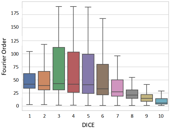
We conducted an analysis of the partial correlation between the five attributes of the target objects mentioned above and the DICE score using Spearman’s rank partial correlation coefficient under different testing strategies. The statistical results are displayed in Table 6, while Fig. 13 illustrates the scatterplot for the strategies. Across most testing strategies, we observed that the DICE score exhibited a moderate correlation () with the FO and intensity difference, a weak correlation () with the size, and no correlation with the modality and aspect ratio. Thus, SAM can consistently segment medical targets with different modality and aspect ratios. The performance of SAM under box prompt might be affected by the size of anatomical structures. Furthermore, the performance of SAM tends to be poor under all testing strategies when dealing with objects characterized by complex boundaries or low contrast. To confirm these findings, we divided DICE calculated under into ten levels on average (e.g., level-1 means DICE (%) belongs to (0,10]) and visualized the FO boxplot for different DICE levels in Fig. 14. The figure illustrates that as the DICE level increases, the FO distribution of the structures gradually shifts to a range with smaller values. Additionally, in Fig. 15, we presented visualizations of anatomical structures with various FO ranges. These visualizations reveal that the DICE score of anatomical structures tends to decrease as the FO increases. It further implies that shape and boundary complexity may have an impact on SAM’s segmentation performance.
4.9 Annotation Time and Quality Analysis
In this section, we discuss whether the SAM can help doctors improve annotation time and quality. We randomly sampled 100 images with average DICE performance from COSMOS 1050K, to construct an evaluation subset comprising 55 objects and 620 masks across 9 modalities, including instances of the same object in different modalities. We then invited three doctors with 10 years of experience to evaluate whether SAM’s prediction under box prompts could improve annotation speed and quality. They were given tasks including 1) annotating all objects in the evaluation subset from scratch, 2) adjusting object labels based on SAM’s predictions, and 3) recording the time for both tasks. To evaluate annotation quality, we utilize the Human Correction Efforts (HCE) index [83], which estimates the human effort required to correct inaccurate predictions to meet specific accuracy (i.e., GT masks) requirements in real-world applications. The lower HCE index represents that the mask (annotation of human with/without SAM) is closer to GT, i.e., annotation is of higher quality. As shown in Table 7, with SAM’s help, it can attain higher annotation quality (HCE: 0.27) and boost annotation speed by approximately 25%. Specifically, 1.31 minutes can be saved for annotating one image, and 0.2 minutes for one object (since one image contains 6.2 objects in the above task). The greater the number of anatomical structures that need to be labeled, the more obvious the advantage of SAM’s efficiency will be.
| SAM | Doctor | Human | Human with SAM | |||
|---|---|---|---|---|---|---|
| HCE | Time (s) | HCE | Time (m) | HCE | Time (m) | |
| 5.66 | 0.47 | Doctor1 | 4.74 | 4.41 | 4.57 | 3.03 |
| Doctor2 | 5.82 | 4.21 | 5.23 | 2.95 | ||
| Doctor3 | 4.65 | 4.19 | 4.59 | 2.91 | ||
| Mean | 5.07 | 4.27 | 4.80 | 2.96 | ||
4.10 Impact of Different Prompt Randomness on Performance
In the previous experiments, we fixed the box and point selection strategy for the repeatability of the experiments. We tested the theoretical optimum performance of SAM via the selection of the center of mass and tight box because they may include the most representative features of the target. However, it is not practical to click the exact center or draw the exact box of each object to evaluate SAM. Thus, we added different levels of randomness to the centers and boxes to simulate real-life human operation [35]. Besides, we believe that this can help us better discuss the robustness of SAM.
Specifically, we enlarge/move the boxes/points randomly in 0-10, 10-20, and 20-30 pixels. In Table 8, the random experiments (Random 1-3) were conducted three times, and the average results were calculated (Mean). DICE drop represents the average declining DICE value compared to the original results without shifting. For (single point), the DICE performance dropped by 2.67%, 7.38%, and 14.62% as the shifting level increased. With the increase in the number of point prompts ( and ), the decline of DICE could be alleviated, and the stability of the model could be improved. SAM was severely affected by box offsets (, 24.11% decrease in performance for shifts of 20-30 pixels), while this impact was even more pronounced when adding one point to the box (, with a decrease of 29.93%).
| Shift | DICE drop | |||||
|---|---|---|---|---|---|---|
| Random 1 | 0-10 | 2.74 | 0.87 | 0.79 | 3.08 | 4.57 |
| 10-20 | 7.55 | 1.42 | 1.37 | 10.24 | 13.98 | |
| 20-30 | 14.36 | 4.67 | 3.29 | 23.88 | 29.72 | |
| Random 2 | 0-10 | 2.68 | 0.90 | 0.84 | 3.24 | 4.49 |
| 10-20 | 7.42 | 1.38 | 1.29 | 10.39 | 13.83 | |
| 20-30 | 14.51 | 4.49 | 3.17 | 23.71 | 29.50 | |
| Random 3 | 0-10 | 2.60 | 0.81 | 0.73 | 3.43 | 5.02 |
| 10-20 | 7.17 | 1.19 | 1.22 | 10.87 | 14.28 | |
| 20-30 | 14.98 | 4.15 | 3.05 | 24.73 | 30.58 | |
| Mean | 0-10 | 2.67 | 0.86 | 0.79 | 3.25 | 4.69 |
| 10-20 | 7.38 | 1.33 | 1.29 | 10.50 | 14.03 | |
| 20-30 | 14.62 | 4.44 | 3.17 | 24.11 | 29.93 | |


4.11 Comparison between SAM and Interactive Methods
In the previous sections, we input all the prompts to the SAM’s prompt encoder once for a fair comparison of its one-round performance. To mimic the real-life interactive segmentation procedures, we performed multi-round SAM. The point selection strategy is similar to the common interactive methods. Specifically, SAM first clicks on the center of the target, then the remaining clicks are based on false negative (FN) and false positive (FP) regions. We then compared SAM with two different strong interaction segmentation approaches, i.e., FocalClick [14] and SimpleClick [63]. Both of them are pretrained on the same number of images as SAM was.
We selected 10 typical organs/tumors, covering various modalities, shapes, sizes, and intensity distributions. Experimental results are shown in Fig. 16. Based on the DICE results, our conclusion is that: 1) SAM outperformed FocalClick and SimpleClick in the first interaction with a single point; 2) As iterations progressed, SAM’s performance increased slowly, or even declined, while the performance of the interactive method could be improved steadily; 3) Using 10 points, SAM performed worse than the interactive methods. Similar results can be found in the recently published MedIA paper [73]. We consider that the current SAM’s point-based multi-round iteration capability is weak on medical images. Future work should optimize iterative training strategies when training SAM or finetune it to enhance its ability to iterate multiple rounds [15].
4.12 Task-specific Refinement for SAM
SAM’s weak ability perception on most medical images/tasks is mainly due to the lack of training data. The training dataset of SAM, i.e., SA-1B777https://ai.meta.com/datasets/segment-anything/ contains 11 million photos, including natural locations, objects, and scenes, but without any medical images. Natural images are commonly different from medical images because they have color-encoding, relatively clear definitions and boundaries of objects, easier-to-distinguish foreground (objects) and background (non-objects), and relatively balanced size. However, most medical images are gray-scale, with unclear and complex object boundaries, similar back- and fore-ground, and wide-range image size (especially containing some very small objects).
Thus, we finetuned SAM using part of the COSMOS 1050K to improve SAM’s perception of medical objects. Specifically, we considered 45 common and typical objects for finetuning the SAM. Inspired by Ma and Wang [69], we only considered finetuning the SAM using box prompts. We fixed the image encoder to minimize computation costs and also kept the prompt encoder frozen because of its powerful capacity for encoding box positional information. Thus, only the parameters in the mask decoder were adjusted during finetuning. We set the total epoch as 20, and the learning rate and batch size are 1e-4 and 2.
The results demonstrate a general improvement in segmentation performance after finetuning for both ViT-B and ViT-H models, as shown in Fig. 17 and Fig. 18. Fig. 17 illustrates a shift towards higher DICE values across different correlating factors, indicating improved overall performance. Specifically, for ViT-B, 32 out of 45 objects exhibit performance enhancement, while ViT-H shows improvement in 37 out of 45 objects. This can prove the strong learning ability of ViT-H, because it has almost 7 times the parameters as ViT-B (636M vs. 91M). The performance of objects with small numbers, RGB color coding, etc., decreases. This reminds us that we may need to make more careful designs for task-specific finetuning. We will release all the finetuned models and source codes.
5 Conclusion
In this study, we comprehensively evaluated the SAM for the segmentation of a large medical image dataset. Based on the aforementioned empirical analyses, our conclusions are as follows: 1) SAM showed remarkable performance in some specific objects but was unstable, imperfect, or even totally failed in other situations. 2) SAM with the large ViT-H showed better overall performance than that with the small ViT-B. 3) SAM performed better with manual hints, especially box, than the Everything mode. 4) SAM could help human annotation with high labeling quality and less time. 5) SAM is sensitive to the randomness in the center point and tight box prompts, and may suffer from a serious performance drop. 6) SAM performed better than interactive methods with one or a few points, but will be outpaced as the number of points increases. 7) SAM’s performance correlated to different factors, including boundary complexity, etc. 8) Finetuning the SAM on specific medical tasks could improve its average DICE performance by 4.39% and 6.68% for ViT-B and ViT-H, respectively. Finally, we believe that, although SAM has the potential to become a general MIS model, its performance in the MIS task is not stable at present. We hope that this report will help readers and the community better understand SAM’s segmentation performance in medical images and ultimately facilitate the development of a new generation of MIS foundation models.
6 Discussion
We will focus on discussing the potential future directions of SAM, and we hope these can inspire the readers to some extent.
How is semantics obtained from SAM when there is no GT? The current SAM only has the ability to perceive objects but cannot analyze specific categories of objects. Recently, several studies have explored to address this problem, and one of them equipped the SAM with a CLIP model888https://github.com/Curt-Park/segment-anything-with-clip. Specifically, SAM will first provide the region proposals, and the region patch will be cropped from the original image. Then, the cropped patch will be input to CLIP for object classification. Another solution is to combine the SAM with an Open-Vocabulary Object Detection (OVOD) model, e.g., Grounding DINO with SAM (Grounded-SAM999https://github.com/IDEA-Research/Grounded-Segment-Anything). In this pipeline, the OVOD model can detect the bounding boxes of objects with classification results. Then, SAM will take the box region as input and output the segmentation result. Recently, semantic-SAM has been proposed to segment and recognize anything in natural images [58]. All the previous explorations are based on natural images. Thus, it may be interesting to develop medical SAM with semantic awareness. However, it is challenging because medical objects in the open scene have varied and complex shapes, a wide variety of types, and many similar subclasses (tumors of different grades, etc.).
SAM vs. traditional segmentation methods? Finetuning SAM with limited medical data can outperform task-specific traditional segmentation methods. This has been validated in several recently published studies. Med-SAM has proven that finetuning the 2D SAM can achieve superior performance to specialist Unet models in most cases [69]. 3D modality-agnostic SAM (MA-SAM) has validated that finetuning SAM with 3D adapters can outperform traditional SOTA 3D nn-Unet, even without any prompts [13]. It also sheds some light on the medical image segmentation community, suggesting that perhaps finetuning the fundamental segmentation model will perform better than training a traditional segmentation model from scratch. However, there are still some problems with SAM, including model robustness to different prompt noises and multi-round interaction ability.
2D or 3D SAM? For medical data, variability in imaging modalities (2D/videos/3D/4D) may make the design of general models complex. Compared to videos/3D/4D images (CT/MRI, etc.), 2D is more foundational and common in medical data. Thus, it is more practical to build a 2D model that can process all types of data consistently, as video/3D/4D data can be transferred to a series of 2D slices [69]. The limited amount of 3D data (SAM: 11M images and 1B masks vs. Ours: 10K volumes and 45K masks) may restrict the construction of 3D fundamental segmentation models, especially if training from scratch is required. To break the limitation of data, we will explore how to synthesize more high-fidelity 3D data and build a strong fundamental model for medical image segmentation.
SAM boosts large-scale medical annotation? Developing robust and effective deep learning-based medical segmentation models highly requires large-scale and fully-labeled datasets. This is very challenging for current schemes based on manual annotation by experts. As introduced in [84], annotating 8,448 CT volumes with 9 anatomical structures and 3.2 million slices requires roughly 30.8 years for one experienced expert. They shorten the annotation time to three weeks with the help of multiple pre-trained segmentation models for generating pseudo labels, and other useful strategies. However, obtaining well-performing pre-trained models, especially with low false positives, is still very difficult. Moreover, segmentation networks based on traditional deep learning cannot well support human-computer interaction, limiting its flexibility. The occurrence of SAM with promptable segmentation brings hope to solve the challenges. Our study also preliminarily verified that SAM can greatly shorten the annotation time and improve the annotation quality. The greater the number of anatomical structures that need to be labeled, the more obvious the advantage of SAM’s efficiency will be. Notably, the design of the SAM paradigm has the potential to achieve universal segmentation. It means that a single SAM network can be used to achieve the annotation of large-scale multi-modal, multi-class medical datasets, rather than using multiple task-specific models. This is important for lightweight and efficient deployment of models in labeling software, e.g., MONAI Label [12] and Pair annotation software package [60].
7 Acknowledgement
The authors of this paper sincerely appreciate all the challenge organizers and owners for providing the public MIS datasets including AbdomenCT-1K, ACDC, AMOS 2022, AutoLaparo, BrainPTM 2021, BraTS20, CAMUS, CHAOS, CHASE-DB1, Chest CT segmentation, CRAG, crossMoDA, CVC-ClinicDB, DRIVE, EndoTect 2020, EPFL-EM, ETIS-Larib Polyp DB, FeTA, HaN-Seg, I2CVB, iChallenge-AMD, iChallenge-PALM, IDRiD 2018, iSeg 2019, ISIC 2018, IXI, KiPA22, KiTS19, KiTS21, Kvasir-Instrumen, Kvasir-SEG, iVScar, LUNA16, M&Ms, MALBCV-Abdomen, Montgomery County CXR Set, MRSpineSeg, MSD, NCI-ISBI 2013, CellSeg Challenge-NeurIPS 2022, PROMISE12, QUBIQ 2021, SIIM-ACR, SKI10, SLIVER07, ssTEM, STARE, TN-SCUI, TotalSegmentator, VerSe19VerSe20, Warwick-QU, WORD, and 4C2021 C04 TLS01. We also thank Meta AI for releasing the source code of SAM publicly available.
This work was supported by the grant from National Natural Science Foundation of China (Nos. 62171290, 62101343), Shenzhen-Hong Kong Joint Research Program (No. SGDX20201103095613036), and Shenzhen Science and Technology Innovations Committee (No. 20200812143441001).
8 Supplementary materials
Comprehensive quantitative and qualitative results can be found at https://github.com/yuhoo0302/Segment-Anything-Model-for-Medical-Images/blob/main/Supplementary_Materials.pdf.
References
- Antonelli et al. [2022] Antonelli, M., Reinke, A., Bakas, S., Farahani, K., Kopp-Schneider, A., Landman, B.A., Litjens, G., Menze, B., Ronneberger, O., Summers, R.M., et al., 2022. The medical segmentation decathlon. Nature communications 13, 4128.
- Avital et al. [2019] Avital, I., Nelkenbaum, I., Tsarfaty, G., Konen, E., Kiryati, N., Mayer, A., 2019. Neural segmentation of seeding rois (srois) for pre-surgical brain tractography. IEEE transactions on medical imaging 39, 1655–1667.
- Bakas et al. [2017] Bakas, S., Akbari, H., Sotiras, A., Bilello, M., Rozycki, M., Kirby, J.S., Freymann, J.B., Farahani, K., Davatzikos, C., 2017. Advancing the cancer genome atlas glioma mri collections with expert segmentation labels and radiomic features. Scientific data 4, 1–13.
- Bakas et al. [2018] Bakas, S., Reyes, M., Jakab, A., Bauer, S., Rempfler, M., Crimi, A., Shinohara, R.T., Berger, C., Ha, S.M., Rozycki, M., et al., 2018. Identifying the best machine learning algorithms for brain tumor segmentation, progression assessment, and overall survival prediction in the brats challenge. arXiv preprint arXiv:1811.02629 .
- Bernal et al. [2015] Bernal, J., Sánchez, F.J., Fernández-Esparrach, G., Gil, D., Rodríguez, C., Vilariño, F., 2015. Wm-dova maps for accurate polyp highlighting in colonoscopy: Validation vs. saliency maps from physicians. Computerized medical imaging and graphics 43, 99–111.
- Bernal et al. [2017] Bernal, J., Tajkbaksh, N., Sanchez, F.J., Matuszewski, B.J., Chen, H., Yu, L., Angermann, Q., Romain, O., Rustad, B., Balasingham, I., et al., 2017. Comparative validation of polyp detection methods in video colonoscopy: results from the miccai 2015 endoscopic vision challenge. IEEE transactions on medical imaging 36, 1231–1249.
- Bernard et al. [2018] Bernard, O., Lalande, A., Zotti, C., Cervenansky, F., Yang, X., Heng, P.A., Cetin, I., Lekadir, K., Camara, O., Ballester, M.A.G., et al., 2018. Deep learning techniques for automatic mri cardiac multi-structures segmentation and diagnosis: is the problem solved? IEEE transactions on medical imaging 37, 2514–2525.
- Bilic et al. [2023] Bilic, P., Christ, P., Li, H.B., Vorontsov, E., Ben-Cohen, A., Kaissis, G., Szeskin, A., Jacobs, C., Mamani, G.E.H., Chartrand, G., et al., 2023. The liver tumor segmentation benchmark (lits). Medical Image Analysis 84, 102680.
- Butoi* et al. [2023] Butoi*, V.I., Ortiz*, J.J.G., Ma, T., Sabuncu, M.R., Guttag, J., Dalca, A.V., 2023. Universeg: Universal medical image segmentation. International Conference on Computer Vision .
- Campello et al. [2021] Campello, V.M., Gkontra, P., Izquierdo, C., Martin-Isla, C., Sojoudi, A., Full, P.M., Maier-Hein, K., Zhang, Y., He, Z., Ma, J., et al., 2021. Multi-centre, multi-vendor and multi-disease cardiac segmentation: the m&ms challenge. IEEE Transactions on Medical Imaging 40, 3543–3554.
- Cardona et al. [2010] Cardona, A., Saalfeld, S., Preibisch, S., Schmid, B., Cheng, A., Pulokas, J., Tomancak, P., Hartenstein, V., 2010. An integrated micro-and macroarchitectural analysis of the drosophila brain by computer-assisted serial section electron microscopy. PLoS biology 8, e1000502.
- Cardoso et al. [2022] Cardoso, M.J., Li, W., Brown, R., Ma, N., Kerfoot, E., Wang, Y., Murrey, B., Myronenko, A., Zhao, C., et al., 2022. Monai: An open-source framework for deep learning in healthcare. arXiv preprint arXiv:2211.02701 .
- Chen et al. [2023] Chen, C., Miao, J., Wu, D., Yan, Z., Kim, S., Hu, J., Zhong, A., Liu, Z., Sun, L., Li, X., Liu, T., Heng, P.A., Li, Q., 2023. Ma-sam: Modality-agnostic sam adaptation for 3d medical image segmentation. arXiv:2309.08842.
- Chen et al. [2022] Chen, X., Zhao, Z., Zhang, Y., Duan, M., Qi, D., Zhao, H., 2022. Focalclick: Towards practical interactive image segmentation, in: Proceedings of the IEEE/CVF Conference on Computer Vision and Pattern Recognition, pp. 1300--1309.
- Cheng et al. [2023] Cheng, J., Ye, J., Deng, Z., Chen, J., Li, T., Wang, H., Su, Y., Huang, Z., Chen, J., Jiang, L., et al., 2023. Sam-med2d. arXiv preprint arXiv:2308.16184 .
- Codella et al. [2019] Codella, N., Rotemberg, V., Tschandl, P., Celebi, M.E., Dusza, S., Gutman, D., Helba, B., Kalloo, A., Liopyris, K., et al., 2019. Skin lesion analysis toward melanoma detection 2018: A challenge hosted by the international skin imaging collaboration (isic). arXiv preprint arXiv:1902.03368 .
- Codella et al. [2018] Codella, N.C., Gutman, D., Celebi, M.E., Helba, B., Marchetti, M.A., Dusza, S.W., Kalloo, A., Liopyris, K., Mishra, N., Kittler, H., et al., 2018. Skin lesion analysis toward melanoma detection: A challenge at the 2017 international symposium on biomedical imaging (isbi), hosted by the international skin imaging collaboration (isic), in: 2018 IEEE 15th international symposium on biomedical imaging (ISBI 2018), IEEE. pp. 168--172.
- Crum et al. [2006] Crum, W.R., Camara, O., Hill, D.L., 2006. Generalized overlap measures for evaluation and validation in medical image analysis. IEEE transactions on medical imaging 25, 1451--1461.
- Dataset [a] Dataset, C.C.S., a. Chest CT Segmentation Dataset. [EB/OL]. https://www.kaggle.com/datasets/polomarco/chest-ct-segmentation.
- Dataset [b] Dataset, C.C.T., b. 4c2021 c04 tls01 dataset. [EB/OL]. https://aistudio.baidu.com/aistudio/projectdetail/1952488?channelType=1&channel=1.
- Dataset [c] Dataset, I., c. IXI Dataset. [EB/OL]. https://brain-development.org/ixi-dataset/.
- Deng et al. [2023] Deng, R., Cui, C., Liu, Q., Yao, T., Remedios, L.W., Bao, S., Landman, B.A., Tang, Y., Wheless, L.E., Coburn, L.A., et al., 2023. Segment anything model (sam) for digital pathology: Assess zero-shot segmentation on whole slide imaging, in: Medical Imaging with Deep Learning, short paper track.
- Dice [1945] Dice, L.R., 1945. Measures of the amount of ecologic association between species. Ecology 26, 297--302.
- Dosovitskiy et al. [2020] Dosovitskiy, A., Beyer, L., Kolesnikov, A., Weissenborn, D., Zhai, X., Unterthiner, T., Dehghani, M., Minderer, M., Heigold, G., Gelly, S., et al., 2020. An image is worth 16x16 words: Transformers for image recognition at scale, in: International Conference on Learning Representations.
- Graham et al. [2019] Graham, S., Chen, H., Gamper, J., Dou, Q., Heng, P.A., Snead, D., Tsang, Y.W., Rajpoot, N., 2019. Mild-net: Minimal information loss dilated network for gland instance segmentation in colon histology images. Medical image analysis 52, 199--211.
- He et al. [2022] He, K., Chen, X., Xie, S., Li, Y., Dollár, P., Girshick, R., 2022. Masked autoencoders are scalable vision learners, in: Proceedings of the IEEE/CVF Conference on Computer Vision and Pattern Recognition, pp. 16000--16009.
- He et al. [2023] He, S., Bao, R., Li, J., Grant, P.E., Ou, Y., 2023. Accuracy of segment-anything model (sam) in medical image segmentation tasks. arXiv preprint arXiv:2304.09324 .
- He et al. [2020] He, Y., Yang, G., Yang, J., Chen, Y., Kong, Y., Wu, J., Tang, L., Zhu, X., Dillenseger, J.L., Shao, P., et al., 2020. Dense biased networks with deep priori anatomy and hard region adaptation: Semi-supervised learning for fine renal artery segmentation. Medical image analysis 63, 101722.
- He et al. [2021] He, Y., Yang, G., Yang, J., Ge, R., Kong, Y., Zhu, X., Zhang, S., Shao, P., Shu, H., Dillenseger, J.L., et al., 2021. Meta grayscale adaptive network for 3d integrated renal structures segmentation. Medical image analysis 71, 102055.
- Heimann et al. [2009] Heimann, T., Van Ginneken, B., Styner, M.A., Arzhaeva, Y., Aurich, V., Bauer, C., Beck, A., Becker, C., Beichel, R., Bekes, G., et al., 2009. Comparison and evaluation of methods for liver segmentation from ct datasets. IEEE transactions on medical imaging 28, 1251--1265.
- Heller et al. [2020] Heller, N., Sathianathen, N., Kalapara, A., Walczak, E., Moore, K., Kaluzniak, H., Rosenberg, J., Blake, P., Rengel, Z., Oestreich, M., Dean, J., Tradewell, M., Shah, A., Tejpaul, R., Edgerton, Z., Peterson, M., Raza, S., Regmi, S., Papanikolopoulos, N., Weight, C., 2020. The kits19 challenge data: 300 kidney tumor cases with clinical context, ct semantic segmentations, and surgical outcomes. arXiv:1904.00445.
- Hicks et al. [2021] Hicks, S.A., Jha, D., Thambawita, V., Halvorsen, P., Hammer, H.L., Riegler, M.A., 2021. The endotect 2020 challenge: evaluation and comparison of classification, segmentation and inference time for endoscopy, in: Pattern Recognition. ICPR International Workshops and Challenges: Virtual Event, January 10-15, 2021, Proceedings, Part VIII, Springer. pp. 263--274.
- Hoover and Goldbaum [2003] Hoover, A., Goldbaum, M., 2003. Locating the optic nerve in a retinal image using the fuzzy convergence of the blood vessels. IEEE transactions on medical imaging 22, 951--958.
- Hoover et al. [2000] Hoover, A., Kouznetsova, V., Goldbaum, M., 2000. Locating blood vessels in retinal images by piecewise threshold probing of a matched filter response. IEEE Transactions on Medical imaging 19, 203--210.
- Huang et al. [2021] Huang, Y., Yang, X., Zou, Y., Chen, C., Wang, J., Dou, H., Ravikumar, N., Frangi, A.F., Zhou, J., Ni, D., 2021. Flip learning: Erase to segment, in: Medical Image Computing and Computer Assisted Intervention--MICCAI 2021: 24th International Conference, Strasbourg, France, September 27--October 1, 2021, Proceedings, Part I 24, Springer. pp. 493--502.
- Huazhu et al. [2019] Huazhu, F., Fei, L., José, I., 2019. Palm: Pathologic myopia challenge. Comput. Vis. Med. Imaging .
- Isensee et al. [2021] Isensee, F., Jaeger, P.F., Kohl, S.A., Petersen, J., Maier-Hein, K.H., 2021. nnu-net: a self-configuring method for deep learning-based biomedical image segmentation. Nature methods 18, 203--211.
- Jaccard [1908] Jaccard, P., 1908. Nouvelles recherches sur la distribution florale. Bull. Soc. Vaud. Sci. Nat. 44, 223--270.
- Jaeger et al. [2014] Jaeger, S., Candemir, S., Antani, S., Wáng, Y.X.J., Lu, P.X., Thoma, G., 2014. Two public chest x-ray datasets for computer-aided screening of pulmonary diseases. Quantitative imaging in medicine and surgery 4, 475.
- Jha et al. [2021] Jha, D., Ali, S., Emanuelsen, K., Hicks, S.A., Thambawita, V., Garcia-Ceja, E., Riegler, M.A., de Lange, T., Schmidt, P.T., Johansen, H.D., Johansen, D., Halvorsen, P., 2021. Kvasir-instrument: Diagnostic and therapeutic tool segmentation dataset in gastrointestinal endoscopy, in: MultiMedia Modeling, Springer International Publishing, Cham. pp. 218--229.
- Jha et al. [2020] Jha, D., Smedsrud, P.H., Riegler, M.A., Halvorsen, P., de Lange, T., Johansen, D., Johansen, H.D., 2020. Kvasir-seg: A segmented polyp dataset, in: International Conference on Multimedia Modeling, Springer. pp. 451--462.
- Ji et al. [2023a] Ji, G.P., Fan, D.P., Xu, P., Cheng, M.M., Zhou, B., Van Gool, L., 2023a. Sam struggles in concealed scenes--empirical study on" segment anything". SCIENCE CHINA Information Sciences (SCIS) .
- Ji et al. [2023b] Ji, W., Li, J., Bi, Q., Li, W., Cheng, L., 2023b. Segment anything is not always perfect: An investigation of sam on different real-world applications. arXiv preprint arXiv:2304.05750 .
- Ji et al. [2021] Ji, W., Yu, S., Wu, J., Ma, K., Bian, C., Bi, Q., Li, J., Liu, H., Cheng, L., Zheng, Y., 2021. Learning calibrated medical image segmentation via multi-rater agreement modeling, in: Proceedings of the IEEE/CVF Conference on Computer Vision and Pattern Recognition, pp. 12341--12351.
- Ji et al. [2022] Ji, Y., Bai, H., Yang, J., Luo, P., 2022. Amos: A large-scale abdominal multi-organ benchmark for versatile medical image segmentation. Advances In Neural Information Processing Systems (NeurlPS) Benchmark and Dataset Track .
- Jia et al. [2021] Jia, C., Yang, Y., Xia, Y., Chen, Y.T., Parekh, Z., Pham, H., Le, Q., Sung, Y.H., Li, Z., Duerig, T., 2021. Scaling up visual and vision-language representation learning with noisy text supervision, in: International Conference on Machine Learning, PMLR. pp. 4904--4916.
- Karim et al. [2016] Karim, R., Bhagirath, P., Claus, P., Housden, R.J., Chen, Z., Karimaghaloo, Z., Sohn, H.M., Rodríguez, L.L., Vera, S., Albà, X., et al., 2016. Evaluation of state-of-the-art segmentation algorithms for left ventricle infarct from late gadolinium enhancement mr images. Medical image analysis 30, 95--107.
- Karimi and Salcudean [2020] Karimi, D., Salcudean, S.E., 2020. Reducing the hausdorff distance in medical image segmentation with convolutional neural networks. IEEE transactions on medical imaging 39, 499--513.
- Kavur et al. [2021] Kavur, A.E., Gezer, N.S., Barış, M., Aslan, S., Conze, P.H., Groza, V., Pham, D.D., Chatterjee, S., Ernst, P., Özkan, S., et al., 2021. Chaos challenge-combined (ct-mr) healthy abdominal organ segmentation. Medical Image Analysis 69, 101950.
- Kirillov et al. [2023] Kirillov, A., Mintun, E., Ravi, N., Mao, H., Rolland, C., Gustafson, L., Xiao, T., Whitehead, S., Berg, A.C., Lo, W.Y., Dollar, P., Girshick, R., 2023. Segment anything, in: Proceedings of the IEEE/CVF International Conference on Computer Vision (ICCV), pp. 4015--4026.
- Kuhl and Giardina [1982] Kuhl, F.P., Giardina, C.R., 1982. Elliptic fourier features of a closed contour. Computer graphics and image processing 18, 236--258.
- Landman et al. [2015] Landman, B., Xu, Z., Igelsias, J., Styner, M., Langerak, T., Klein, A., 2015. Miccai multi-atlas labeling beyond the cranial vault--workshop and challenge, in: Proc. MICCAI Multi-Atlas Labeling Beyond Cranial Vault—Workshop Challenge, p. 12.
- Leclerc et al. [2019] Leclerc, S., Smistad, E., Pedrosa, J., Østvik, A., Cervenansky, F., Espinosa, F., Espeland, T., Berg, E.A.R., Jodoin, P.M., Grenier, T., et al., 2019. Deep learning for segmentation using an open large-scale dataset in 2d echocardiography. IEEE transactions on medical imaging 38, 2198--2210.
- Lee et al. [2023] Lee, G., Kim, S., Kim, J., Yun, S.Y., 2023. Mediar: Harmony of data-centric and model-centric for multi-modality microscopy, in: Proceedings of The Cell Segmentation Challenge in Multi-modality High-Resolution Microscopy Images, PMLR. pp. 1--16.
- Lee et al. [2010] Lee, S., Shim, H., Park, S.H., Yun, I.D., Lee, S.U., 2010. Learning local shape and appearance for segmentation of knee cartilage in 3d mri, in: Medical Image Analysis for the Clinic: a Grand Challenge. In Proceedings of the 13th International Conference on Medical Image Computing and Computer Assisted Intervention (MICCAI 2010), Beijing, China, pp. 231--240.
- Lemaître et al. [2015] Lemaître, G., Martí, R., Freixenet, J., Vilanova, J.C., Walker, P.M., Meriaudeau, F., 2015. Computer-aided detection and diagnosis for prostate cancer based on mono and multi-parametric mri: a review. Computers in biology and medicine 60, 8--31.
- Li et al. [2013] Li, A., Li, C., Wang, X., Eberl, S., Feng, D.D., Fulham, M., 2013. Automated segmentation of prostate mr images using prior knowledge enhanced random walker, in: 2013 International Conference on Digital Image Computing: Techniques and Applications (DICTA), IEEE. pp. 1--7.
- Li et al. [2023] Li, F., Zhang, H., Sun, P., Zou, X., Liu, S., Yang, J., Li, C., Zhang, L., Gao, J., 2023. Semantic-sam: Segment and recognize anything at any granularity. arXiv preprint arXiv:2307.04767 .
- Li et al. [2020] Li, X., Jia, M., Islam, M.T., Yu, L., Xing, L., 2020. Self-supervised feature learning via exploiting multi-modal data for retinal disease diagnosis. IEEE Transactions on Medical Imaging 39, 4023--4033.
- Liang et al. [2022] Liang, J., Yang, X., Huang, Y., Li, H., He, S., Hu, X., Chen, Z., Xue, W., Cheng, J., Ni, D., 2022. Sketch guided and progressive growing gan for realistic and editable ultrasound image synthesis. Medical Image Analysis 79, 102461.
- Liebl et al. [2021] Liebl, H., Schinz, D., Sekuboyina, A., Malagutti, L., Löffler, M.T., Bayat, A., El Husseini, M., Tetteh, G., Grau, K., Niederreiter, E., et al., 2021. A computed tomography vertebral segmentation dataset with anatomical variations and multi-vendor scanner data. Scientific Data 8, 284.
- Litjens et al. [2014] Litjens, G., Toth, R., Van De Ven, W., Hoeks, C., Kerkstra, S., van Ginneken, B., Vincent, G., Guillard, G., Birbeck, N., Zhang, J., et al., 2014. Evaluation of prostate segmentation algorithms for mri: the promise12 challenge. Medical image analysis 18, 359--373.
- Liu et al. [2023a] Liu, Q., Xu, Z., Bertasius, G., Niethammer, M., 2023a. Simpleclick: Interactive image segmentation with simple vision transformers, in: Proceedings of the IEEE/CVF International Conference on Computer Vision (ICCV), pp. 22290--22300.
- Liu et al. [2022] Liu, W., Yang, H., Tian, T., Cao, Z., Pan, X., Xu, W., Jin, Y., Gao, F., 2022. Full-resolution network and dual-threshold iteration for retinal vessel and coronary angiograph segmentation. IEEE Journal of Biomedical and Health Informatics 26, 4623--4634.
- Liu et al. [2023b] Liu, Y., Zhang, J., She, Z., Kheradmand, A., Armand, M., 2023b. Samm (segment any medical model): A 3d slicer integration to sam. arXiv preprint arXiv:2304.05622 .
- Löffler et al. [2020] Löffler, M.T., Sekuboyina, A., Jacob, A., Grau, A.L., Scharr, A., El Husseini, M., Kallweit, M., Zimmer, C., Baum, T., Kirschke, J.S., 2020. A vertebral segmentation dataset with fracture grading. Radiology: Artificial Intelligence 2, e190138.
- Lucchi et al. [2013] Lucchi, A., Li, Y., Fua, P., 2013. Learning for structured prediction using approximate subgradient descent with working sets, in: Proceedings of the IEEE Conference on Computer Vision and Pattern Recognition, pp. 1987--1994.
- Luo et al. [2022] Luo, X., Liao, W., Xiao, J., Chen, J., Song, T., Zhang, X., Li, K., Metaxas, D.N., Wang, G., Zhang, S., 2022. Word: A large scale dataset, benchmark and clinical applicable study for abdominal organ segmentation from ct image. Medical Image Analysis 82, 102642.
- Ma and Wang [2023] Ma, J., Wang, B., 2023. Segment anything in medical images. arXiv:2304.12306.
- Ma et al. [2023] Ma, J., Xie, R., Ayyadhury, S., Ge, C., Gupta, A., Gupta, R., Gu, S., Zhang, Y., Lee, G., Kim, J., Lou, W., Li, H., Upschulte, E., Dickscheid, T., de Almeida, J.G., Wang, Y., Han, L., Yang, X., Labagnara, M., Rahi, S.J., Kempster, C., Pollitt, A., Espinosa, L., Mignot, T., Middeke, J.M., Eckardt, J.N., Li, W., Li, Z., Cai, X., Bai, B., Greenwald, N.F., Valen, D.V., Weisbart, E., Cimini, B.A., Li, Z., Zuo, C., Brück, O., Bader, G.D., Wang, B., 2023. The multi-modality cell segmentation challenge: Towards universal solutions. arXiv:2308.05864 .
- Ma et al. [2021] Ma, J., Zhang, Y., Gu, S., Zhu, C., Ge, C., Zhang, Y., An, X., Wang, C., Wang, Q., Liu, X., et al., 2021. Abdomenct-1k: Is abdominal organ segmentation a solved problem? IEEE Transactions on Pattern Analysis and Machine Intelligence 44, 6695--6714.
- Mattjie et al. [2023] Mattjie, C., Vinicius de Moura, L., Cappelari Ravazio, R., Silveira Kupssinskü, L., Parraga, O., Mussi Delucis, M., Coelho Barros, R., 2023. Exploring the zero-shot capabilities of the segment anything model (sam) in 2d medical imaging: A comprehensive evaluation and practical guideline. arXiv e-prints , arXiv--2305.
- Mazurowski et al. [2023] Mazurowski, M.A., Dong, H., Gu, H., Yang, J., Konz, N., Zhang, Y., 2023. Segment anything model for medical image analysis: an experimental study. Medical Image Analysis 89, 102918.
- Menze et al. [2014] Menze, B.H., Jakab, A., Bauer, S., Kalpathy-Cramer, J., Farahani, K., Kirby, J., Burren, Y., Porz, N., Slotboom, J., Wiest, R., et al., 2014. The multimodal brain tumor image segmentation benchmark (brats). IEEE transactions on medical imaging 34, 1993--2024.
- Mohapatra et al. [2023] Mohapatra, S., Gosai, A., Schlaug, G., 2023. Brain extraction comparing segment anything model (sam) and fsl brain extraction tool. arXiv preprint arXiv:2304.04738 .
- Nelkenbaum et al. [2020] Nelkenbaum, I., Tsarfaty, G., Kiryati, N., Konen, E., Mayer, A., 2020. Automatic segmentation of white matter tracts using multiple brain mri sequences, in: 2020 IEEE 17th International Symposium on Biomedical Imaging (ISBI), IEEE. pp. 368--371.
- Pang et al. [2020] Pang, S., Pang, C., Zhao, L., Chen, Y., Su, Z., Zhou, Y., Huang, M., Yang, W., Lu, H., Feng, Q., 2020. Spineparsenet: spine parsing for volumetric mr image by a two-stage segmentation framework with semantic image representation. IEEE Transactions on Medical Imaging 40, 262--273.
- Payette et al. [2021] Payette, K., de Dumast, P., Kebiri, H., Ezhov, I., Paetzold, J.C., Shit, S., Iqbal, A., Khan, R., Kottke, R., Grehten, P., et al., 2021. An automatic multi-tissue human fetal brain segmentation benchmark using the fetal tissue annotation dataset. Scientific Data 8, 167.
- Pieper et al. [2004] Pieper, S., Halle, M., Kikinis, R., 2004. 3d slicer, in: 2004 2nd IEEE international symposium on biomedical imaging: nano to macro (IEEE Cat No. 04EX821), IEEE. pp. 632--635.
- Podobnik et al. [2023] Podobnik, G., Strojan, P., Peterlin, P., Ibragimov, B., Vrtovec, T., 2023. Han-seg: The head and neck organ-at-risk ct & mr segmentation dataset. Medical Physics .
- Porwal et al. [2018] Porwal, P., Pachade, S., Kamble, R., Kokare, M., Deshmukh, G., Sahasrabuddhe, V., Meriaudeau, F., 2018. Indian diabetic retinopathy image dataset (idrid): a database for diabetic retinopathy screening research. Data 3, 25.
- Qian et al. [2022] Qian, J., Li, R., Yang, X., Huang, Y., Luo, M., Lin, Z., Hong, W., Huang, R., Fan, H., Ni, D., et al., 2022. Hasa: hybrid architecture search with aggregation strategy for echinococcosis classification and ovary segmentation in ultrasound images. Expert Systems with Applications 202, 117242.
- Qin et al. [2022] Qin, X., Dai, H., Hu, X., Fan, D.P., Shao, L., Van Gool, L., 2022. Highly accurate dichotomous image segmentation, in: European Conference on Computer Vision, Springer. pp. 38--56.
- Qu et al. [2023] Qu, C., Zhang, T., Qiao, H., Liu, J., Tang, Y., Yuille, A., Zhou, Z., 2023. Abdomenatlas-8k: Annotating 8,000 CT volumes for multi-organ segmentation in three weeks, in: Thirty-seventh Conference on Neural Information Processing Systems Datasets and Benchmarks Track.
- Radford et al. [2021] Radford, A., Kim, J.W., Hallacy, C., Ramesh, A., Goh, G., Agarwal, S., Sastry, G., Askell, A., Mishkin, P., Clark, J., et al., 2021. Learning transferable visual models from natural language supervision, in: International conference on machine learning, PMLR. pp. 8748--8763.
- Ramesh et al. [2021] Ramesh, A., Pavlov, M., Goh, G., Gray, S., Voss, C., Radford, A., Chen, M., Sutskever, I., 2021. Zero-shot text-to-image generation, in: International Conference on Machine Learning, PMLR. pp. 8821--8831.
- Sekuboyina et al. [2021] Sekuboyina, A., Husseini, M.E., Bayat, A., Löffler, M., Liebl, H., Li, H., Tetteh, G., Kukačka, J., Payer, C., Štern, D., et al., 2021. Verse: A vertebrae labelling and segmentation benchmark for multi-detector ct images. Medical image analysis 73, 102166.
- Setio et al. [2017] Setio, A.A.A., Traverso, A., De Bel, T., Berens, M.S., Van Den Bogaard, C., Cerello, P., Chen, H., Dou, Q., Fantacci, M.E., Geurts, B., et al., 2017. Validation, comparison, and combination of algorithms for automatic detection of pulmonary nodules in computed tomography images: the luna16 challenge. Medical image analysis 42, 1--13.
- Shao et al. [2011] Shao, P., Qin, C., Yin, C., Meng, X., Ju, X., Li, J., Lv, Q., Zhang, W., Xu, Z., 2011. Laparoscopic partial nephrectomy with segmental renal artery clamping: technique and clinical outcomes. European urology 59, 849--855.
- Shao et al. [2012] Shao, P., Tang, L., Li, P., Xu, Y., Qin, C., Cao, Q., Ju, X., Meng, X., Lv, Q., Li, J., et al., 2012. Precise segmental renal artery clamping under the guidance of dual-source computed tomography angiography during laparoscopic partial nephrectomy. European urology 62, 1001--1008.
- Shapey et al. [2021] Shapey, J., Kujawa, A., Dorent, R., Wang, G., Bisdas, S., Dimitriadis, A., Grishchuck, D., Paddick, I., Kitchen, N., Bradford, R., et al., 2021. Segmentation of vestibular schwannoma from magnetic resonance imaging: An open annotated dataset and baseline algorithm (vestibular-schwannoma-seg).
- Shapey et al. [2019] Shapey, J., Wang, G., Dorent, R., Dimitriadis, A., Li, W., Paddick, I., Kitchen, N., Bisdas, S., Saeed, S.R., Ourselin, S., et al., 2019. An artificial intelligence framework for automatic segmentation and volumetry of vestibular schwannomas from contrast-enhanced t1-weighted and high-resolution t2-weighted mri. Journal of neurosurgery 134, 171--179.
- Simpson et al. [2019] Simpson, A.L., Antonelli, M., Bakas, S., Bilello, M., Farahani, K., Van Ginneken, B., Kopp-Schneider, A., Landman, B.A., Litjens, G., Menze, B., et al., 2019. A large annotated medical image dataset for the development and evaluation of segmentation algorithms. arXiv preprint arXiv:1902.09063 .
- Sirinukunwattana et al. [2017] Sirinukunwattana, K., Pluim, J.P., Chen, H., Qi, X., Heng, P.A., Guo, Y.B., Wang, L.Y., Matuszewski, B.J., Bruni, E., Sanchez, U., et al., 2017. Gland segmentation in colon histology images: The glas challenge contest. Medical image analysis 35, 489--502.
- Sun et al. [2021] Sun, Y., Gao, K., Wu, Z., Li, G., Zong, X., Lei, Z., Wei, Y., Ma, J., Yang, X., Feng, X., et al., 2021. Multi-site infant brain segmentation algorithms: the iseg-2019 challenge. IEEE Transactions on Medical Imaging 40, 1363--1376.
- Tancik et al. [2020] Tancik, M., Srinivasan, P., Mildenhall, B., Fridovich-Keil, S., Raghavan, N., Singhal, U., Ramamoorthi, R., Barron, J., Ng, R., 2020. Fourier features let networks learn high frequency functions in low dimensional domains. Advances in Neural Information Processing Systems 33, 7537--7547.
- Tang et al. [2023] Tang, L., Xiao, H., Li, B., 2023. Can sam segment anything? when sam meets camouflaged object detection. arXiv preprint arXiv:2304.04709 .
- Tschandl et al. [2018] Tschandl, P., Rosendahl, C., Kittler, H., 2018. The ham10000 dataset, a large collection of multi-source dermatoscopic images of common pigmented skin lesions. Scientific data 5, 1--9.
- Viniavskyi et al. [2020] Viniavskyi, O., Dobko, M., Dobosevych, O., 2020. Weakly-supervised segmentation for disease localization in chest x-ray images, in: Artificial Intelligence in Medicine: 18th International Conference on Artificial Intelligence in Medicine, AIME 2020, Minneapolis, MN, USA, August 25--28, 2020, Proceedings 18, Springer. pp. 249--259.
- Wang et al. [2020] Wang, E.K., Chen, C.M., Hassan, M.M., Almogren, A., 2020. A deep learning based medical image segmentation technique in internet-of-medical-things domain. Future Generation Computer Systems 108, 135--144.
- Wang et al. [2022] Wang, Z., Lu, B., Long, Y., Zhong, F., Cheung, T.H., Dou, Q., Liu, Y., 2022. Autolaparo: A new dataset of integrated multi-tasks for image-guided surgical automation in laparoscopic hysterectomy, in: International Conference on Medical Image Computing and Computer-Assisted Intervention, Springer. pp. 486--496.
- Wasserthal et al. [2023] Wasserthal, J., Breit, H.C., Meyer, M.T., Pradella, M., Hinck, D., Sauter, A.W., Heye, T., Boll, D.T., Cyriac, J., Yang, S., Bach, M., Segeroth, M., 2023. Totalsegmentator: Robust segmentation of 104 anatomic structures in ct images. Radiology: Artificial Intelligence 5, e230024. doi:10.1148/ryai.230024.
- Wu et al. [2023] Wu, J., Fu, R., Fang, H., Liu, Y., Wang, Z., Xu, Y., Jin, Y., Arbel, T., 2023. Medical sam adapter: Adapting segment anything model for medical image segmentation. arXiv:2304.12620.
- Yoon et al. [2022] Yoon, D., Kong, H.J., Kim, B.S., Cho, W.S., Lee, J.C., Cho, M., Lim, M.H., Yang, S.Y., Lim, S.H., Lee, J., et al., 2022. Colonoscopic image synthesis with generative adversarial network for enhanced detection of sessile serrated lesions using convolutional neural network. Scientific reports 12, 261.
- Zawacki et al. [2019] Zawacki, A., Wu, C., Shih, G., Elliott, J., Fomitchev, M., Hussain, M., ParasLakhani, Culliton, P., Bao, S., 2019. SIIM-ACR Pneumothorax Segmentation. [EB/OL]. https://kaggle.com/competitions/siim-acr-pneumothorax-segmentation.
- Zhang et al. [2016] Zhang, J., Dashtbozorg, B., Bekkers, E., Pluim, J.P., Duits, R., ter Haar Romeny, B.M., 2016. Robust retinal vessel segmentation via locally adaptive derivative frames in orientation scores. IEEE transactions on medical imaging 35, 2631--2644.
- Zhao et al. [2022] Zhao, Z., Chen, H., Wang, L., 2022. A coarse-to-fine framework for the 2021 kidney and kidney tumor segmentation challenge, in: Kidney and Kidney Tumor Segmentation: MICCAI 2021 Challenge, KiTS 2021, Held in Conjunction with MICCAI 2021, Strasbourg, France, September 27, 2021, Proceedings. Springer, pp. 53--58.
- Zhou et al. [2020] Zhou, J., Jia, X., Ni, D., Noble, A., Huang, R., Tan, T., Van, M.T., 2020. Thyroid Nodule Segmentation and Classification in Ultrasound Images. URL: https://doi.org/10.5281/zenodo.3715942, doi:10.5281/zenodo.3715942.
- Zhou et al. [2023] Zhou, T., Zhang, Y., Zhou, Y., Wu, Y., Gong, C., 2023. Can sam segment polyps? arXiv preprint arXiv:2304.07583 .