Seed magnetic fields in turbulent small-scale dynamos
Abstract
Magnetic fields in galaxies and galaxy clusters are amplified from a very weak seed value to the observed strengths by the turbulent dynamo. The seed magnetic field can be of primordial or astrophysical origin. The strength and structure of the seed field, on the galaxy or galaxy cluster scale, can be very different, depending on the seed-field generation mechanism. The seed field first encounters the small-scale dynamo, thus we investigate the effects of the strength and structure of the seed field on the small-scale dynamo action. Using numerical simulations of driven turbulence and considering three different seed-field configurations: 1) uniform field, 2) random field with a power-law spectrum, and 3) random field with a parabolic spectrum, we show that the strength and statistical properties of the dynamo-generated magnetic fields are independent of the details of the seed field. We demonstrate that, even when the small-scale dynamo is not active, small-scale magnetic fields can be generated and amplified linearly due to the tangling of the large-scale field. In the presence of the small-scale dynamo action, we find that any memory of the seed field for the non-linear small-scale dynamo generated magnetic fields is lost and thus, it is not possible to trace back seed-field information from the evolved magnetic fields in a turbulent medium.
keywords:
turbulence – MHD – dynamo – galaxies: magnetic fields – galaxies: clusters: general – methods: numerical1 Introduction
Magnetic fields are observed in astrophysical systems over a large range of scales, starting from solar-system planets to the largest gravitationally bound structures, clusters of galaxies. Magnetic fields, in most of these systems, are believed to be amplified and then maintained by a turbulent dynamo mechanism, which is the key mechanism to convert turbulent kinetic energy into magnetic energy (Widrow, 2002; Brandenburg & Subramanian, 2005; Kulsrud & Zweibel, 2008; Federrath, 2016; Rincon, 2019). The exponential growth of the magnetic field caused by dynamo action is determined by the induction equation. However, the induction equation does not have a source term for magnetic fields. Instead, it can only amplify a pre-existing magnetic field. Thus, one requires a seed field, even if it is very weak, to explain the presence of magnetic fields in astrophysical objects. The turbulent dynamo then amplifies the weak seed field, to produce the field strength (magnetic energy in near equipartition with the turbulent kinetic energy) observed in galaxies (Beck, 2016) and galaxy clusters today (Carilli & Taylor, 2002; Govoni & Feretti, 2004). The near equipartition (depending on the parameters of the study and the nature of the turbulent driving) magnetic fields are also shown recently via small-scale turbulent dynamo experiments with laser-induced plasma turbulence (Tzeferacos et al., 2018).
The origin of the seed magnetic fields may be primordial or astrophysical. Primordial magnetic fields can be generated in the early Universe during inflation or various phase transitions (Widrow et al., 2012; Durrer & Neronov, 2013; Subramanian, 2016). However, whether such a field survives to act as a seed for the dynamo in galaxies and galaxy clusters is still not clear. Even if such a field survives, it can only serve as a seed field, because primordial fields cannot explain the observed field strengths in the present-day galaxies and galaxy clusters (primordial fields decay due to turbulent diffusion and also by winds in case of galaxies 111In spiral galaxies, the magnetic field is also lost via a flux expulsion mechanism (Weiss, 1966; Moffatt, 1978; Gilbert et al., 2016) however, this turns out to be less efficient compared to the decay of magnetic fields via turbulent diffusion and galactic winds (Sec. 1.5 in Seta, 2019)., and they might also evolve and generate turbulence; Brandenburg et al. (2015)). Astrophysical seed fields can be generated due to the Biermann battery mechanism (generation of weak magnetic fields due to charge separation between electrons and ions; Biermann, 1950), due to ejecta from astrophysical bodies, and through plasma instabilities. The Biermann battery mechanism can occur during cosmic reionization (Subramanian et al., 1994; Gnedin et al., 2000; Langer & Durrive, 2018), during the formation of the large-scale structure (Kulsrud et al., 1997a), and in proto-galaxies (Kulsrud et al., 1997b; Davies & Widrow, 2000). Fields expelled from astrophysical objects, such as from the first stars and from active galactic nuclei (AGN), can also act as astrophysical seed fields (Rees, 2005). The Weibel instability, which is the generation of magnetic fields due to counter-streaming plasma, can also give rise to seed fields (Schlickeiser & Shukla, 2003).
Given this variety of mechanisms, it is clear that the seed fields generated by different processes have very different strengths and coherence lengths (Subramanian, 2019). For example, on the scale of a galaxy () or galaxy cluster (), the seed field generated during inflation or structure formation can be fairly uniform or can have smaller correlation lengths of the order of (this depends on the inflation model, see Sharma et al., 2017, 2018, and references therein), whereas seed fields generated by the Weibel instability have an extremely small coherence length ( ion skin-depth ). It is not clear whether these different seed fields might have an effect on the final amplified fields, in particular with respect to their amplitude and spatial distribution. In this paper, we therefore study the role of the strength and structure of the seed magnetic fields on the turbulent small-scale dynamo.
1.1 Turbulence and dynamos
In galaxies, turbulence can be driven on a wide range of scales, and by a variety of physical mechanisms (Mac Low & Klessen, 2004; Elmegreen, 2009; Krumholz & Burkhart, 2016; Federrath et al., 2017; Krumholz et al., 2018). On large scales, interstellar turbulence is likely driven by supernova explosions with a driving scale , roughly equal to the size of a supernova remnant (also seen in observations; Haverkorn et al., 2008). In case of galaxy clusters, the turbulence can be driven by merger shocks, galaxy motions, and AGN outflows and the cluster magnetic field can also be explained by the small-scale dynamo action (Ruzmaikin et al., 1989; Schekochihin & Cowley, 2006).
In spiral galaxies, the observed magnetic field, based on the driving scale of turbulence , is usually divided into small-scale (correlation length ) and large-scale (correlation length ; usually a few ) magnetic fields. Consequently, dynamos are also divided into small-scale and large-scale dynamos, generating small-scale and large-scale magnetic fields, respectively. The amplification due to the small-scale dynamo is physically explained by stretching (Vaĭnshteĭn & Zel’dovich, 1972; Schekochihin et al., 2004; Seta et al., 2015, 2020) or compressing (Federrath et al., 2011; Federrath et al., 2014; Federrath, 2016) of magnetic field lines. The small-scale dynamo quickly amplifies the weak seed field within a few turbulent turnover times ( in spiral galaxies) to strengths comparable to the turbulent kinetic energy. The dynamo then saturates due to back-reaction by the Lorentz force. When the saturation has happened, the small-scale dynamo maintains the current energy level of the magnetic field.
After the small-scale dynamo has saturated, the large-scale (or mean-field) dynamo can order the small-scale dynamo amplified magnetic field into an even stronger large-scale magnetic field (Ruzmaikin et al., 1988; Beck et al., 1996). This large-scale dynamo requires large-scale differential rotation and/or density stratification (Krause & Rädler, 1980; Ruzmaikin et al., 1988; Beck et al., 1996; Shukurov & Sokoloff, 2008), both of which are general features of accretion discs, such as proto-stellar and proto-planetary discs, as well as galactic discs.
Since the seed field first encounters the small-scale dynamo, we here focus on determining the role of the strength and structure of the seed field for the turbulent small-scale dynamo.
1.2 Previous work on the small-scale turbulent dynamo
The small-scale dynamo has been studied extensively, both in theoretical works (Batchelor, 1950; Kazantsev, 1968; Zeldovich et al., 1990; Kulsrud & Anderson, 1992; Subramanian, 1999, 2003; Boldyrev & Cattaneo, 2004; Schekochihin & Kulsrud, 2001; Schober et al., 2012a, b; Bhat & Subramanian, 2014; Schober et al., 2015; Martins Afonso et al., 2019) and via idealised numerical simulations (Meneguzzi et al., 1981; Cattaneo, 1999; Haugen et al., 2004; Schekochihin et al., 2004; Cho & Ryu, 2009; Cattaneo & Tobias, 2009; Bushby et al., 2010; Federrath et al., 2011; Favier & Bushby, 2012; Sur et al., 2012; Beresnyak, 2012; Bhat & Subramanian, 2013; Cho, 2014; Federrath et al., 2014; Bushby & Favier, 2014; Sur et al., 2018; Seta et al., 2020). Recent cosmological simulations also show signatures of the small-scale dynamo action in galaxies (Pakmor et al., 2017; Rieder & Teyssier, 2016, 2017a, 2017b) and galaxy clusters (Vazza et al., 2018; Marinacci et al., 2018; Domínguez-Fernández et al., 2019).
Most studies tend to explore the strength, spectra, and structural properties of the dynamo-generated fields and their coupling with the turbulent velocity fields. The main conclusions from previous works are that, if the magnetic Reynolds number (Rm) is greater than its critical value (which depends on the properties of the velocity flow and magnetic resistivity)
-
•
the magnetic field first grows exponentially (kinematic stage) from the seed field and then saturates (saturated stage),
-
•
the magnetic field power spectra seem to follow a power law with an exponent in the kinematic stage (Kazantsev, 1968),
-
•
the magnetic field is more volume filling in the saturated stage as compared to the kinematic stage.
All previous simulations consider either a uniform or tangled seed magnetic field. Here we present a systematic study of the effects of different strengths and structures of the seed magnetic field.
2 Simulation methods
2.1 Basic equations
We solve the equations of compressible magnetohydrodynamics (MHD) in three dimensions for an isothermal gas using a modified version of the FLASH code (Fryxell et al., 2000; Dubey et al., 2008), version 4, on a uniform, triply periodic grid with a constant viscosity and resistivity,
| (1) | |||
| (2) | |||
| (3) | |||
| (4) |
where is the gas density, is the velocity, is the magnetic field, is the constant speed of sound, is the viscosity, is the resistivity, is the rate of strain tensor and is the turbulent acceleration field. Throughout the paper, the total field is referred to as , the mean field as , and the small-scale random field as .
2.2 MHD solver, turbulent driving, and Reynolds numbers
We use the HLL3R Riemann solver (Bouchut et al., 2007, 2010; Waagan et al., 2011) to solve the above equations. We drive turbulence in the numerical domain of size with grid points using (in Eq. 2) modelled as an Ornstein-Uhlebeck process in Fourier space (Eswaran & Pope, 1988; Federrath et al., 2010). The flow is driven at wavenumbers (the wavenumbers in each direction and are chosen to be integers to ensure periodicity but the resulting need not be an integer) with a parabolic function for the power that peaks at and reaches zero at and . Thus, the driving scale of the turbulence is approximately equal to . For turbulence driven by supernova explosions in the ISM of spiral galaxies, the driving length scale is roughly around . We select the auto-correlation timescale for as the eddy turnover time of the flow with respect to the driving scale, i.e., , where is the root mean square of the velocity field. In the ISM of spiral galaxies, (Mac Low & Klessen, 2004; Shukurov, 2004) and thus . We drive only solenoidal modes and chose the strength of the forcing function to reach a (statistically steady) turbulent Mach numbers and . At a given Mach number, solenoidal modes maximize the efficiency of the small-scale dynamo and the growth rate decreases on increasing the Mach number (Federrath et al., 2011; Federrath et al., 2014; Martins Afonso et al., 2019). We use the same forcing function for all our simulations.
We define the Reynolds number (Re) and the magnetic Reynolds number (Rm) in terms of the rms velocity and the driving scale () of turbulence, as
| (5) |
These values then determine the magnetic Prandtl number . For our dynamo simulations, we set to maximize the efficiency of the small-scale dynamo action (Boldyrev & Cattaneo, 2004; Iskakov et al., 2007; Federrath et al., 2014; Brandenburg et al., 2018). The critical magnetic Reynolds above which the magnetic fields grows exponentially is approximately at (Haugen et al., 2004). We choose and and for our runs.


2.3 Seed fields, initial conditions, and simulation parameters
Initially, we prescribe a constant density and at each grid point in the numerical domain. The density does not change much throughout the simulation for the low-Mach number simulation (). In contrast, the supersonic run () develops strong shocks and steep density gradients (Federrath, 2013).
| Simulation name | Seed field | Rm | |||||||
|---|---|---|---|---|---|---|---|---|---|
| 1) Uni | uniform | ||||||||
| 2) PL | random | ||||||||
| 3) Par | random | ||||||||
| 4) UniMA35000 | uniform | ||||||||
| 5) PLMA35000 | random | ||||||||
| 6) ParMA35000 | random | ||||||||
| 7) UniRm3000 | uniform | ||||||||
| 8) PLRm3000 | random | ||||||||
| 9) ParRm3000 | random | ||||||||
| 10) UniMS10 | uniform | ||||||||
| 11) PLMS10 | random | ||||||||
| 12) ParMS10 | random | ||||||||
| 13) UniRm100 | uniform | ||||||||
| 14) PLRm100 | random | decaying | |||||||
| 15) ParRm100 | random | decaying |
For the seed magnetic field, we use three different setups with the same total magnetic field strength,
-
•
, Uni: non-zero seed mean field, which is modelled as a uniform magnetic field throughout the domain along the direction, i.e, , where is a constant.
-
•
, PL: small-scale random field with zero mean field and power at a range of scales, which is modelled by generating random magnetic fields with a power-law magnetic spectrum (slope chosen to be , motivated by the Kazantsev spectrum, Kazantsev (1968)), i.e., , and
-
•
, Par: small-scale random field with zero mean field and localised magnetic power at small scales, which is modelled by generating random magnetic fields with a parabolic magnetic spectrum, i.e., with a peak at the critical wave number .
The constant is chosen such that required seed field strength (or initial Alfvén Mach number) is achieved. Fig. 1(a) shows the computed magnetic power spectrum for random seed magnetic fields and for , PL case the slope of power-law magnetic spectrum is , very close to the input value of . The probability distribution function (PDF) of the normalised magnetic field component for all three seed magnetic fields in shown in Fig. 1b. The PDF for random seed fields is very close to a Gaussian distribution with zero mean and one-third standard deviation. Both random fields have a different coherence length , defined by (in term of the numerical domain size, )
| (6) |
For , PL, , and for , Par, . The strength of the seed magnetic field is chosen to reach Alfvén Mach number, and .
Table 1 gives the parameters of our simulations runs. Runs 1 (Uni), 2 (PL), and 3 (Par) are our base runs with , Uni, , PL, and , Par seed magnetic fields and other parameters as and . We then vary each parameter for all three seed fields and this change from the base runs is also reflected in the simulation name. For example, when the Rm is changed to , the simulation name is UniRm3000, PLRm3000, and ParRm3000 for , Uni, , PL, and , Par seed magnetic fields. We run each simulation until the magnetic fields reaches a statistically steady state, which for this set of parameters is approximately for dynamo runs and when with non-zero mean seed field, where is the eddy turnover time.
Throughout the paper we use non-dimensional units to describe physical quantities: lengths in units of the numerical domain length , time in units of the eddy turnover time , speeds in units of the sound speed (or Mach number, ), density in terms of the initial density , the magnetic field in units of (or Alfvén Mach number, ), and all the diffusivities in units of . The actual numbers can be scaled depending on the physical situation (chosen density and temperature of the turbulent medium). For example, for the warm phase (which has the maximum volume filling fraction) of the ISM in spiral galaxies (temperature , Hydrogen number density ), , , , , , and . For results with non-zero seed mean field (, Uni), we subtract the mean seed field from the dynamo-generated field to obtain the small-scale random field with mean zero, which is the focus of this study. However, since the mean-field energy is orders of magnitude smaller than the energy in the dynamo-generated small-scale field, whether or not we subtract the mean field does affect any of our results.
3 Results
3.1 Time evolution of dynamo amplification


First, we show the results for our standard set of runs: Uni, PL, and Par. Fig. 2(a) shows the evolution of the magnetic field energy for all three seed-field cases. After the initial transient phase (), the magnetic field for all three cases, first grows exponential (kinematic stage) with very similar growth rate () and then achieves a statistically steady state (saturated stage) with the same saturated level ( and ). Thus, the structure of the seed magnetic field does not affect the growth rate (column 8 in Table 1) and the saturated level (columns 9 and 10 in Table 1) of magnetic energy in the small-scale turbulent dynamo.
In the kinematic stage of the small-scale dynamo, the back-reaction of the magnetic field on the velocity field is negligible because the magnetic field is very weak. Thus, the exponential amplification in the kinematic stage can be achieved by a linear operator on the seed field. When the magnetic field becomes strong enough to back react on the flow, the non-linearity kicks in and the exponential growth rate slows down (shown in Fig. 2(a)). Then the magnetic energy evolves linearly with time as shown in Fig. 2(b) (also seen by Cho et al., 2009). The growth rate, even in this transitional phase, is roughly the same for all three seed-field cases, as quantified by a linear fit (dash-dotted black lines), with the fitted slopes listed in the figure legend. The magnetic field finally reaches a statistically saturated state, where any memory of the seed field is expected to be lost.
3.2 Magnetic field spectra and coherence lengths


Now we take a look at the spectral properties of the magnetic fields in the three runs, as they evolve from the seed to the kinematic stage, and finally to the saturated stage. Fig. 3(a) shows the shell-averaged magnetic power spectrum for all three seed field cases (Uni, PL, and Par) at various times in their magnetic field evolution. In the seed-field stage, all three cases have a very different spectral shape. The power for the uniform seed-field case (Uni) only exists at . For the random field cases (PL and Par), the power is spread over a range of wavenumbers () with the power distributed as a power law (slope ; PL), or localised in wavenumber space with a parabolic function peaking at (Par). The field for all three cases spreads very quickly in wavenumber space and occupies power on a range of scales. In the initial transient phase, before the magnetic energy enters the exponential growth phase, in Fig. 2(a) for Uni, the spectra show higher power on larger scales in Uni than in PL and Par. This is due to additional tangling of the mean field in Uni. Then the magnetic field in the kinematic stage follows a Kazantsev spectrum (Kazantsev, 1968) for low wavenumbers () and the spectra become flatter as the magnetic field saturates. For all three seed-field cases, the magnetic field spectrum is very similar in their respective kinematic and saturated stages.
Based on the magnetic field spectrum, we also calculate the coherence length (normalised to the numerical domain size, ), , of the magnetic fields for all three cases using Eq. 6. The time evolution of is shown in Fig. 3(b). For (kinematic stage), , is approximately equal to , and for Uni, PL, and Par, respectively (where denotes average over time and the reported error is one standard deviation). The corresponding values in the saturated stages () are , , and . The magnetic field coherence length is higher in the saturated stages as compared to the kinematic stage. However, the coherence length, which is different to begin with (by construction), eventually becomes very similar in the kinematic stage and saturated stages for all three seed-field cases.
3.3 Magnetic field morphology


After confirming that the time evolution and the magnetic field spectra (and coherence lengths) are not affected by the structure of seed magnetic fields, we explore the effect of the seed field on the structure of the small-scale dynamo generated magnetic fields. In Fig. 4, we first show two-dimensional slices with vectors representing , and with the colour showing the normalised magnetic energy for all three seed-field cases (Uni, PL, and Par) and for all three stages of the small-scale dynamo (seed, kinematic stage, and saturated stage). The seed fields (first row in Fig. 4) show a uniform field for the Uni case and random fields for PL and Par cases, as expected, with structures smaller in size for the Par case. In the kinematic stage (second row in Fig. 4) and saturated stage (third row in Fig. 4), the magnetic field structures are statistically very similar for all three cases. The structures in the kinematic stage are bigger in size (visually) than the saturated stage (consistent with the discussion in Seta et al., 2020). This also agrees with the higher coherence length in the saturated stage in comparison to the kinematic stage as previously shown in Fig. 3(b).
3.4 Probability density functions (PDFs) of the magnetic field


In Fig. 5, we show the PDFs for the component of the magnetic field and the magnetic field strength for all three seed magnetic fields for the seed, kinematic, and saturated stages. For both figures in the kinematic and saturated stage, the shaded region around the lines shows the 1-sigma variations around the mean value. The PDFs for PL and Par follow a Gaussian distribution for and a distribution (the sum of the square of independent normal distributions) for . In the kinematic stage, the magnetic field is more intermittent (even after taking into account the statistical fluctuations), as shown by heavier tails for the higher values of and in Fig. 5(a) and Fig. 5(b), respectively. Thus, the saturated stage is more Gaussian or volume filling than the kinematic stage (this has also been shown before by a variety of approaches in Seta et al. (2020)). However, the PDFs are statistically similar for all three seed magnetic fields (so even the statistical moments of the small-scale random magnetic fields, including higher-order ones, will also be similar for all three seed-field cases). Thus, based on Fig. 4 and Fig. 5, we conclude that the configuration of the seed magnetic field does not affect the statistical structure of the field later on, in both the kinematic and saturated stages of the small-scale dynamo.
3.5 Dependence on the seed magnetic field strength, the magnetic Reynolds number, and the sonic Mach number


In the previous subsections, we compared three different magnetic seed-field configurations, and showed that the resulting dynamo growth rates, saturation levels, and field properties are independent of the choice of the seed-field configuration. However, we only showed this for one particular set of MHD turbulence parameters, i.e., for an seed , , and , i.e., . Here we determine whether the same holds true when we vary these parameters for the dynamo in various additional simulations listed in Table 1.
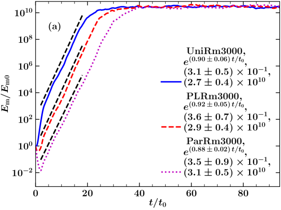
We show the results for varying the seed magnetic field strength or seed Alfvén Mach number in Fig. 6 (models UniMA35000, PLMA35000, and ParMA35000), varying the magnetic Reynolds number in Fig. 7 (models UniRm3000, PLRm3000, and ParRm3000), and varying the sonic Mach number in Fig. 8 (models UniMS10, PLMS10, and ParMS10). For the change in the seed Alfvén Mach number and magnetic Reynolds number, the results (time evolution of magnetic energy, spectra, and PDFs of the component of the magnetic field) follow similar trends as before.
The trends change slightly for . Fig. 8(a) shows a very quick initial amplification of the magnetic field for all three seed-field cases, due to the compression of the magnetic field lines (not seen before for any runs). This is also reflected in the spectra (Fig. 8(b) for ), where the fields on smaller scales are amplified more than on the larger scales (the power is non-zero on all scales for all three seed-field cases). Once the magnetic field reaches the kinematic stage, the spectra for all three seed fields are equal and remain the same also in the saturated stage. The PDFs in the saturated stage are more intermittent than in the kinematic stage, but the PDFs both in the kinematic and saturated stages are more intermittent for the case than for any of the cases (compare the -axis values and the heavy tails at higher values in Fig. 5a and Fig. 8c). However, the growth rate and the structure of the magnetic fields in the kinematic and saturated stages, even for the case, are unaffected by the configuration of the seed field.
The overall conclusions, even with changes in the plasma parameters, remain the same as before: the structure and strength of the seed magnetic fields do not affect the growth rate, final saturation level, shape of the magnetic power spectrum, and the statistical structure of the small-scale dynamo generated magnetic fields. Thus, the detailed properties of the seed field or even their various generation mechanisms are relatively unimportant when studying evolved magnetic fields that were amplified by the turbulent small-scale dynamo.
4 Discussion

From our results, we show that the seed magnetic field information is lost (within a few eddy turnover times, as seen in Fig. 2(a), Fig. 6(a), Fig. 7(a), and Fig. 8(a)). Then the dynamo-generated magnetic field reaches a statistically similar state for all three seed fields, which is determined by the properties of the turbulence (such as Re and ) and magnetic resistivity (or equivalently Rm). This also shows that the small-scale dynamo is very efficient in amplifying (given that Rm is greater than its critical value, ) any non-zero seed field.
4.1 Small-scale magnetic fields generated by the tangling of the large-scale field
If , the small-scale dynamo is inactive. However, for the case with non-zero mean seed field (UniRm100), small-scale magnetic fields can still be generated by the tangling of the large-scale (or mean) uniform seed field (see Appendix A in Seta et al., 2018, for discussion on various mechanisms by which small-scale magnetic fields can be generated). Such a mechanism is only applicable in systems, such as spiral galaxies, where the large-scale field is maintained by other processes, i.e., large-scale dynamo (Krause & Rädler, 1980; Shukurov & Sokoloff, 2008; Chamandy et al., 2014) or cosmic-ray driven dynamo (Parker, 1992; Hanasz et al., 2004). In our simulations, the large-scale uniform field is maintained at all times because the MHD equations (Eq. 1–Eq. 4) preserve the net seed magnetic flux in a triply periodic numerical domain.
We demonstrate the growth of small-scale magnetic fields by the tangling of the uniform seed field in Fig. 9 by choosing . In Fig. 9(a), we show the evolution of magnetic and turbulent kinetic energies for models with all three seed field cases (UniRm100, PLRm100, and ParRm100). The magnetic energy only grows (linearly) for the case UniRm100 and decays for the other two cases (PLRm100 and ParRm100).
Analytically the total magnetic field () in the induction equation can be divided into the small-scale, random () and large-scale, mean () field. Substituting in Eq. 3, we get
| (7) |
Since , in comparison to , varies over a much larger spatial and temporal scales (here, is constant in space and time), we can simplify Eq. 7 further as,
| (8) |
The first term on the right-hand side of the Eq. 8 represents the amplification of the small-scale magnetic field due to the stretching and compression of magnetic field lines by the turbulent velocity. The second term on the right-hand side of the Eq. 8 represents amplification of the magnetic field due to the tangling of the large-scale field by the turbulent velocity. The last term in Eq. 8 represents magnetic diffusion. Initially, for a uniform seed field (UniRm100), the first and third terms in Eq. 8 are negligible since the small-scale field is very small (zero to start with) and the magnetic power is negligible on smaller scales where the diffusion is primarily active. Once the small-scale magnetic field grows, the other two terms in Eq. 8 can no longer be ignored, especially the diffusion term which becomes quite significant because the magnetic power is non-zero on smaller scales. The field eventually reaches a statistically steady-state caused by the competition between tangling and diffusion.
4.2 In the absence of active turbulence
Our main conclusion from this study, namely that the strength and structure of the seed magnetic field do not affect dynamo amplification holds true only for regions with a significant level of turbulence. In contrast, for low-density regions with negligible turbulence, (e.g., voids of the large-scale cosmic structure), the evolved magnetic fields still have imprints of the seed field (can be seen in the results from the IllustrisTNG cosmological simulations; see e.g., figures 14 and 19 in Marinacci et al., 2015). From the observed limits of the magnetic field strengths in voids (Neronov & Vovk, 2010; Tavecchio et al., 2011; Tiede et al., 2020), it is unclear whether they are primordial (early Universe) or developed later in the history of the Universe due to galactic winds (Bertone et al., 2006; Samui et al., 2018) or outflows from AGNs (Furlanetto & Loeb, 2001).
Observations of magnetic fields in young galaxies (Bernet et al., 2008; Mao et al., 2017; Malik et al., 2020) confirm the presence of strong fields, comparable to the magnetic field strengths observed in the Milky Way (Haverkorn, 2015), and in nearby spiral galaxies (Fletcher et al., 2004, 2011; Beck, 2015, 2016). The present observations of magnetic fields, even in young galaxies, cannot help us distinguish between various seed-field generation scenarios (especially astrophysical vs. primordial) because any seed-field information is lost very early on in the evolution. However, primordial magnetic fields can still be studied via other observational probes (see, e.g., table 1 in Subramanian, 2016).
5 Conclusions
We studied the effect of the strength and structure of seed magnetic fields on the small-scale turbulent dynamo action via numerical simulations. Motivated by various seed-field generation mechanisms, we select three possible seed-field configurations: uniform field (, Uni), random field with a power-law spectrum (, PL), and random field with a parabolic spectrum (, Par). Based on our results, we arrive at the following conclusions:
-
•
The magnetic field growth rate in the kinematic stage, and the final saturated amplification level are not affected by the strength and structure of the seed field (Fig. 2(a)).
-
•
The spectrum, though very different for all three seed-field cases, quickly spreads over a range of wave numbers, and is statistically similar in both the kinematic and saturated stages for all three cases (Fig. 3(a)). The computed coherence length of the magnetic field is lower in the kinematic stage as compared to the saturated stage, but is very similar for all three seed-field cases (Fig. 3(b)).
- •
- •
-
•
The seed-field information is lost, since the small-scale turbulent dynamo is very efficient in amplifying seed fields of any form, as long as it is non-zero and the magnetic Reynolds number is greater than its critical value. The details of the seed field or their various generation mechanisms are not important when studying the magnetic field amplified by the small-scale turbulent dynamo.
-
•
Even when the small-scale dynamo action is not active, a weak small-scale magnetic field can be generated and maintained by the tangling of the large-scale magnetic field (if present) (Fig. 9). The tangled small-scale magnetic field in such a case only grows linearly and then saturates once the diffusion term balances the tangling term (Eq. 8).
Acknowledgements
We thank the anonymous referee for a thorough review of this work. A. S. thanks Ramkishor Sharma for interesting discussions on primordial magnetic fields. C. F. acknowledges funding provided by the Australian Research Council (Discovery Project DP170100603 and Future Fellowship FT180100495), and the Australia-Germany Joint Research Cooperation Scheme (UA-DAAD). We further acknowledge high-performance computing resources provided by the Leibniz Rechenzentrum and the Gauss Centre for Supercomputing (grants pr32lo, pr48pi and GCS Large-scale project 10391), the Australian National Computational Infrastructure (grant ek9) in the framework of the National Computational Merit Allocation Scheme and the ANU Merit Allocation Scheme. The simulation software FLASH was in part developed by the DOE-supported Flash Center for Computational Science at the University of Chicago.
Data availability
The data used in this article is available upon request to the corresponding author, Amit Seta ([email protected]).
References
- Batchelor (1950) Batchelor G. K., 1950, Proceedings of the Royal Society of London Series A, 201, 405
- Beck (2015) Beck R., 2015, Astron. Astrophys., 578, A93
- Beck (2016) Beck R., 2016, Ann. Rev. Astron. Astrophys., 24, 4
- Beck et al. (1996) Beck R., Brandenburg A., Moss D., Shukurov A., Sokoloff D., 1996, Ann. Rev. Astron. Astrophys., 34, 155
- Beresnyak (2012) Beresnyak A., 2012, Phys. Rev. Lett., 108, 035002
- Bernet et al. (2008) Bernet M. L., Miniati F., Lilly S. J., Kronberg P. P., Dessauges-Zavadsky M., 2008, Nature, 454, 302
- Bertone et al. (2006) Bertone S., Vogt C., Enßlin T., 2006, Mon. Not. R. Astron. Soc., 370, 319
- Bhat & Subramanian (2013) Bhat P., Subramanian K., 2013, Mon. Not. R. Astron. Soc., 429, 2469
- Bhat & Subramanian (2014) Bhat P., Subramanian K., 2014, Astrophys. J., 791, L34
- Biermann (1950) Biermann L., 1950, Zeitschrift Naturforschung Teil A, 5, 65
- Boldyrev & Cattaneo (2004) Boldyrev S., Cattaneo F., 2004, Phys. Rev. Lett., 92, 144501
- Bouchut et al. (2007) Bouchut F., Klingenberg C., Waagan K., 2007, Numerische Mathematik, 108, 7
- Bouchut et al. (2010) Bouchut F., Klingenberg C., Waagan K., 2010, Numerische Mathematik, 115, 647
- Brandenburg & Subramanian (2005) Brandenburg A., Subramanian K., 2005, Phys. Rep., 417, 1
- Brandenburg et al. (2015) Brandenburg A., Kahniashvili T., Tevzadze A. e. G., 2015, Phys. Rev. Lett., 114, 075001
- Brandenburg et al. (2018) Brandenburg A., Haugen N. E. L., Li X.-Y., Subramanian K., 2018, Mon. Not. R. Astron. Soc., 479, 2827
- Bushby & Favier (2014) Bushby P. J., Favier B., 2014, Astron. Astrophys., 562, A72
- Bushby et al. (2010) Bushby P. J., Proctor M. R. E., Weiss N. O., 2010, in Numerical Modeling of Space Plasma Flows, Astronum-2009. p. 181
- Carilli & Taylor (2002) Carilli C. L., Taylor G. B., 2002, Ann. Rev. Astron. Astrophys., 40, 319
- Cattaneo (1999) Cattaneo F., 1999, Astrophys. J., 515, L39
- Cattaneo & Tobias (2009) Cattaneo F., Tobias S. M., 2009, Journal of Fluid Mechanics, 621, 205
- Chamandy et al. (2014) Chamandy L., Shukurov A., Subramanian K., Stoker K., 2014, Mon. Not. R. Astron. Soc., 443, 1867
- Cho (2014) Cho J., 2014, Astrophys. J., 797, 133
- Cho & Ryu (2009) Cho J., Ryu D., 2009, Astrophys. J., 705, L90
- Cho et al. (2009) Cho J., Vishniac E. T., Beresnyak A., Lazarian A., Ryu D., 2009, Astrophys. J., 693, 1449
- Davies & Widrow (2000) Davies G., Widrow L. M., 2000, Astrophys. J., 540, 755
- Domínguez-Fernández et al. (2019) Domínguez-Fernández P., Vazza F., Brüggen M., Brunetti G., 2019, Mon. Not. R. Astron. Soc., 486, 623
- Dubey et al. (2008) Dubey A., et al., 2008, Challenges of Extreme Computing using the FLASH code. p. 145
- Durrer & Neronov (2013) Durrer R., Neronov A., 2013, A&ARv, 21, 62
- Elmegreen (2009) Elmegreen B. G., 2009, in Andersen J., Nordströara m B., Bland -Hawthorn J., eds, IAU Symposium Vol. 254, The Galaxy Disk in Cosmological Context. pp 289–300 (arXiv:0810.5406), doi:10.1017/S1743921308027713
- Eswaran & Pope (1988) Eswaran V., Pope S. B., 1988, Computers and Fluids, 16, 257
- Favier & Bushby (2012) Favier B., Bushby P. J., 2012, Journal of Fluid Mechanics, 690, 262
- Federrath (2013) Federrath C., 2013, Mon. Not. R. Astron. Soc., 436, 1245
- Federrath (2016) Federrath C., 2016, Journal of Plasma Physics, 82, 535820601
- Federrath et al. (2010) Federrath C., Roman-Duval J., Klessen R. S., Schmidt W., Mac Low M.-M., 2010, Astron. Astrophys., 512, A81
- Federrath et al. (2011) Federrath C., Chabrier G., Schober J., Banerjee R., Klessen R. S., Schleicher D. R. G., 2011, Phys. Rev. Lett., 107, 114504
- Federrath et al. (2014) Federrath C., Schober J., Bovino S., Schleicher D. R. G., 2014, Astrophys. J., 797, L19
- Federrath et al. (2017) Federrath C., et al., 2017, in Crocker R. M., Longmore S. N., Bicknell G. V., eds, IAU Symposium Vol. 322, The Multi-Messenger Astrophysics of the Galactic Centre. pp 123–128 (arXiv:1609.08726), doi:10.1017/S1743921316012357
- Fletcher et al. (2004) Fletcher A., Berkhuijsen E. M., Beck R., Shukurov A., 2004, Astron. Astrophys., 414, 53
- Fletcher et al. (2011) Fletcher A., Beck R., Shukurov A., Berkhuijsen E. M., Horellou C., 2011, Mon. Not. R. Astron. Soc., 412, 2396
- Fryxell et al. (2000) Fryxell B., et al., 2000, ApJS, 131, 273
- Furlanetto & Loeb (2001) Furlanetto S. R., Loeb A., 2001, Astrophys. J., 556, 619
- Gilbert et al. (2016) Gilbert A. D., Mason J., Tobias S. M., 2016, Journal of Fluid Mechanics, 791, 568
- Gnedin et al. (2000) Gnedin N. Y., Ferrara A., Zweibel E. G., 2000, Astrophys. J., 539, 505
- Govoni & Feretti (2004) Govoni F., Feretti L., 2004, International Journal of Modern Physics D, 13, 1549
- Hanasz et al. (2004) Hanasz M., Kowal G., Otmianowska-Mazur K., Lesch H., 2004, Astrophys. J., 605, L33
- Haugen et al. (2004) Haugen N. E., Brandenburg A., Dobler W., 2004, Phys. Rev. E, 70, 016308
- Haverkorn (2015) Haverkorn M., 2015, in Lazarian A., de Gouveia Dal Pino E. M., Melioli C., eds, Astrophysics and Space Science Library Vol. 407, Magnetic Fields in Diffuse Media. p. 483 (arXiv:1406.0283), doi:10.1007/978-3-662-44625-6_17
- Haverkorn et al. (2008) Haverkorn M., Brown J. C., Gaensler B. M., McClure-Griffiths N. M., 2008, Astrophys. J., 680, 362
- Iskakov et al. (2007) Iskakov A. B., Schekochihin A. A., Cowley S. C., McWilliams J. C., Proctor M. R. E., 2007, Phys. Rev. Lett., 98, 208501
- Kazantsev (1968) Kazantsev A. P., 1968, Soviet Journal of Experimental and Theoretical Physics, 26, 1031
- Krause & Rädler (1980) Krause F., Rädler K. H., 1980, Mean-field magnetohydrodynamics and dynamo theory
- Krumholz & Burkhart (2016) Krumholz M. R., Burkhart B., 2016, Mon. Not. R. Astron. Soc., 458, 1671
- Krumholz et al. (2018) Krumholz M. R., Burkhart B., Forbes J. C., Crocker R. M., 2018, Mon. Not. R. Astron. Soc., 477, 2716
- Kulsrud & Anderson (1992) Kulsrud R. M., Anderson S. W., 1992, Astrophys. J., 396, 606
- Kulsrud & Zweibel (2008) Kulsrud R. M., Zweibel E. G., 2008, Reports on Progress in Physics, 71
- Kulsrud et al. (1997a) Kulsrud R., Cowley S. C., Gruzinov A. V., Sudan R. N., 1997a, Phys. Rep., 283, 213
- Kulsrud et al. (1997b) Kulsrud R. M., Cen R., Ostriker J. P., Ryu D., 1997b, Astrophys. J., 480, 481
- Langer & Durrive (2018) Langer M., Durrive J.-B., 2018, Galaxies, 6, 124
- Mac Low & Klessen (2004) Mac Low M.-M., Klessen R. S., 2004, Reviews of Modern Physics, 76, 125
- Malik et al. (2020) Malik S., Chand H., Seshadri T. R., 2020, Astrophys. J., 890, 132
- Mao et al. (2017) Mao S. A., et al., 2017, Nature Astronomy, 1, 621
- Marinacci et al. (2015) Marinacci F., Vogelsberger M., Mocz P., Pakmor R., 2015, Mon. Not. R. Astron. Soc., 453, 3999
- Marinacci et al. (2018) Marinacci F., et al., 2018, Mon. Not. R. Astron. Soc., 480, 5113
- Martins Afonso et al. (2019) Martins Afonso M., Mitra D., Vincenzi D., 2019, Proceedings of the Royal Society A: Mathematical, Physical and Engineering Sciences, 475, 20180591
- Meneguzzi et al. (1981) Meneguzzi M., Frisch U., Pouquet A., 1981, Physical Review Letters, 47, 1060
- Moffatt (1978) Moffatt H. K., 1978, Magnetic field generation in electrically conducting fluids.. Cambridge University Press, Cambridge
- Neronov & Vovk (2010) Neronov A., Vovk I., 2010, Science, 328, 73
- Pakmor et al. (2017) Pakmor R., et al., 2017, Mon. Not. R. Astron. Soc., 469, 3185
- Parker (1992) Parker E. N., 1992, Astrophys. J., 401, 137
- Rees (2005) Rees M. J., 2005, Magnetic Fields in the Early Universe. p. 1, doi:10.1007/11369875_1
- Rieder & Teyssier (2016) Rieder M., Teyssier R., 2016, Mon. Not. R. Astron. Soc., 457, 1722
- Rieder & Teyssier (2017a) Rieder M., Teyssier R., 2017a, Mon. Not. R. Astron. Soc., 471, 2674
- Rieder & Teyssier (2017b) Rieder M., Teyssier R., 2017b, Mon. Not. R. Astron. Soc., 472, 4368
- Rincon (2019) Rincon F., 2019, Journal of Plasma Physics, 85, 205850401
- Ruzmaikin et al. (1988) Ruzmaikin A. A., Sokoloff D. D., Shukurov A. M., eds, 1988, Magnetic fields of galaxies Astrophysics and Space Science Library Vol. 133, doi:10.1007/978-94-009-2835-0.
- Ruzmaikin et al. (1989) Ruzmaikin A., Sokoloff D., Shukurov A., 1989, Mon. Not. R. Astron. Soc., 241, 1
- Samui et al. (2018) Samui S., Subramanian K., Srianand R., 2018, Mon. Not. R. Astron. Soc., 476, 1680
- Schekochihin & Cowley (2006) Schekochihin A. A., Cowley S. C., 2006, Physics of Plasmas, 13, 056501
- Schekochihin & Kulsrud (2001) Schekochihin A. A., Kulsrud R. M., 2001, Physics of Plasmas, 8, 4937
- Schekochihin et al. (2004) Schekochihin A. A., Cowley S. C., Taylor S. F., Maron J. L., McWilliams J. C., 2004, Astrophys. J., 612, 276
- Schlickeiser & Shukla (2003) Schlickeiser R., Shukla P. K., 2003, Astrophys. J. Lett., 599, L57
- Schober et al. (2012a) Schober J., Schleicher D., Federrath C., Klessen R., Banerjee R., 2012a, Phys. Rev. E, 85, 026303
- Schober et al. (2012b) Schober J., Schleicher D., Bovino S., Klessen R. S., 2012b, Phys. Rev. E, 86, 066412
- Schober et al. (2015) Schober J., Schleicher D. R. G., Federrath C., Bovino S., Klessen R. S., 2015, Phys. Rev. E, 92, 023010
- Seta (2019) Seta A., 2019, PhD thesis, Newcastle University, Newcastle Upon Tyne, UK, http://theses.ncl.ac.uk/jspui/handle/10443/4685
- Seta et al. (2015) Seta A., Bhat P., Subramanian K., 2015, Journal of Plasma Physics, 81, 395810503
- Seta et al. (2018) Seta A., Shukurov A., Wood T. S., Bushby P. J., Snodin A. P., 2018, Mon. Not. R. Astron. Soc., 473, 4544
- Seta et al. (2020) Seta A., Bushby P. J., Shukurov A., Wood T. S., 2020, Phys. Rev. Fluids, 5, 043702
- Sharma et al. (2017) Sharma R., Jagannathan S., Seshadri T. R., Subramanian K., 2017, Phys. Rev. D, 96, 083511
- Sharma et al. (2018) Sharma R., Subramanian K., Seshadri T. R., 2018, Phys. Rev. D, 97, 083503
- Shukurov (2004) Shukurov A., 2004, ArXiv Astrophysics e-prints,
- Shukurov & Sokoloff (2008) Shukurov A., Sokoloff D., 2008, in Cardin P., Cugliandolo L., eds, Les Houches, Vol. 88, Dynamos. Elsevier, pp 251 – 299
- Subramanian (1999) Subramanian K., 1999, Phys. Rev. Lett., 83, 2957
- Subramanian (2003) Subramanian K., 2003, Phys. Rev. Lett., 90, 245003
- Subramanian (2016) Subramanian K., 2016, Reports on Progress in Physics, 79, 076901
- Subramanian (2019) Subramanian K., 2019, Galaxies, 7, 47
- Subramanian et al. (1994) Subramanian K., Narasimha D., Chitre S. M., 1994, Mon. Not. R. Astron. Soc., 271, L15
- Sur et al. (2012) Sur S., Federrath C., Schleicher D. R. G., Banerjee R., Klessen R. S., 2012, Mon. Not. R. Astron. Soc., 423, 3148
- Sur et al. (2018) Sur S., Bhat P., Subramanian K., 2018, Mon. Not. R. Astron. Soc., 475, L72
- Tavecchio et al. (2011) Tavecchio F., Ghisellini G., Bonnoli G., Foschini L., 2011, Mon. Not. R. Astron. Soc., 414, 3566
- Tiede et al. (2020) Tiede P., Broderick A. E., Shalaby M., Pfrommer C., Puchwein E., Chang P., Lamberts A., 2020, Astrophys. J., 892, 123
- Tzeferacos et al. (2018) Tzeferacos P., et al., 2018, Nature Communications, 9, 591
- Vaĭnshteĭn & Zel’dovich (1972) Vaĭnshteĭn S. I., Zel’dovich Y. B., 1972, Soviet Physics Uspekhi, 15, 159
- Vazza et al. (2018) Vazza F., Brunetti G., Brüggen M., Bonafede A., 2018, Mon. Not. R. Astron. Soc., 474, 1672
- Waagan et al. (2011) Waagan K., Federrath C., Klingenberg C., 2011, J. Comput. Phys., 230, 3331
- Weiss (1966) Weiss N. O., 1966, Proceedings of the Royal Society of London Series A, 293, 310
- Widrow (2002) Widrow L. M., 2002, Reviews of Modern Physics, 74, 775
- Widrow et al. (2012) Widrow L. M., Ryu D., Schleicher D. R. G., Subramanian K., Tsagas C. G., Treumann R. A., 2012, SSRv, 166, 37
- Zeldovich et al. (1990) Zeldovich Ya. B., Ruzmaikin A. A., Sokoloff D. D., 1990, The Almighty Chance. World Scientific, Singapore