Sedimenting Elastic Filaments in Turbulent Flows
Abstract
We investigate the gravitational settling of a long, model elastic filament in homogeneous isotropic turbulence. We show that the flow produces a strongly fluctuating settling velocity, whose mean is moderately enhanced over the still-fluid terminal velocity, and whose variance has a power-law dependence on the filament’s weight but is surprisingly unaffected by its elasticity. In contrast, the tumbling of the filament is shown to be closely coupled to its stretching, and manifests as a Poisson process with a tumbling time that increases with the elastic relaxation time of the filament.
Sediments in turbulent flows are commonplace in nature and industry. Even so, theoretical progress in understanding how objects settle under gravity while being buffeted by a turbulent carrier flow is recent. Even in the simplest case of tiny rigid spherical particles, the interaction of these forces is rather intricate and leads to an enhancement of the settling velocity over its value in a still fluid—a fact that has been theoretically understood and quantified over just the past decade or so Maxey (1987); Wang and Maxey (1993); Aliseda et al. (2002); Ghosh et al. (2005); Ayala et al. (2008); Davila and Hunt (2001); Bec et al. (2014). More recent work has addressed the issue of how spheroidal particles, with additional rotational degrees of freedom, orient themselves while settling Gustavsson et al. (2017); Anand et al. (2020). A common feature of these prior studies is that they are limited to rigid particles whose sizes, regardless of their anisotropy, are much smaller than the dissipative Kolmogorov scale of the flow. These constraints are certainly meaningful for a wide variety of applications, such as understanding the initiation of rain in warm clouds Vaillancourt and Yau (2000); Falkovich et al. (2002); Shaw (2003); Bodenschatz et al. (2010); Monchaux et al. (2012) and the radiative properties of cold clouds Baran and Francis (2004); Gallagher et al. (2005); Pandit et al. (2015); Voth and Soldati (2017), which involve, respectively, turbulent suspensions of spherical water droplets and non-spherical ice crystals.
However, sediments that are both deformable and larger than the Kolmogorov scale are just as ubiquitous. One important example is the sedimentation of long deformable filaments, wherein flow-induced deformation modifies the net drag force experienced by the filament Alben et al. (2002), thus coupling the dynamics of conformation to settling. This problem has been recently addressed for low Reynolds number, non-turbulent flows Marchetti et al. (2018). However, understanding the gravitational settling of filaments when the carrier flow is turbulent (as encountered in papermaking (Lundell et al., 2011) and the fields of marine ecology and pollution Barnes et al. (2009); Lusher (2015); Stelfox et al. (2016); Lebreton et al. (2018)) remains an important open problem.
In this paper, we address this issue through a combination of scaling analysis and detailed numerical simulations on a model elastic filament in a homogeneous and isotropic turbulent flow. In particular, we show that the turbulent flow produces strong fluctuations in the settling velocity, while moderately enhancing its mean value over the terminal value in a still-fluid. We theoretically derive how the normalised variance of the settling velocity scales with the elasticity and inertia (mass) of the filament, as well as with the relative strengths of the accelerations due to gravity and turbulence. Our estimates are then verified through detailed numerical simulations. Furthermore, borrowing ideas from the persistence problem of non-equilibrium statistical physics, we uncover a close connection between the two internal motions of tumbling and stretching, which accompany the unsteady yet inevitable descent of the filament.
A simple model of a long filament, which retains enough internal structure to exhibit both elasticity and inertia, is a chain of heavy inertial particles connected through elastic springs Bird et al. (1977). Such chains are a useful framework to understand the intricate interplay between elasticity and turbulent mixing Picardo et al. (2018); Singh et al. (2020); Picardo et al. (2020) and provide insights which complement those obtained from other models of fibres Brouzet et al. (2014); Verhille and Bartoli (2016); Rosti et al. (2018); Allende et al. (2018). In this context, the most striking feature of filaments such as those we study is the manner in which they preferentially sample the geometry of a turbulent flow: in the inertia-less (neutrally buoyant) limit, such chains preferentially sample the vortical regions of the flow, in both two and three dimensions (3D) though for different reasons Picardo et al. (2018, 2020). This prediction, for the case of rigid chains in 3D, was recently confirmed experimentally (Oehmke et al., 2020). The introduction of inertia (without gravity), counter-acts this tendency due to centrifugal expulsion from vortices and decorrelation from the flow, resulting in rather distinct dynamics Singh et al. (2020). Here, we account for gravitational acceleration and investigate the settling dynamics of these elasto-inertial chains.
We model a filament of mass as a chain of spherical beads. Considering to be the mass density of the filament, we distribute the mass uniformly over the beads, each of radius , so that . The beads are then characterised by a Stokesian relaxation time , where and are the density and kinematic viscosity of the carrier fluid. Each bead, positioned instantaneously at , is connected to its nearest neighbours through (phantom) elastic links with which we associate a relaxation time scale (yielding an effective elastic time scale for the filament Jin and Collins (2007); Picardo et al. (2018)), thus rendering our elasto-inertial chains extensible (and fully flexible). The dynamics of these model filaments are then completely determined by the coupled equations of motion for the inter-bead separation vectors and the center-of-mass :
| (1) | ||||
| (2) | ||||
Here, we use the FENE (finitely extensible nonlinear elastic) interaction , with a prescribed maximum inter-bead length , to model the springs. Independent white noises , with a coefficient , are imposed on the beads to set the equilibrium length for each segment of our filament (in the absence of flow). We choose a coordinate system such that the acceleration due to gravity acts along the negative -axis; the resulting gravitational forces acting on the beads cancel out from Eq. (1) but still have an implicit effect on the dynamics of segments, via their action on the motion of the center-of-mass (which in turn determines the velocities sampled by the beads). Finally, the time-scales and , as well as the acceleration due to gravity , allow us to define non-dimensional numbers in terms of analogous (small-scale) quantities of the carrier turbulent flow, namely the Kolomogorov time and acceleration , where is the mean energy dissipation rate of the flow. The dynamics of our filaments are thus completely determined by the Stokes number (a measure of the inertia), the Froude number (a measure of the force of gravity), and the Weissenberg number (a measure of elasticity).
Note that this simple model disregards inter-bead, hydrodynamic and excluded volume interactions, as well as bending stiffness (Picardo et al., 2020), in an effort to more clearly reveal the fundamental interplay between elasticity, inertia, and gravitational and turbulent acceleration. It is important to point out that other models of filament dynamics, particularly in the context of turbulent transport, are available Brouzet et al. (2014); Verhille and Bartoli (2016); Rosti et al. (2018); Allende et al. (2018). However, studies for low Reynolds number flow show Marchetti et al. (2018) that the bead-spring approach to filaments still remains an important framework Cosentino Lagomarsino et al. (2005); Schlagberger and Netz (2005); Llopis et al. (2007); Delmotte et al. (2015) because of the limitations of models based on slender-body theory Cox (1970); Xu and Nadim (1994).
In our direct numerical simulations, we solve Eqs (1)-(2), using a second-order Runge-Kutta scheme, together and simultaneously with the three-dimensional, incompressible Navier-Stokes equations, driven to a statistically stationary state by using a constant energy injection scheme. To simulate the carrier flow, we use a de-aliased pseudo-spectral algorithm, spatially discretize the Navier-Stokes equations on a 2 periodic cubic box with collocation points, and use a second-order slaved Adams-Bashforth scheme for time integration James and Ray (2017). The fluid velocity obtained on the regular periodic grid is interpolated, using trilinear interpolation, to obtain the velocity at the bead positions. We choose the coefficient of viscosity to obtain a Taylor-scale Reynolds number . We evolve an ensemble of filaments, each with an equilibrium length and beads (we have checked that our results remain qualitatively unchanged if we use a fewer number of beads, ), and consider various values of , and .
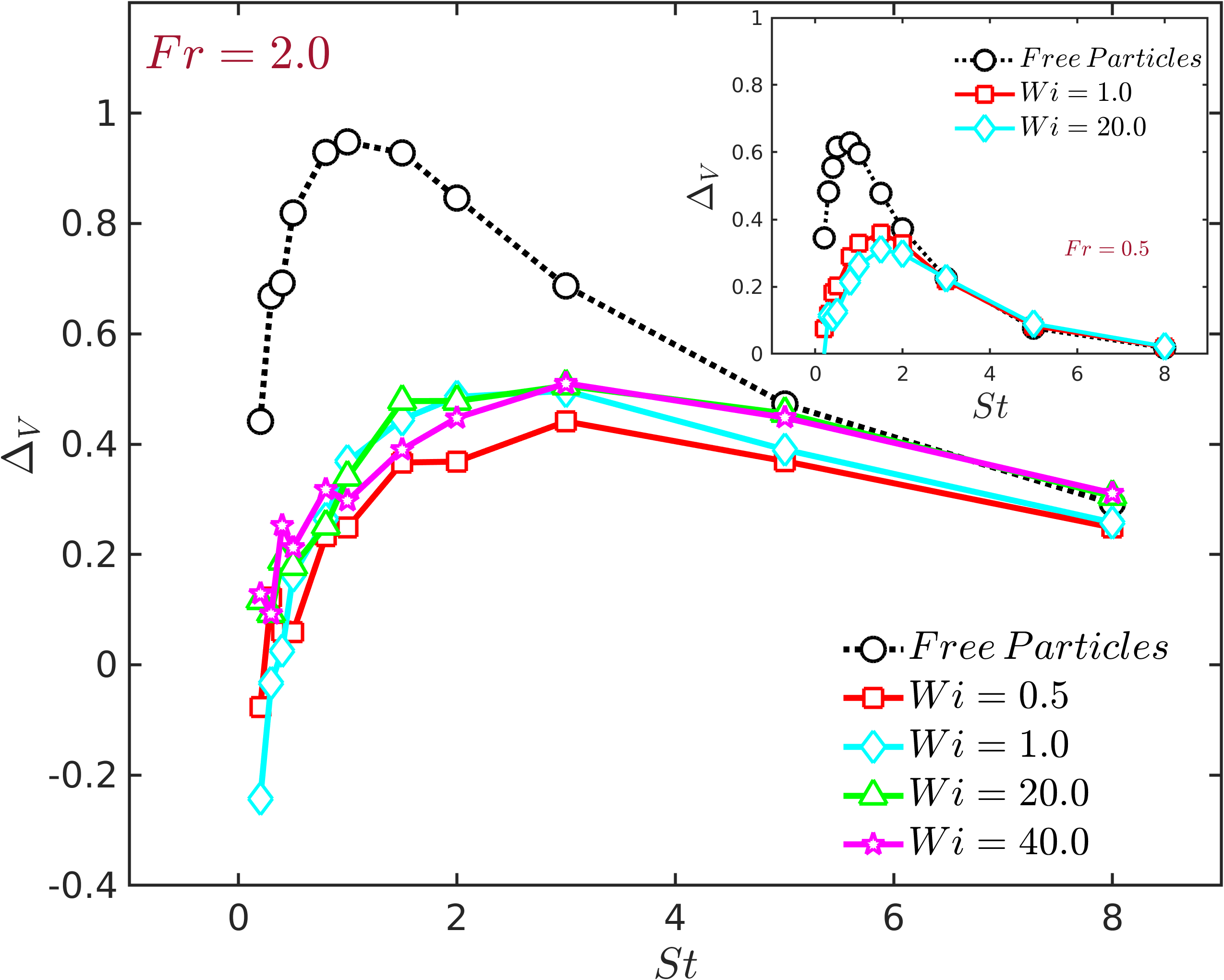
We begin our study by examining the fluctuating settling velocities of the filaments. Let us first consider the mean value , where the angular brackets denote an average over the ensemble of chains and over time in the statistically stationary state. From Eq. (2), denoting as the vertical acceleration in the direction, the assumption of a mean settling velocity implies, by definition, that . Furthermore, since the noises are independent and of zero-mean, we obtain , where is the terminal settling velocity in a still-fluid, and is the average -component of the fluid velocity field sampled by the filament. If an object uniformly samples the flow, as tracer particles do, then . However, this is typically not the case for non-tracers: Heavy inertial particles (with ) are known to preferentially sample descending regions of the flow, leading to and thus an enhanced mean settling velocity. The magnitude of this effect, which may be quantified through , varies non-monotonically with as explained in (Bec et al., 2014).
Now, as instantiated by our model, a filament can be thought of as a string of elastically-linked, inertial particles. So, how does this internal linking impact the mean settling velocity of filaments? Figure 1 answers this question by presenting simulation results of as a function of , for filaments with (see the inset for ) and various values of , as well as for free inertial particles (whose dynamics are given by Eq. (2) with and ). Clearly, the links counter-act the preferential sampling behaviour of inertial particles, resulting in a weaker enhancement of for filaments. Indeed, at very small and for small to moderate , becomes negative and these filaments settle slightly slower than they would in a still fluid. Figure 1 also suggests that the settling velocity is relatively insensitive to the elasticity of the filaments, a rather surprising observation which is reinforced below by considering the fluctuations about the mean value.
The probability distribution function (pdf) of , illustrated in the inset of Fig. 2, shows that the turbulent flow can produce strong temporal fluctuations—much greater than —which become increasingly large and non-Gaussian (the black lines are Gaussian fits) as increases (the relevance of this ratio becomes clear below). The magnitude of these fluctuations is best quantified through the normalised variance of the distribution. To obtain a theoretical estimate for this variance, we use Eq. (2) to calculate the second moment of the settling velocity . Noting that , where the subscript denotes the -components of the noise and is a constant (which absorbs the factor) with the dimension of inverse time, we obtain , which leads to the non-dimensional, normalised variance
| (3) |
where, to extract the leading order behaviour, we set to zero (the validity of this approximation is addressed later) and use .
This result is further simplified by the observation, from our simulations, that , where is the mean kinetic energy of the flow. Furthermore, the small additive contribution of the noise to the variance, , is not relevant to understanding the effect of the turbulent flow on settling. (Indeed, one could use a non-stochastic, fixed equilibrium length, via a spring force proportional to , without affecting the qualitative dynamics of the chains in flow Picardo et al. (2020).) It follows, therefore, that ; the variance only depends on a single settling factor , which is the ratio of the still-fluid terminal settling velocity to the Kolmogorov-scale velocity of the turbulent flow .
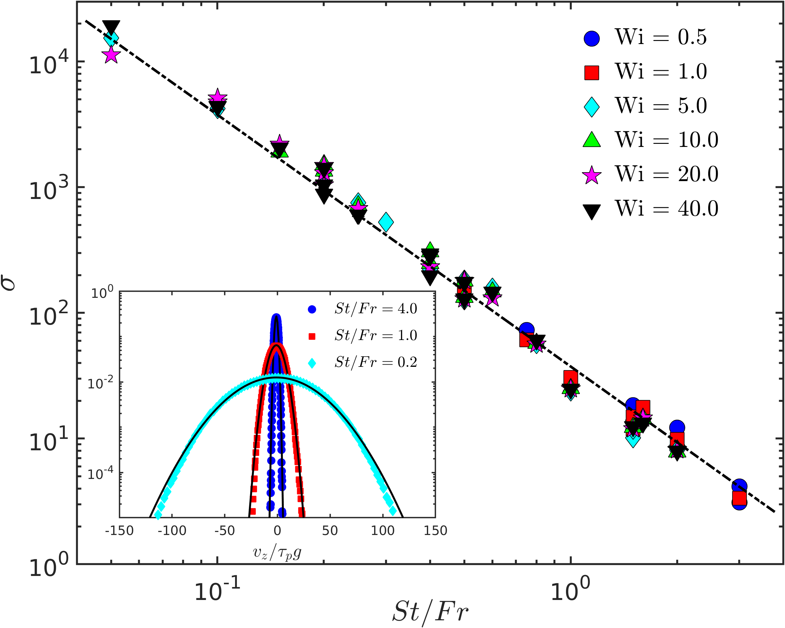
Motivated by this scaling result, we plot the value of obtained from our simulations, carried out by varying , and independently over a range of values, against in Fig. 2. We see that the leading order behaviour of the variance matches the scaling prediction (dotted line) remarkably well, over a wide range of . Clearly, the extent of elasticity and therefore the stretching of the filament does not appreciably impact the settling velocity statistics.
Before proceeding, it is useful to revisit the approximation which lead to Eq. (3). While our simulation data does not allow us direct access to this quantity, we can estimate its value by calculating the residual obtained on substituting our data into Eq. (3). We find (not shown) that is practically independent of , and although it has non-negligible values they are not large enough to disrupt the leading-order scaling with , as is evident in Fig. 2.
So far, we have only considered the settling of the filament as a whole. However, unlike for instance spherical particles, these filaments have additional internal degrees of freedom which raise new questions, of which perhaps the most interesting is to understand how the filaments tumble as they descend through the turbulent flow. It is useful to recall that the tumbling of individual polymers—small elastic chains unaffected by inertia or gravity—has been studied in the context of simple shear flows Gerashchenko and Steinberg (2006); Celani et al. (2005).
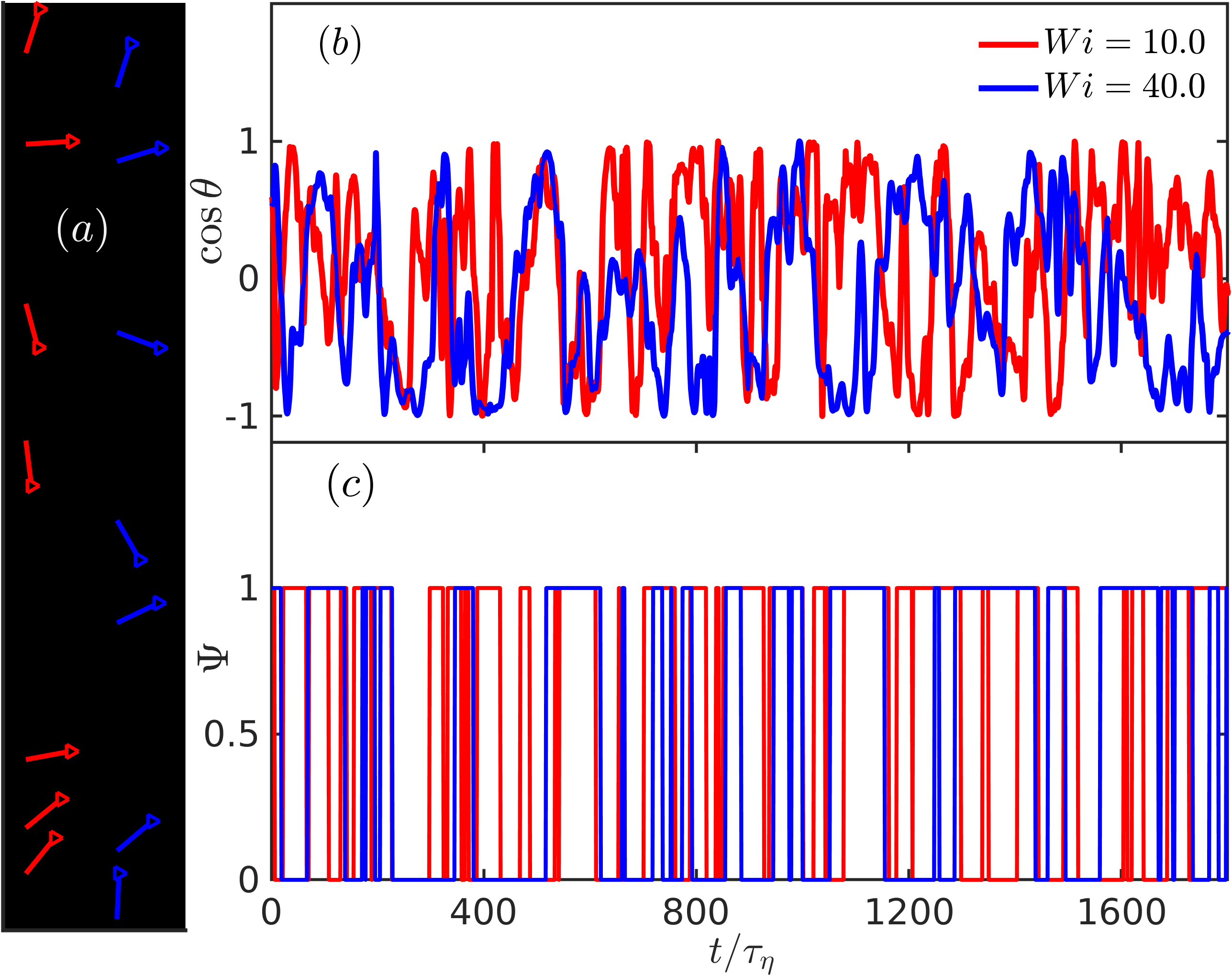
To study tumbling quantitatively, we consider the dynamics of the end-to-end vector . In Fig. 3(a), we show typical time traces of the end-to-end vector projected on a two-dimensional plane, for two sedimenting filaments with different (and , ). Clearly the filaments undergo complicated rotational dynamics accompanied by tumbling events. This behaviour is quantified through the cosine of the angle made by with the -axis, via , where . In Fig. 3(b), we show plots of the time-series of for the two filaments shown in panel (a). This time series illustrates the seemingly continuous changes in the orientation of the settling filaments with a suggestion that less elastic filaments tumble more frequently. Such observations naturally lead us to (a) suitably define the state of the filament as being either “up” or “down” and (b) to characterise the transitions between these two states.
We define the up and down states as for and for , respectively. The apparently random switching between the two states, clearly illustrated in Fig 3(c), is quantified by calculating the pdfs () of the residence time over which the filaments remain up (down). These distributions yield the probability of a filament in an up (or down) state to continue to remain in the same state for a duration of . We recall that questions of this sort—the so-called persistence problems—have a special importance in areas of non-equilibrium statistical physics Majumdar et al. (1996); Derrida et al. (1996); Majumdar (1999); Bray et al. (2013) and have, more recently, been adapted to understand the geometrical aspects of turbulent flows Perlekar et al. (2011); Kadoch et al. (2011); Bhatnagar et al. (2016).
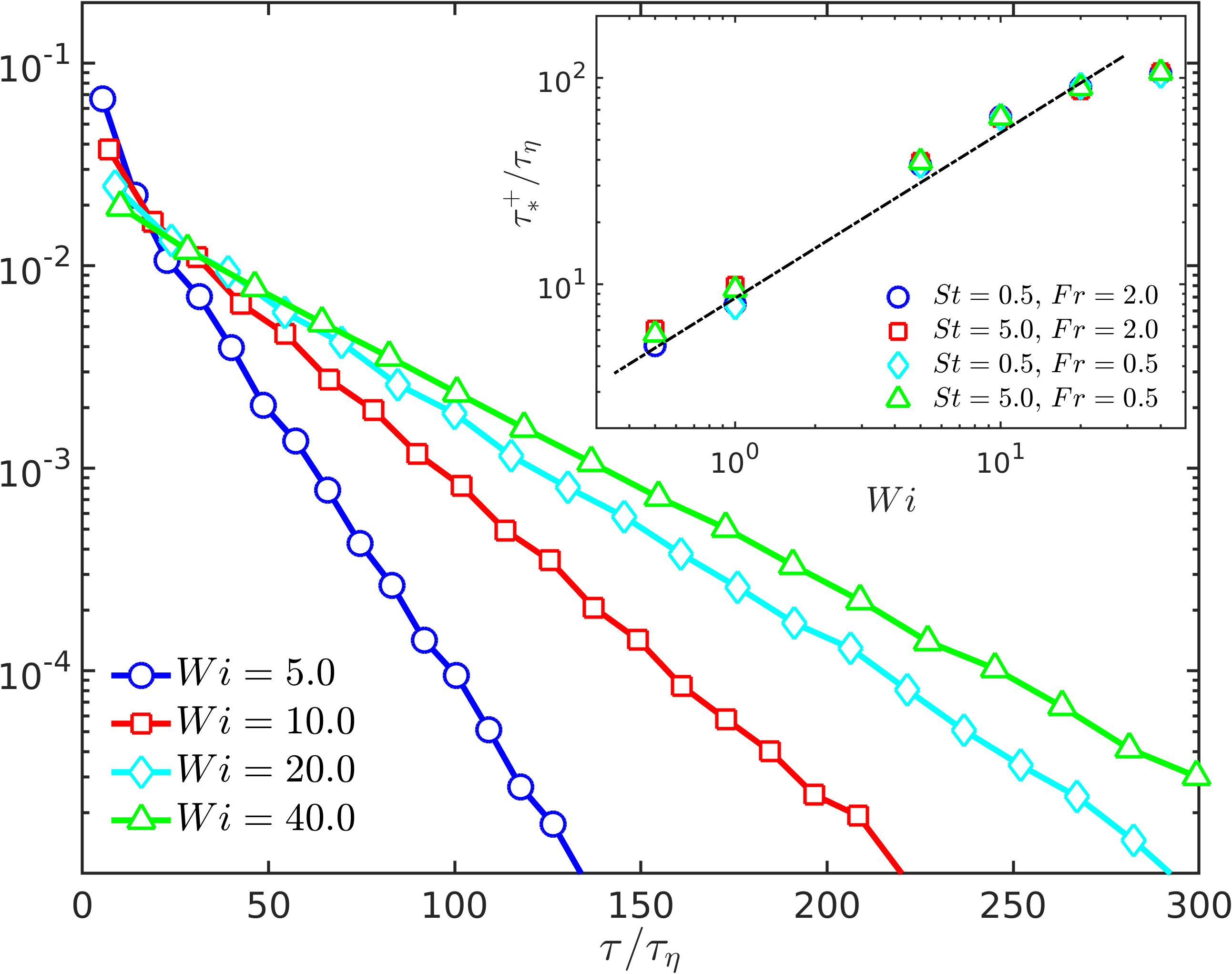
In Fig. 4, we show semi-log plots of for filaments with , but different degrees of elasticity. [We have confirmed, by varying the range of angles which define an up or down state, that the precise definition of these states does not affect the results qualitatively; furthermore, and hence , because the problem is symmetric to the transformation which reverses the end-to-end vector.] These distributions clearly show an exponential fall-off Celani et al. (2005): , which indicates that tumbling manifests as a Poisson process. The characteristic time scale has a weak dependence on and , but increases systematically (see Ref. Celani et al. (2005) for single polymers in a shear flow) with , as seen in the inset of Fig. 4.
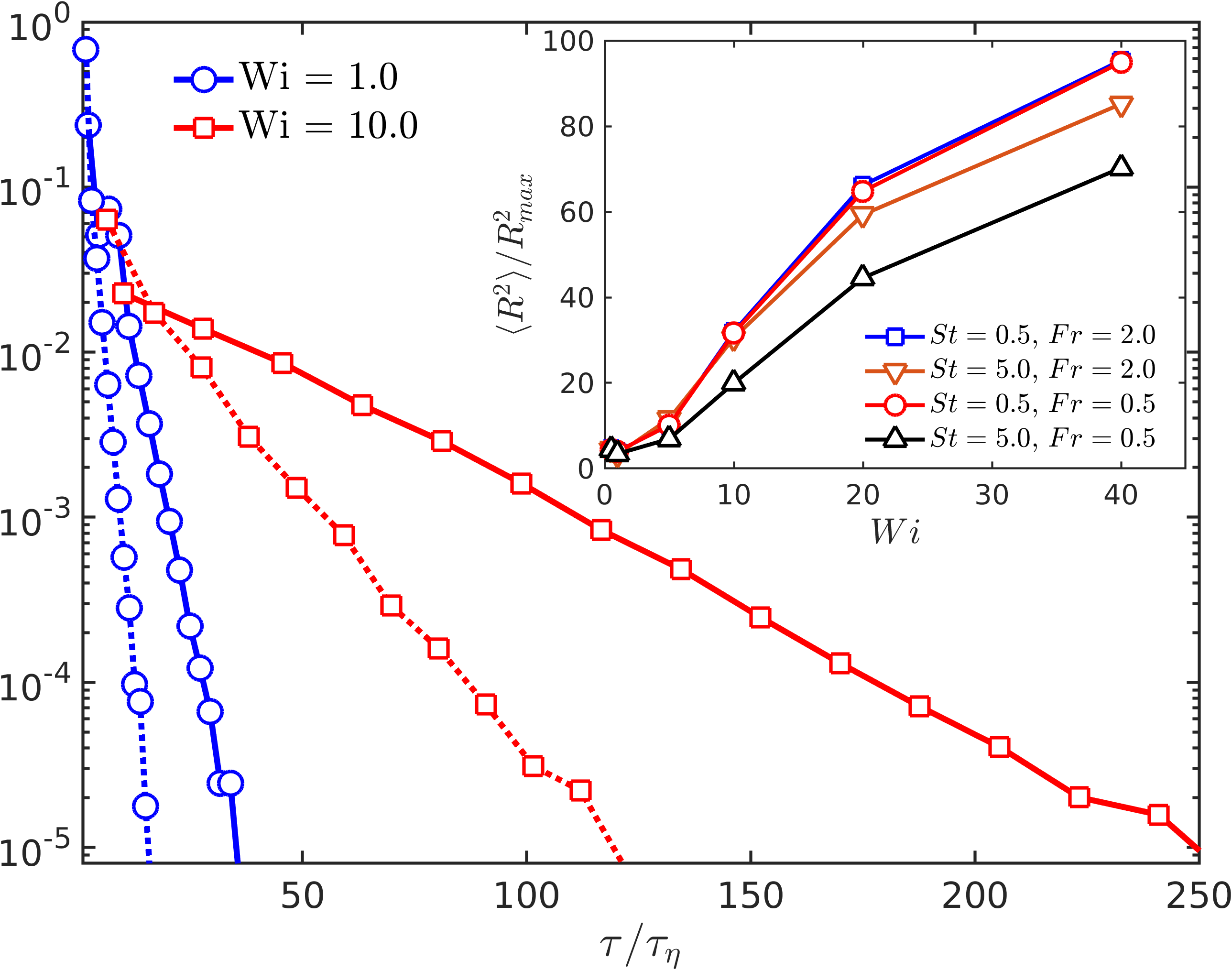
Why do more extensible filaments require longer times to tumble? The answer lies in the connection between the dynamic length of a filament and its tumbling. We expect a highly stretched, long filament that spans multiple flow eddies to have a lower probability of experiencing the sequence of coordinated drag forces required to cause a transition in its orientation. To test this hypothesis, we calculate the average end-to-end length of a filament over each interval of time spent in the up state . When a transition occurs, we record along with the persistence time , which then allows us to obtain the pdf of conditioned on the time-averaged length of the filament. Fig 5 shows these conditioned pdfs for relatively short (dashed line) and long (solid line) filaments, defined as those with and (), where the values of the thresholds depend on and are given in the figure caption (small variations in these values do not affect our conclusions). Two values of are considered, and in both cases we see that when filaments are more stretched they do indeed take a longer time to tumble. (Note that a similar inverse relationship between length and tumbling rate has been recently observed in experiments on rigid, neutrally buoyant fibres in isotropic turbulence (Oehmke et al., 2020).) Now, as increases, the filaments become more extensible and the distribution of broadens. This is demonstrated by the inset of Fig 5, which presents the variation of with , for all chains in the ensemble over all time. As a result, a larger filament is much more likely to be in a highly stretched state, which explains its tendency to persist in a given orientation for a longer time before tumbling. The consequent increase of with , shown in the inset of Fig. 4, appears to follow a power-law (the fitted dashed-line has an exponent of ) for small to moderate , but then begins to level-off at large , as the filament approaches its maximum length.
To summarise, we have analyzed two complementary aspects of the dynamics of long and heavy, elastic filaments in a turbulent flow: the fluctuating settling velocity, and the transitions in vertical orientation associated with tumbling. For a given turbulent flow, we have found, rather surprisingly, that to leading order the weight of the filament only impacts its settling velocity (via the dependence of and the scaling of ) while the elasticity and consequent stretching of the filament only affects its tumbling.
The Poisson distribution of tumbling times, uncovered by our persistence analysis, brings to mind the Poissonian back-and-forth motion of filamentary, motile microorganisms. This tumbling-like motion is thought to be an efficient strategy for foraging Luchsinger et al. (1999); Stocker (2011), but given that the Reynolds number of oceanic turbulence Jimenez (1997) is similar to that in our study, it is tempting to consider in future works whether the tumbling of marine filamentary microorganisms are a consequence of active strategy or physical inevitability. Admittedly, these microorganisms are motile and much smaller than our filaments; nevertheless, our results should motivate work on longer marine organisms and their journey as they settle in the ocean. Furthermore, this study is relevant to the sedimentation of passive marine pollutants, such as plastic debris from fishing gear (Stelfox et al., 2016; Lebreton et al., 2018), as well as to fibre suspensions in industry (Lundell et al., 2011).
Acknowledgements.
We are grateful to Dario Vincenzi for many insightful discussions and for introducing us to this problem. RKS and SSR also thank A. Kundu for useful discussions. The simulations were performed on the ICTS clusters Contra and Tetris as well as the work stations from the project ECR/2015/000361: Goopy and Bagha. SSR and RKS acknowledge the support of the DAE, Govt. of India, under project no. 12-R&D-TFR-5.10-1100 and SSR is grateful to the DST (India) project MTR/2019/001553 for financial help. JRP is thankful for support from the IIT-Bombay IRCC Seed Grant.References
- Maxey (1987) M. Maxey, J. Fluid Mech. 174, 441 (1987).
- Wang and Maxey (1993) L.-P. Wang and M. Maxey, J. Fluid Mech. 256, 27 (1993).
- Aliseda et al. (2002) A. Aliseda, A. Cartellier, F. Hainaux, and J. C. Lasheras, J. Fluid Mech. 468, 77–105 (2002).
- Ghosh et al. (2005) S. Ghosh, J. Dávila, J. Hunt, A. Srdic, H. Fernando, and P. Jonas, Proceedings of the Royal Society A: Mathematical, Physical and Engineering Sciences 461, 3059 (2005).
- Ayala et al. (2008) O. Ayala, B. Rosa, L.-P. Wang, and W. Grabowski, New J. Phys. 10, 075015 (2008).
- Davila and Hunt (2001) J. Davila and J. Hunt, J. Fluid Mech. 440, 117 (2001).
- Bec et al. (2014) J. Bec, H. Homann, and S. S. Ray, Phys. Rev. Lett. 112, 184501 (2014).
- Gustavsson et al. (2017) K. Gustavsson, J. Jucha, A. Naso, E. Lévêque, A. Pumir, and B. Mehlig, Phys. Rev. Lett. 119, 254501 (2017).
- Anand et al. (2020) P. Anand, S. S. Ray, and G. Subramanian, Phys. Rev. Lett. 125, 034501 (2020).
- Vaillancourt and Yau (2000) P. A. Vaillancourt and M. K. Yau, Bulletin of the American Meteorological Society 81, 285 (2000).
- Falkovich et al. (2002) G. Falkovich, A. Fouxon, and M. G. Stepanov, Nature 419, 151 (2002).
- Shaw (2003) R. A. Shaw, Annual Review of Fluid Mechanics 35, 183 (2003).
- Bodenschatz et al. (2010) E. Bodenschatz, S. P. Malinowski, R. A. Shaw, and F. Stratmann, Science 327, 970 (2010).
- Monchaux et al. (2012) R. Monchaux, M. Bourgoin, and A. Cartellier, Int. J. Multiph. Flow 40, 1 (2012).
- Baran and Francis (2004) A. J. Baran and P. N. Francis, Quarterly Journal of the Royal Meteorological Society 130, 763 (2004).
- Gallagher et al. (2005) M. W. Gallagher, P. J. Connolly, J. Whiteway, D. Figueras-Nieto, M. Flynn, T. W. Choularton, K. N. Bower, C. Cook, R. Busen, and J. Hacker, Quarterly Journal of the Royal Meteorological Society 131, 1143 (2005).
- Pandit et al. (2015) A. K. Pandit, H. S. Gadhavi, M. Venkat Ratnam, K. Raghunath, S. V. B. Rao, and A. Jayaraman, Atmospheric Chemistry and Physics 15, 13833 (2015).
- Voth and Soldati (2017) G. A. Voth and A. Soldati, Annual Review of Fluid Mechanics 49, 249 (2017).
- Alben et al. (2002) S. Alben, M. Shelley, and J. Zhang, Nature 420, 479 (2002).
- Marchetti et al. (2018) B. Marchetti, V. Raspa, A. Lindner, O. du Roure, L. Bergougnoux, E. Guazzelli, and C. Duprat, Phys. Rev. Fluids 3, 104102 (2018).
- Lundell et al. (2011) F. Lundell, L. D. Soderberg, and P. H. Alfredsson, Annu. Rev. Fluid Mech 43, 195 (2011).
- Barnes et al. (2009) D. K. A. Barnes, F. Galgani, R. C. Thompson, and M. Barlaz, Philosophical Transactions of the Royal Society B: Biological Sciences 364, 1985 (2009).
- Lusher (2015) A. Lusher, “Microplastics in the marine environment: Distribution, interactions and effects,” in Marine Anthropogenic Litter, edited by M. Bergmann, L. Gutow, and M. Klages (Springer International Publishing, Cham, 2015) pp. 245–307.
- Stelfox et al. (2016) M. Stelfox, J. Hudgins, and M. Sweet, Marine Pollution Bulletin 111, 6 (2016).
- Lebreton et al. (2018) L. Lebreton, B. Slat, F. Ferrari, B. Sainte-Rose, J. Aitken, R. Marthouse, S. Hajbane, S. Cunsolo, A. Schwarz, A. Levivier, K. Noble, P. Debeljak, H. Maral, R. Schoeneich-Argent, R. Brambini, and J. Reisser, Sci. Rep. 8, 4666 (2018).
- Bird et al. (1977) R. B. Bird, C. F. Curtiss, R. C. Armstrong, and O. Hassager, Dynamics of Polymeric Liquids (John Wiley and Sons, New York, 1977).
- Picardo et al. (2018) J. R. Picardo, D. Vincenzi, N. Pal, and S. S. Ray, Phys. Rev. Lett. 121, 244501 (2018).
- Singh et al. (2020) R. Singh, M. Gupta, J. R. Picardo, D. Vincenzi, and S. S. Ray, Phys. Rev. E 101, 053105 (2020).
- Picardo et al. (2020) J. R. Picardo, R. Singh, S. S. Ray, and D. Vincenzi, Phil. Trans. R. Soc. A. 378, 20190405 (2020).
- Brouzet et al. (2014) C. Brouzet, G. Verhille, and P. Le Gal, Phys. Rev. Lett. 112, 074501 (2014).
- Verhille and Bartoli (2016) G. Verhille and A. Bartoli, Exp. Fluids 57, 117 (2016).
- Rosti et al. (2018) M. E. Rosti, A. A. Banaei, L. Brandt, and A. Mazzino, Phys. Rev. Lett. 121, 044501 (2018).
- Allende et al. (2018) S. Allende, C. Henry, and J. Bec, Phys. Rev. Lett. 121, 154501 (2018).
- Oehmke et al. (2020) T. B. Oehmke, A. D. Bordoloi, E. Variano, and G. Verhille, ArXiv e-prints (2020), arXiv:2011.08546 .
- Jin and Collins (2007) S. Jin and L. R. Collins, New J. Phys. 9, 360 (2007).
- Cosentino Lagomarsino et al. (2005) M. Cosentino Lagomarsino, I. Pagonabarraga, and C. P. Lowe, Phys. Rev. Lett. 94, 148104 (2005).
- Schlagberger and Netz (2005) X. Schlagberger and R. R. Netz, Europhysics Letters (EPL) 70, 129 (2005).
- Llopis et al. (2007) I. Llopis, I. Pagonabarraga, M. Cosentino Lagomarsino, and C. P. Lowe, Phys. Rev. E 76, 061901 (2007).
- Delmotte et al. (2015) B. Delmotte, E. Climent, and F. Plouraboué, Journal of Computational Physics 286, 14 (2015).
- Cox (1970) R. G. Cox, J. Fluid Mech. 44, 791–810 (1970).
- Xu and Nadim (1994) X. Xu and A. Nadim, Physics of Fluids 6, 2889 (1994).
- James and Ray (2017) M. James and S. S. Ray, Sci. Rep. 7, 12231 (2017).
- Gerashchenko and Steinberg (2006) S. Gerashchenko and V. Steinberg, Phys. Rev. Lett. 96, 038304 (2006).
- Celani et al. (2005) A. Celani, A. Puliafito, and K. Turitsyn, Europhysics Letters (EPL) 70, 464 (2005).
- Majumdar et al. (1996) S. N. Majumdar, C. Sire, A. J. Bray, and S. J. Cornell, Phys. Rev. Lett. 77, 2867 (1996).
- Derrida et al. (1996) B. Derrida, V. Hakim, and R. Zeitak, Phys. Rev. Lett. 77, 2871 (1996).
- Majumdar (1999) S. N. Majumdar, Current Science 77, 370 (1999).
- Bray et al. (2013) A. J. Bray, S. N. Majumdar, and G. Schehr, Advances in Physics 62, 225 (2013).
- Perlekar et al. (2011) P. Perlekar, S. S. Ray, D. Mitra, and R. Pandit, Phys. Rev. Lett. 106, 054501 (2011).
- Kadoch et al. (2011) B. Kadoch, D. del Castillo-Negrete, W. J. T. Bos, and K. Schneider, Phys. Rev. E 83, 036314 (2011).
- Bhatnagar et al. (2016) A. Bhatnagar, A. Gupta, D. Mitra, R. Pandit, and P. Perlekar, Phys. Rev. E 94, 053119 (2016).
- Luchsinger et al. (1999) R. H. Luchsinger, B. Bergersen, and J. G. Mitchell, Biophysical Journal 77, 2377 (1999).
- Stocker (2011) R. Stocker, Proceedings of the National Academy of Sciences 108, 2635 (2011).
- Jimenez (1997) J. Jimenez, Scientia Marina 61, 47 (1997).