Secure Outage Analysis of RIS-Assisted Communications with Discrete Phase Control
Abstract
This correspondence investigates a reconfigurable intelligent surface (RIS)-assisted wireless communication system with security threats. The RIS is deployed to enhance the secrecy outage probability (SOP) of the data sent to a legitimate user. By deriving the distributions of the received signal-to-noise-ratios (SNRs) at the legitimate user and the eavesdropper, we formulate, in a closed-form expression, a tight bound for the SOP under the constraint of discrete phase control at the RIS. The SOP is characterized as a function of the number of antenna elements, , and the number of discrete phase choices, . It is revealed that the performance loss in terms of SOP due to the discrete phase control is ignorable for large when . In addition, we explicitly quantify this SOP loss when binary phase shifts with is utilized. It is identified that increasing the RIS antenna elements by times can achieve the same SOP with binary phase shifts as that by the RIS with ideally continuous phase shifts. Numerical simulations are conducted to verify the accuracy of these theoretical observations.
Index Terms:
Reconfigurable intelligent surface (RIS), physical layer security, secrecy outage probability, discrete phase shifts.I Introduction
Reconfigurable intelligent surface (RIS) is a metasurface that consists of a large number of passive reflecting elements with integrated low power electronics [1][2]. A main feature of an RIS is that the amplitude and phase of each reflecting element can be independently controlled through software, thereby realizing passive beamforming (BF) for improving the signal quality at intended receivers. Due to these merits, RISs have been considered for various wireless applications, e.g., in millimeter-wave (mmWave) [3] and Terahertz (THz) [4] communications, to enhance spectral and energy efficiencies [5].
In recent years, physical layer security (PLS) has gained considerable interest for securing wireless communications. As a complement to conventional cryptographic methods, PLS ensures secure communications by exploiting the dynamics of propagation channels. Since RISs have the ability of adjusting the propagation channels, their deployment empowers the design of PLS with an additional dimension by exploiting passive BF. In order to maximize the theoretical secrecy, literature [6, 7, 8] investigated joint optimization of the active and passive BFs at the transmitter and RIS, respectively. In [9], the average secrecy rate (SR) was characterized for an RIS-assisted two-way communication system through a lower bound. More recently in [10], the SR was further analyzed for a system where the RIS reflection is utilized as a multiplicative randomness against a wiretapper.
Besides the analysis of SR, secrecy outage probability (SOP) is another relevant performance measure to quantify the performance of PLS, especially for systems undergoing slow-varying channels. The SOP is defined as the probability that the instantaneous secrecy capacity falls below a target SR. The SOPs of RIS-aided communication systems have been investigated in [11, 12, 13]. Both analytical and asymptotic analyses have been provided to reveal the impacts of key system parameters on SOP. In particular, the work in [12] considered the SOP of an RIS-aided unmanned aerial vehicle (UAV) relay system. In [13], the authors analyzed the SOP as well as the probability of non-zero secrecy capacity of an RIS-aided device-to-device (D2D) communication system. However, most studies on SOP analysis considered RIS with continuous phase shifts, which leads to unaffordable high complexity in practice. Even though discrete phase shifts have been considered for RIS reflection optimizations, e.g., in [14][15], few studies have been conducted on theoretical performance analysis with discrete RIS phase shifts especially in terms of SOP. Quantitative insight on RIS design has only been discovered for some non-security scenarios [16]. This is because discrete phase shifts make the performance expressions of the cascaded RIS channels much less tractable. In particular for secure communications, it can be even challenging to directly derive the corresponding cascaded channel distributions of both the legitimate user and eavesdropper.
In this work, we investigate the SOP of an RIS-assisted secure communication system and quantitatively characterize the impacts of discrete phase shifts in closed-form expressions. Concretely, we first derive the exact distributions of the received signal-to-noise-ratios (SNRs) at the legitimate user and the eavesdropper. Then, we present a closed-form expression for a tight upper bound of the SOP. Based on the obtained expressions, the asymptotic scaling law of SOP is characterized in high-SNR regimes. In particular, the SOP decreases with the slope of for large and , where is the number of RIS elements and is the number of quantization bits. Compared with the ideally continuous phase control, we further obtain that the performance loss in terms of SOP caused by using binary phase shifts, i.e., , can be compensated by deploying a larger RIS with size .
The remainder of this paper is organized as follows. The system model is introduced in Section II. In Section III, we derive the distribution of the received SNRs at the legitimate user and at the eavesdropper. In Section IV, we provide a closed-form expression for an upper bound of the SOP, and we study it in notable asymptotic regimes. Simulation results and conclusions are given in Section V and VI, respectively.
II System Model
We consider an RIS-assisted secure communication system consisting of a source (), an RIS with reflecting elements, a legitimate user (), and an eavesdropper (), as illustrated in Fig. 1. The direct link between and is assumed to be blocked by obstacles, such as buildings, which is likely to occur at high frequency bands. In this scenario, the data transmission between and is ensured by the RIS. The eavesdropper is at a location where it can overhear the information from both and the RIS.111The direct link between and exists when the eavesdropper is not blocked by obstacles [11][13]. Nodes , , and are equipped with a single antenna for transmission and reception and all links experience Rayleigh fading.222The RIS-related links can be modeled as Rayleigh fading, also as [11][13], when the RIS is not optimally deployed to ensure strong LoS links. The channel coefficients of the -RIS, RIS-, RIS-, and - links are respectively denoted by , , , and , where is the complex Gaussian distribution. By applying channel estimation methods in [3, 4] and the references therein, we assume that the channel coefficients of and are perfectly known to . However, the channel gains of and are not available to , as the eavesdropper is usually a passive device that does not emit signals.

By assuming quasi-static flat fading channels, the signal received at is expressed as
| (1) |
where denotes the transmit power at , is the transmit signal, is the RIS amplitude reflection coefficient with corresponding to lossless reflection, represents the phase shift of the th reflecting element of the RIS, and is the additive white Gaussian noise (AWGN) with zero mean and variance . Without loss of generality, the signal power is normalized, i.e., where denotes the expectation of a random variable (RV). In addition, and are the distances of the -RIS and RIS- links, respectively, and is the path loss exponent.
From (1), the received SNR at is calculated as
| (2) |
In the case of ideally continuous phase shifts, is maximized by setting the phases of the RIS elements equal to , where returns the phase of the complex number. This optimized phase compensates the phase shift introduced by fading channels. Due to hardware limitations, however, the phase shifts of the RIS elements are usually limited to a finite number of controllable discrete values. In particular, the set of discrete phase shifts is denoted by , where is the number of quantization bits. In this case, usually, the phase shift of the th RIS element, , is chosen as
| (3) |
Then, the received SNR in the presence of the discrete phase shifts is rewritten as
| (4) |
where denotes the average SNR.
The eavesdropper receives signals from the direct link from and the reflected link from the RIS. Then, the received signal at is written as
| (5) |
where and denote the distances of the RIS- and - links, respectively, and is the AWGN at . Then, the received SNR at is
| (6) |
where and represent the average SNRs of the -RIS- and - links, respectively.
III Distributions of the Received SNRs
In order to analyze the SOP of the system, we need to first characterize the distributions of and .
III-A Distribution of
Let us denote the quantization error of phase shifts by , which is uniformly distributed [14][15][17], i.e., . Then, in (4) is rewritten as
| (7) |
where follows by the identity , is obtained by using , follows by the definitions and , and is obtained by defining and . Before deriving the distribution of , we introduce the following lemma.
Lemma 1: If is large, and are statistically independent. Also, the cumulative distribution function (CDF) of and the probability density function (PDF) of are, respectively,
| (8) |
| (9) |
where , , , , , , , where and is the Gamma function [18, Eq. (8.310)].
Proof: The proof of the independence of and for large values of is provided in Appendix A. Specifically, by applying the central limit theorem (CLT) [19], and converge in distribution to Gaussian RVs for large . Since and are independently distributed Rayleigh RVs with mean and variance , we obtain , , , and . It follows
| (10) |
where denotes the convergence in distribution by virtue of the CLT. is a non-central RV and is a central RV with one degree of freedom, where denotes the Chi-square distribution. Then, by using [20, Eq. (2.3-35)] and [21, Eq. (27)], is derived. The PDF is obtained from [20, Eq. (2.3-28)]. The proof completes.
III-B Distribution of
Let us first consider the distribution of . Then, in (6) can be calculated according to the relationship of . The distribution of is provided in the following lemma.
Lemma 2: For large , , and the real and imaginary parts of are independent RVs with equal variance.
Proof: See Appendix B.
As disclosed in Lemma 2, has an exponential distribution with mean . Therefore, the PDF of is
| (12) |
where .
IV Theoretical Analysis of the SOP
IV-A SOP Analysis
The SOP is an essential performance metric to quantify the performance of PLS, which is defined as the probability that the instantaneous secrecy capacity falls below a target positive SR . From [11, 12, 13][22], the SOP is calculated as
| (13) |
where . It is still difficult to compute (13) because the CDF of in (11) involves an intractable integral. Thus, instead of seeking for a closed-form expression for the SOP, we derive an upper bound as follows
| (14) |
Remark 1: Note that in (14) is tight when is large, because holds with high probability, whose proof is provided in Appendix C.
Lemma 3: The upper bound in (14) can be expressed as
| (15) |
where and are respectively defined as follows
| (16) |
| (17) |
where and .
Proof: See Appendix D.
IV-B Asymptotic SOP Analysis
We consider application scenarios characterized by a low transmission rate but high security requirements, such as for the Internet of Things [23]. The target SR can be so small that . In this case, we obtain
| (18) |
where (f) is obtained from (15) by setting , and (g) holds true in the high-SNR regime when and by using the following inequalities
| (19) |
where and the inequality in (19) follows by for . The last equality in (18) is obtained by defining .
By direct inspection of (18), we evince that decreases if increases, which means that enhancing the average SNR at the legitimate user always improves the secrecy performance even for a limited number of discrete phase shift status. In particular, we have when while keeping , , , and fixed.
Besides, inspired by [24], we have the following remark to show the impact of the RIS location on SOP.
Remark 2: The SOP improves when decreases and increases. For large , it is further found that the asymptotic SOP hardly changes with a moderate variation of . This behavior is also explained from the fact that reducing the distance from the source to RIS increases the received SNRs for both the legitimate user and the eavesdropper. Therefore, in the case that the location of the eavesdropper is unknown, we should prioritize deploying the RIS closer to the legitimate user than to the source.
Proof: From (18), we see that the location of the RIS is only reflected in the parameter , and the asymptotic SOP in (18) decreases as grows.
Moreover, the high-SNR expression in (18) is also useful for understanding the asymptotic secrecy performance given the number of control bits of discrete phase shifts. Some relevant case studies are reported as follows.
Case 1: Under the assumption of continuous-valued phase shifts, i.e., , the SOP in (18) reduces to
| (20) |
Case 2: Under the assumption of -bit binary phase shifts, i.e., , the SOP in (18) reduces to
| (21) |
Case 3: Under the assumption of , we prove in Appendix E that the quantization noise, which is due to the use of discrete phase shifts, is one order-of-magnitude smaller than the SOP of the continuous phase shifts disclosed in Case 1.
Remark 3: According to Case 1 and Case 2, the SOP tends to and for sufficiently large . We see that the SOP loss due to the -bit quantization, compared to the ideal continuous-valued phase shifts, can be asymptotically compensated by increasing the number of RIS elements by about times.
Proof: Let and denote the numbers of RIS elements corresponding to and , respectively. By solving , it follows that . This completes the proof.
V Numerical Results
In this section, Monte-Carlo simulations are illustrated to validate our analysis. The tested parameters are set to and .

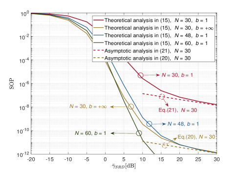
Fig. 2 shows the impact of on the SOP when and . We observe that the analytical results in (15) match well with the numerical curves. Monte-Carlo simulations are illustrated for values of the SOP no smaller than due to the limited number of channel realizations simulated. As stated in Case 3, the gap between and in Fig. 2 does appear negligible for high SNRs.
In Fig. 3, we consider a larger to verify the effectiveness of the asymptotic analysis. We plot the SOP for by setting and . As expected, the asymptotic expressions in (20) and (21) are quite tight in the high-SNR regime. Then, we plot the SOP for by setting (i.e., which is equal to ) and (). We see that the setup with provides, in the high-SNR regime, the same SOP as the setup with , which validates the obtained guideline in Remark 3.
VI Conclusion
This paper studied the SOP of an RIS-assisted communication system with discrete phase shifts. The main contribution is to unveil the achievable scaling law of SOP with respect to and . Specifically, the increased number of RIS elements was quantified to compensate the performance loss caused by binary phase shifts.
Appendix A Proof of The Independence of and
By taking into account that the distribution of is symmetric around its mean value, which is equal to zero, we have [25]. Then, the covariance of and is
| (22) |
which indicates that and are uncorrelated RVs.
For large values of , is approximately a complex Gaussian RV by virtue of the CLT, and its real part and imaginary part are jointly Gaussian RVs. Since two uncorrelated Gaussian RVs are independent as well, it follows that and are independent.
Appendix B Proof of Lemma 2
First, we note that and are dependent RVs since and are correlated RVs. Since , the RV can be rewritten as
| (23) |
where and are uniformly distributed in . The RV depends on the phase error at the RIS, and and depend on the positions of the eavesdropper and the legitimate user, respectively. Since the RV is independent of the three RVs , , and and has zero mean, we obtain , and . For large values of , by virtue of the CLT, and then .
Since is a circularly-symmetric Gaussian RV, we have . Thus, is a zero-mean circularly-symmetric complex Gaussian RV as well. This implies that the real and imaginary parts of are uncorrelated and hence independent since they are Gaussian distributed. Also, they have zero means and the same variance.
Appendix C Proof of Remark 1
Since the RV is nonnegative, we obtain
| (24) |
where (h) is obtained by applying the Markov inequality [19], and (i) comes from the fact that and are independent.
Furthermore, is calculated as
| (25) |
where and it is easy to check that is increasing as grows by calculating its first order derivative. It follows
| (26) |
Therefore, (24) is further expressed as
| (27) |
When is large, we finally obtain , which means that holds with high probability.
Appendix D Proof of Lemma 3
By inserting (8) and (12) in (14), the upper bound of the SOP can be rewritten as
| (28) |
The integral is calculated by using the integration by parts method. We have
| (29) |
where is expressed as
| (30) |
, and the last equality is obtained by using [18, Eq. (3.322)], where and . Further, by substituting (30) into (29), is obtained as shown in (16). Analogously, is calculated by replacing in (16) with , which yields the desired result in (17).
Appendix E Proof of Case 3
We apply the Taylor expansion to the SOP in (18). More precisely, around and for small values of , we have
| (31) |
| (32) |
where , , and .
References
- [1] E. Basar, M. Di Renzo, J. De Rosny, M. Debbah, M.-S. Alouini, and R. Zhang, “Wireless communications through reconfigurable intelligent surfaces,” IEEE Access, vol. 7, pp. 116753–116773, Aug. 2019.
- [2] M. Di Renzo et al., “Smart radio environments empowered by reconfigurable intelligent surfaces: How it works, state of research, and the road ahead,” IEEE J. Sel. Areas Commun., vol. 38, no. 11, pp. 2450–2525, Nov. 2020.
- [3] S. Liu, Z. Gao, J. Zhang, M. Di Renzo, and M.-S. Alouini, “Deep denoising neural network assisted compressive channel estimation for mmWave intelligent reflecting surfaces,” IEEE Trans. Veh. Technol., vol. 69, no. 8, pp. 9223–9228, Aug. 2020.
- [4] Z. Wan, Z. Gao, F. Gao, M. Di Renzo, and M.-S. Alouini, “Terahertz massive MIMO with holographic reconfigurable intelligent surfaces,” IEEE Trans. Commun., vol. 69, no. 7, pp. 4732–4750, Jul. 2021.
- [5] W. Shi, W. Xu, X. You, C. Zhao, and K. Wei, “Intelligent reflection enabling technologies for integrated and green Internet-of-Everything beyond 5G: Communication, sensing, and security,” IEEE Wireless Commun., early access. doi: 10.1109/MWC.018.2100717.
- [6] H. Shen, W. Xu, S. Gong, Z. He, and C. Zhao, “Secrecy rate maximization for intelligent reflecting surface assisted multi-antenna communications,” IEEE Commun. Lett., vol. 23, no. 9, pp. 1488–1492, Sept. 2019.
- [7] L. Dong, H.-M. Wang, J. Bai, and H. Xiao, “Double intelligent reflecting surface for secure transmission with inter-surface signal reflection,” IEEE Trans. Veh. Technol., vol. 70, no. 3, pp. 2912–2916, Mar. 2021.
- [8] G. Zhou, C. Pan, H. Ren, K. Wang, and Z. Peng, “Secure wireless communication in RIS-aided MISO system with hardware impairments,” IEEE Wireless Commun. Lett., vol. 10, no. 6, pp. 1309–1313, Jun. 2021.
- [9] L. Lv, Q. Wu, Z. Li, N. Al-Dhahir, and J. Chen, “Secure two-way communications via intelligent reflecting surfaces,” IEEE Commun. Lett., vol. 25, no. 3, pp. 744–748, Mar. 2021.
- [10] J. Luo, F. Wang, S. Wang, H. Wang, and D. Wang, “Reconfigurable intelligent surface: Reflection design against passive eavesdropping,” IEEE Trans. Wireless Commun., vol. 20, no. 5, pp. 3350–3364, May 2021.
- [11] L. Yang, J. Yang, W. Xie, M. O. Hasna, T. Tsiftsis, and M. Di Renzo, “Secrecy performance analysis of RIS-aided wireless communication systems,” IEEE Trans. Veh. Technol., vol. 69, no. 10, pp. 12296–12300, Oct. 2020.
- [12] W. Wang, H. Tian, and W. Ni, “Secrecy performance analysis of IRS-aided UAV relay system,” IEEE Wireless Commun. Lett., vol. 10, no. 12, pp. 2693–2697, Dec. 2021.
- [13] M. H. Khoshafa, T. M. N. Ngatched, and M. H. Ahmed, “Reconfigurable intelligent surfaces-aided physical layer security enhancement in D2D underlay communications,” IEEE Commun. Lett., vol. 25, no. 5, pp. 1443–1447, May 2021.
- [14] Q. Wu and R. Zhang, “Beamforming optimization for wireless network aided by intelligent reflecting surface with discrete phase shifts,” IEEE Trans. Commun., vol. 68, no. 3, pp. 1838–1851, Mar. 2020.
- [15] A. Papazafeiropoulos, C. Pan, P. Kourtessis, S. Chatzinotas, and J. M. Senior, “Intelligent reflecting surface-assisted MU-MISO systems with imperfect hardware: Channel estimation and beamforming design,” IEEE Trans. Wireless Commun., vol. 21, no. 3, pp. 2077–2092, Mar. 2022.
- [16] H. Zhang, B. Di, L. Song, and Z. Han, “Reconfigurable intelligent surfaces assisted communications with limited phase shifts: How many phase shifts are enough?,” IEEE Trans. Veh. Technol., vol. 69, no. 4, pp. 4498–4502, Apr. 2020.
- [17] P. Xu, G. Chen, Z. Yang, and M. Di Renzo, “Reconfigurable intelligent surfaces-assisted communications with discrete phase shifts: How many quantization levels are required to achieve full diversity?,” IEEE Wireless Commun. Lett., vol. 10, no. 2, pp. 358–362, Feb. 2021.
- [18] I. S. Gradshteyn and I. M. Ryzhik, Table of Integrals, Series, and Products, 7th ed. San Diego, CA, USA: Academic, 2007.
- [19] H. Pishro-Nik, Introduction to Probability, Statistics and Random Processes, Gaithersburg, MD, USA: Kappa Research, 2014.
- [20] J. G. Proakis and M. Salehi, Digital Communications, 5th ed., New York, NY, USA: McGraw-Hill, 2008.
- [21] V. M. Kapinas, S. K. Mihos, and G. K. Karagiannidis, “On the monotonicity of the generalized Marcum and Nuttall Q-functions,” IEEE Trans. Inf. Theory, vol. 55, no. 8, pp. 3701–3710, Aug. 2009.
- [22] M. Elkashlan, L. Wang, T. Q. Duong, G. K. Karagiannidis, and A. Nallanathan, “On the security of cognitive radio networks,” IEEE Trans. Veh. Technol., vol. 64, no. 8, pp. 3790–3795, Aug. 2015.
- [23] N. Wang, P. Wang, A. Alipour-Fanid, L. Jiao, and K. Zeng, “Physical-layer security of 5G wireless networks for IoT: Challenges and opportunities,” IEEE Internet Things J., vol. 6, no. 5, pp. 8169–8181, Oct. 2019.
- [24] S. Zeng, H. Zhang, B. Di, Z. Han, and L. Song, “Reconfigurable intelligent surface (RIS) assisted wireless coverage extension: RIS orientation and location optimization,” IEEE Commun. Lett., vol. 25, no. 1, pp. 269–273, Jan. 2021.
- [25] I. Trigui, W. Ajib, W.-P. Zhu, and M. Di Renzo, “Performance evaluation and diversity analysis of RIS-assisted communications over generalized fading channels in the presence of phase noise,” IEEE Open J. Commun. Soc., vol. 3, pp. 593–607, 2022.