Secure list decoding and its application to bit-string commitment

Relaxing the condition of the decoding process, Elias [1] and Wozencraft [2] independently introduced list decoding as the method to allow more than one element as candidates of the message sent by the encoder at the decoder. When one of these elements coincides with the true message, the decoding is regarded as successful. The paper [3] discussed its algorithmic aspect. In this formulation, Nishimura [4] obtained the channel capacity by showing its strong converse part¹¹1The strong converse part is the argument that the average error goes to $1$ if the code has a transmission rate over the capacity.. That is, he showed that the transmission rate is less than the conventional capacity plus the rate of the list size, i.e., the number of list elements. Then, the reliable transmission rate does not increase even when list decoding is allowed if the list size does not increase exponentially. In the non-exponential case, these results were generalized by Ahlswede [5]. Further, the paper [6] showed that the upper bound of capacity by Nishimura can be attained even if the list size increases exponentially. When the number of lists is $\mathsf{L}$, the capacity can be achieved by choosing the same codeword for $\mathsf{L}$ distinct messages.

However, the merit of the increase in the list size was not discussed sufficiently. To get a merit of list coding, we need a code construction that is essentially different from conventional coding. Since the above capacity-achieving code construction does not have an essential difference from the conventional coding, we need to rule out the above type of construction of list coding. That is, to extract a merit of list decoding, we need additional parameters to characterize the difference from the conventional code construction, which can be expected to rule out such a trivial construction.

To seek a merit of list decoding, we focus on bit commitment, which is a fundamental task in information security. It is known that bit commitment can be realized when a noisy channel is available [7]. Winter et al [8, 9] studied bit-string commitment, the bit string version of bit commitment when an unlimited bidirectional noiseless channel is available between Alice and Bob, and a discrete memoryless noisy channel $W:{\cal X}\to{\cal Y}$ from Alice to Bob, which may be used $n$ times. They derived the asymptotically optimal rate as $n$ goes to infinity, which is called the commitment capacity. Since their result is based on Shannon theory, the tightness of their result shows the strong advantage of Shannon theoretic approach to information theoretic security. This result was extended to the formulation with multiplex coding [10]. However, their optimal method has the following problems;

(P1)

When the number of use of the channel is limited, it is impossible to send a message with a larger rate than the commitment capacity.

(P2)

Their protocol assumes that the output system ${\cal Y}$ is a finite set because they employ the method of type. However, when a noisy channel is realized by wireless communication, like an additive white Gaussian noise (AWGN) channel, the output system ${\cal Y}$ is a continuous set.

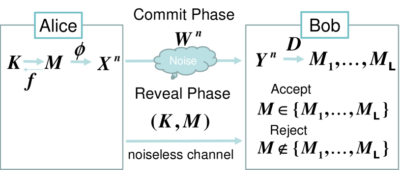
To resolve the problem (P1), it is natural to relax the condition for bit-string commitment. Winter et al [8, 9] imposed strong security for the concealing condition. However, studies in information theory, in particular, papers for wire-tap channel, often employs equivocation rate instead of strong security. In this paper, to relax the condition of bit-string commitment by using equivocation rate, we consider the following simple protocol by employing list decoding, where Alice wants to send her message $M\in\{1,\ldots,\mathsf{M}\}$ to Bob.

(i)

(Commit Phase) Alice sends her message $M$ to Bob via a noisy channel. Bob outputs $\mathsf{L}$ messages as the list. The list is required to contain the message $M$.

(ii)

(Reveal Phase) Alice sends her message $M$ to Bob via a noiseless channel. If $M$ is contained in Bob’s decoded list, Bob accepts it. Otherwise, Bob rejects it.

In order that the protocol with phase (i) and (ii) works for bit-string commitment, the following requirements need to be satisfied.

(a)

The message $M$ needs to be one of $\mathsf{L}$ messages $M_{1},\ldots,M_{\mathsf{L}}$ output by Bob.

(b)

Bob cannot identify the message $M$ at the phase (i).

(c)

Alice cannot find another element among $\mathsf{L}$ messages $M_{1},\ldots,M_{\mathsf{L}}$ output by Bob.

The requirement (a) is the condition for the requirement for the conventional list decoding while the requirements (b) and (c) correspond to the concealing condition and the binding condition, respectively and have not been considered in the conventional list decoding.

In this paper, we propose a new concept of secure list decoding by adding the requirements (b) and (c). One typical condition for (b) is the conventional equivocation rate based on the conditional entropy. In this paper, we also consider the equivocation rate based on the conditional Rényi entropy similar to the paper [11, 12]²²2 While the conference paper [13] discussed a similar modification of list decoding, it did not consider the equivocation rate. In this sense, the content of this paper is different from that of [13].. Hence, our code can be evaluated by three parameters. The first one is the rate of the message size, the second one is the rate of list size, and the third one is the equivocation rate. Using three parameters, we define the capacity region. In addition, our method works with a general output system including a continuous output system, which resolves the problem (P2) while an extension to such a general case was mentioned as an open problem in [9].

In the second step, we extend our result to the case with a general input system including a continuous input system. We need to be careful in formulating the problem setting in this case. If Alice is allowed to access infinitely many input elements in a continuous input system, the conditional entropy rate $H(X|Y)$ might be infinity. Further, it is not realistic for Alice to access infinitely many input elements. because a realistic modulator converts messages to finite constellation points in a continuous input system in wireless communication. Therefore, we need to separately formulate honest Alice and dishonest Alice as follows. The honest Alice is assumed to access only a fixed finite subset of a general input system. But, the dishonest Alice is assumed to access all elements of the general input system. Under this problem setting, we derived the capacity region.

In the third step, we propose a conversion method to make a protocol for bit-string commitment with strong security as the concealing condition (b) by converting a secure list decoding code. In this converted protocol, the security parameter for the concealing condition (b) is evaluated by variational distance in the same way as Winter et al [8, 9]. In particular, this converted protocol has strong security even with continuous input and output systems, where the honest Alice and the dishonest Alice has different accessibility to the continuous input system. In this converted protocol, the rate of message size of the bit-string commitment is the same as the equivocation rate based on the conditional entropy of the original secure list decoding code, which shows the merit of the equivocation rate of a secure list decoding code. In fact, the bit-string commitment with the continuous case was treated as an open problem in the preceding studies [9]. In addition, due to the above second step, our protocol for bit-string commitment works even when the accessible alphabet by the honest Alice is different from the accessible alphabet by the dishonest Alice.

This paper is structured as follows. Section II reviews the existing results for bit-string commitment. Section III explains how we mathematically handle a general probability space as input and output systems including continuous systems. Section IV gives the formulation of secure list decoding. Section V introduces information quantities used in our main results. Section VI states our results for secure list decoding with a discrete input system. Section VII explains our formulation of secure list decoding with general input system and states our results under this setting. Section VIII presents the application of secure list decoding to the bit-string commitment with strong security. Section IX shows the converse part, and Section X proves the direct part.

Before stating our result, we review existing results for bit-string commitment [8, 9]. Throughout this paper, the base of the logarithm is chosen to be $2$. Also, we employ the standard notation for probability theory, in which, upper case letters denote random variables and the corresponding lower case letters denote their realizations. Bit-string commitment has two security parameters, the concealing parameter $\delta_{\mathop{\rm CON}}>0$ and the binding parameter $\delta_{\mathop{\rm BIN}}>0$. We denote the message revealed by Alice in Reveal Phase by $\hat{M}$. Let $Z_{1}$ be all information that Bob obtains during Commit Phase, and $Z_{2}$ be all information that Bob obtains during Reveal Phase except for $\hat{M}$. Here, $Z_{1}$ contains the information generated by Bob. After Reveal Phase, Bob makes his decision, $\mathop{\rm ACC}$ (accept) or $\mathop{\rm REJ}$ (rejection). For this decision, Bob has a function $\beta(Z_{1},Z_{2},\hat{M})$ that takes the value $\mathop{\rm ACC}$ or $\mathop{\rm REJ}$. When Alice intends to send message $M$ in ${\cal M}$ to Bob, the concealing and binding conditions are given as follows.

(CON)

Concealing condition with $\delta_{\mathop{\rm CON}}>0$. When Alice is honest, the inequality

$\displaystyle\frac{1}{2}\|P_{Z_{1}|M=m}-P_{Z_{1}|M=m^{\prime}}\|_{1}\leq\delta_{\mathop{\rm CON}}$

(1)

holds for $m\neq m^{\prime}\in{\cal M}$.

(BIN)

Binding condition with $\delta_{\mathop{\rm BIN}}>0$. We assume that the message $M$ is subject to the uniform distribution on ${\cal M}$. When Alice and Bob are honest,

$\displaystyle{\rm Pr}(\beta(Z_{1},Z_{2},{M})=\mathop{\rm ACC})\geq 1-\delta_{\mathop{\rm BIN}}.$

(2)

When Bob is honest, the inequality

		$\displaystyle{\rm Pr}(\beta(Z_{1},z_{2},m)=\mathop{\rm ACC},\beta(Z_{1},z_{2}^{\prime},m^{\prime})=\mathop{\rm ACC})$
	$\displaystyle\leq$	$\displaystyle\delta_{\mathop{\rm BIN}}$		(3)

holds for $m\neq m^{\prime}\in{\cal M}$ and $z_{2},z_{2}^{\prime}$.

When the protocol with (i) and (ii) is used for bit-string commitment, the conditions (a) and (c) guarantee (2) and (3) of (BIN), respectively, and the condition (b) guarantees (CON).

Now, we denote a noisy channel $\bm{W}$ from a finite set ${\cal X}$ to a finite set ${\cal Y}$ by using a set $\{W_{x}\}_{x\in{\cal X}}$ of distributions on ${\cal Y}$. Winter et al [8, 9] considered the situation that Alice and Bob use the channel $\bm{W}$ at $n$ times and the noiseless channel can be used freely. Winter et al [8, 9] defined the commitment capacity as the maximum rate when the code satisfies Concealing condition with $\delta_{\mathop{\rm CON},n}$ and Binding condition with $\delta_{\mathop{\rm BIN},n}$ under the condition that the parameters $\delta_{\mathop{\rm CON},n}$ and $\delta_{\mathop{\rm BIN},n}$ approach to zero as $n$ goes to infinity. They derived the commitment capacity under the following conditions for the channel $\bm{W}$;

(W1)

${\cal X}$ and ${\cal Y}$ are finite sets.

(W2)

For any $x\in{\cal X}$, the relation

$\displaystyle\min_{x\in{\cal X}}\min_{P\in{\cal P}({\cal X}\setminus\{x\})}D\bigg{(}\sum_{x^{\prime}\in{\cal X}\setminus\{x\}}P(x^{\prime})W_{x^{\prime}}\bigg{\|}W_{x}\bigg{)}>0$

(4)

holds, where $D(P\|Q)$ is the Kullback-Leibler divergence between two distributions $P$ and $Q$. This condition is called the non-redundant condition.

To state their result, we introduce a notation; Given a joint distribution $P_{X,Y}$ on a discrete set ${\cal X}\times{\cal Y}$, we denote the conditional distribution $P_{X|Y=y}$ under the condition that $Y=y$. Then, the conditional entropy $H(X|Y)$ is given as

When the joint distribution $P_{X,Y}$ is given as $P_{X,Y}(x,y)=W_{x}(y)P(x)$ by using a distribution $P\in{\cal P}({\cal X})$, we denote the conditional entropy $H(X|Y)_{P_{X,Y}}$ by $H(X|Y)_{P}$. They showed the following proposition;

Many noisy channels are physically realized by wireless communication, and such channels have continuous output system ${\cal Y}$. Indeed, if we apply discretization to a continuous output system ${\cal Y}$, we obtain a discrete output system ${\cal Y}^{\prime}$. When we apply their result to the channel with the discrete output system ${\cal Y}^{\prime}$, the obtained protocol satisfies Condition (BIN) even when Bob uses the continuous output system ${\cal Y}$. However, the obtained protocol does not satisfy Condition (CON) in general under the continuous output system ${\cal Y}$.

In fact, Condition (W2) can be removed and Proposition 1 can be generalized as follows. Therefore, Condition (W2) can be considered as an assumption for simplifying our analysis.

Proposition 2 follows from Proposition 1 in the following way. Due to Condition (W1), the channel $\bm{W}$ with input alphabet ${\cal X}_{0}$ satisfies Condition (W2) as well as (W1). Hence, the commitment capacity is lower bounded by (9). Since any operation with the channel $\bm{W}$ with input alphabet ${\cal X}$ can be simulated with ${\cal X}_{0}$. Therefore, the commitment capacity is upper bounded by (9). Thus, we obtain Proposition 2.

We focus on an input alphabet ${\cal X}$ with finite cardinality, and denote the set of probability distributions on ${\cal X}$ by ${\cal P}({\cal X})$. But, an output alphabet ${\cal Y}$ may have infinite cardinality and is a general measurable set. In this paper, the output alphabet ${\cal Y}$ is treated as a general probability space with a measure $\mu(dy)$ because this description covers the probability space of finite elements and the set of real values. Hence, when the alphabet ${\cal Y}$ is a discrete set including a finite set, the measure $\mu(dy)$ is chosen to be the counting measure. When the alphabet ${\cal Y}$ is a vector space over the real numbers $\mathbb{R}$, the measure $\mu(dy)$ is chosen to be the Lebesgue measure. Throughout this paper, we will use an upper case letter and corresponding lower case letter to stand for a probability measure and its density function. When we treat a probability distribution $P$ on the alphabet ${\cal Y}$, it is restricted to a distribution absolutely continuous with respect to $\mu(dy)$. In the following, we use the lower case $p(y)$ to express the Radon-Nikodym derivative of $P$ with respect to the measure $\mu(dy)$, i.e., the probability density function of $P$ so that $P(dy)=p(y)\mu(dy)$. This kind of channel description covers many useful channels. For example, phase-shift keying (PSK) scheme of additive white Gaussian noise (AWGN) channels satisfies this condition. In addition, the capacity of AWGN channel with the energy constraint can be approximately achieved when the input alphabet for encoding is restricted to a finite subset of the set of real numbers.

For a distribution $P$ on ${\cal Y}$ and a general measure $Q$ on ${\cal Y}$, we define the Kullback–Leibler (KL) divergence $D(P\|Q):=\mathbb{E}_{P}[\log\frac{p(Y)}{q(Y)}]$ and Rényi divergence of order $\alpha(\neq 1)>0$ $D_{\alpha}(P\|Q):=\frac{1}{\alpha-1}\log\mathbb{E}_{P}[(\frac{p(Y)}{q(Y)})^{\alpha-1}]$.

When ${\cal M}$ is a finite set and ${\cal Y}$ is a general probability space, the conditional entropy is defined as

This quantity can be written as

where $I_{M}$ is defined as $I_{M}(m)=1$. We focus on the following type of Rényi conditional entropy $H_{\alpha}(M|Y)$ as [14, 15, 16]

$H_{\alpha}(M|Y)$ is monotonically decreasing for $\alpha$ [16, Lemma 7]. Hence, we have $H(M|Y)\geq H_{\alpha}(M|Y)$ for $\alpha>1$. It is known that the maximum is attained by $q_{\alpha}(y):=\frac{(\sum_{m}p_{MY}(m,y)^{\alpha})^{1/\alpha}}{\int_{{\cal Y}}(\sum_{m}p_{MY}(m,y)^{\alpha})^{1/\alpha}\mu(dy)}$ [16, Lemma 4]. Hence, when two pairs of variables $(M_{1},Y_{1})$ and $(M_{2},Y_{2})$ are independent, we have the additivity;

References

• [1] P. Elias, “List decoding for noisy channels,” in WESCON Conv. Rec., 1957, pp. 94- 104.
• [2] J.M. Wozencraft, “List decoding,” Quart. Progr. Rep. Res. Lab. Electron., MIT, Cambridge, MA Vol. 48, 1958.
• [3] V. Guruswami, “Algorithmic results in list decoding,” Foundations and Trends in Theoretical Computer Science, Vol. 2, No. 2, 107–195 (2007).
• [4] S. Nishimura. “The strong converse theorem in the decoding scheme of list size LL,” Kōdai Math. Sem. Rep., 21, 418–25, (1969).
• [5] R. Ahlswede, “Channel capacities for list codes,” J. Appl. Probab., vol. 10, 824–836, 1973.
• [6] M. Hayashi, “Channel capacities of classical and quantum list decoding,” arXiv:quant-ph/0603031.
• [7] C. Crépeau, “Efficient Cryptographic Protocols Based on Noisy Channels,” Advances in Cryptology: Proc. EUROCRYPT 1997 , pp. 306–317, Springer 1997.
• [8] A. Winter, A. C. A. Nascimento, and H. Imai, “Commitment Capacity of Discrete Memoryless Channels,” Proc. 9th IMA International Conferenece on Cryptography and Coding (Cirencester 16-18 December 2003), pp. 35-51, 2003.
• [9] H. Imai, K. Morozov, A. C. A. Nascimento, and A. Winter, “Efficient Protocols Achieving the Commitment Capacity of Noisy Correlations,” Proc. IEEE ISIT 2006, pp. 1432-1436, July 6-14, 2006.
• [10] H. Yamamoto and D. Isami, “Multiplex Coding of Bit Commitment Based on a Discrete Memoryless Channel,” Proc. IEEE ISIT 2007, pp. 721-725, June 24-29, 2007.
• [11] V. Y. F. Tan and M. Hayashi, “Analysis of remaining uncertainties and exponents under various conditional Rényi entropies,” IEEE Transactions on Information Theory, Volume 64, Issue 5, 3734 – 3755 (2018).
• [12] L. Yu and V. Y. F. Tan, “Rényi Resolvability and Its Applications to the Wiretap Channel,” IEEE Transactions on Information Theory, Volume 65, Issue 3, 1862 – 1897 (2019).
• [13] M. Hayashi, “Secure list decoding” Proc. IEEE International Symposium on Information Theory (ISIT2019), Paris, France, July 7 – 12, 2019, pp. 1727 – 1731; https://arxiv.org/abs/1901.02590.
• [14] S. Arimoto, “Information measures and capacity of order α\alpha for discrete memoryless channels,” Colloquia Mathematica Societatis János Bolyai, 16. Topics in Information Theory 41–52 (1975)
• [15] M. Iwamoto and J. Shikata, “Information theoretic security for encryption based on conditional Rényi entropies,” Information Theoretic Security (Lecture Notes in Computer Science), vol. 8317. Berlin, Germany: Springer, 2014, pp. 103–121.
• [16] M. Hayashi, “Security analysis of epsilon-almost dual universal2 hash functions: smoothing of min entropy vs. smoothing of Renyi entropy of order 2,” IEEE Trans. Inform. Theory, 62(6) 3451 – 3476 (2016).
• [17] I. Csiszár and J. Körner, “Broadcast channels with confidential messages,” IEEE Trans. Inform. Theory, 24(3) 339 – 348 (1978).
• [18] R. Sibson, “Information radius,” Z. Wahrscheinlichkeitstheorie und Verw. Geb., vol. 14, pp. 149–161, 1969.
• [19] L. Carter and M. Wegman, “Universal classes of hash functions,” J. Comput. System Sci., vol. 18(2), 143–154 (1979).
• [20] M. N. Wegman and J. L. Carter, “New Hash Functions and Their Use in Authentication and Set Inequality,” J. Comput. System Sci., 22, 265-279 (1981).
• [21] M. Hayashi, “Tight exponential analysis of universally composable privacy amplification and its applications,” IEEE Trans. Inform. Theory, 59(11) 7728 – 7746 (2013).
• [22] M. Hayashi and S. Watanabe, “Uniform Random Number Generation from Markov Chains: Non-Asymptotic and Asymptotic Analyses,” IEEE Trans. Inform. Theory, 62(4) 1795 – 1822 (2016).
• [23] S. Verdú and T. S. Han, “A general formula for channel capacity,” IEEE Trans. Inform. Theory, 40(6) 1147–1157, (1994).
• [24] M. Hayashi and H. Nagaoka, “General formulas for capacity of classical-quantum channels,” IEEE Trans. Inform. Theory, 49(7), 1753–1768 (2003).
• [25] A. C. A. Nascimento, J. Barros, S. Skludarek and H. Imai, “The Commitment Capacity of the Gaussian Channel Is Infinite,” IEEE Trans. Inform. Theory, 54(6), 2785 – 2789 (2008).
• [26] T. M. Cover and J. A. Thomas, Elements of Information Theory: Second Edition, New York Wiley-Interscience (2006).
Masahito Hayashi (Fellow, IEEE) was born in Japan in 1971. He received the B.S. degree from the Faculty of Sciences in Kyoto University, Japan, in 1994 and the M.S. and Ph.D. degrees in Mathematics from Kyoto University, Japan, in 1996 and 1999, respectively. He worked in Kyoto University as a Research Fellow of the Japan Society of the Promotion of Science (JSPS) from 1998 to 2000, and worked in the Laboratory for Mathematical Neuroscience, Brain Science Institute, RIKEN from 2000 to 2003, and worked in ERATO Quantum Computation and Information Project, Japan Science and Technology Agency (JST) as the Research Head from 2000 to 2006. He worked in the Graduate School of Information Sciences, Tohoku University as Associate Professor from 2007 to 2012. In 2012, he joined the Graduate School of Mathematics, Nagoya University as Professor. In 2020, he joined Shenzhen Institute for Quantum Science and Engineering, Southern University of Science and Technology, Shenzhen, China as Chief Research Scientist. In 2011, he received Information Theory Society Paper Award (2011) for “Information-Spectrum Approach to Second-Order Coding Rate in Channel Coding”. In 2016, he received the Japan Academy Medal from the Japan Academy and the JSPS Prize from Japan Society for the Promotion of Science. In 2006, he published the book “Quantum Information: An Introduction” from Springer, whose revised version was published as “Quantum Information Theory: Mathematical Foundation” from Graduate Texts in Physics, Springer in 2016. In 2016, he published other two books “Group Representation for Quantum Theory” and “A Group Theoretic Approach to Quantum Information” from Springer. He is on the Editorial Board of International Journal of Quantum Information and International Journal On Advances in Security. His research interests include classical and quantum information theory and classical and quantum statistical inference.