Secure distributed adaptive optimal coordination of nonlinear cyber-physical systems with attack diagnosis
Abstract
This paper studies the problem of distributed optimal coordination (DOC) for a class of nonlinear large-scale cyber-physical systems (CPSs) in the presence of cyber attacks. A secure DOC architecture with attack diagnosis is proposed that guarantees the attack-free subsystems to achieve the output consensus which minimizes the sum of their objective functions, while the attacked subsystems converge to preset secure states. A two-layer DOC structure is established with emphasis on the interactions between cyber and physical layers, where a command-driven control law is designed that generates provable optimal output consensus. Differing from the existing fault diagnosis methods which are generally applicable to given failure types, the focus of the attack diagnosis is to achieve detection and isolation for arbitrary malicious behaviors. To this end, double coupling residuals are generated by a carefully-designed distributed filter. The adaptive thresholds with prescribed performance are designed to enhance the detectability and isolability. It is theoretically guaranteed that any attack signal cannot bypass the designed attack diagnosis methodology to destroy the convergence of the DOC algorithm, and the locally-occurring detectable attack can be isolated from the propagating attacks from neighboring subsystems. Simulation results for the motion coordination of multiple remotely operated underwater vehicles illustrate the effectiveness of the proposed architecture.
keywords:
Cyber-physical systems, distributed optimization, attack diagnosis, nonlinear systems, adaptive control.,
1 Introduction
Recently, Cyber-Physical Systems (CPSs), which closely connect cyber and physical worlds, have gained much research interest in many fields, such as computer field, control field, battle field. By utilizing the close interaction between cyber and physical parts, the “intelligence” of physical systems can be sufficiently enhanced in order to fulfil some complex, precise or dangerous tasks, such as remote diagnosis, deep sea exploration [1]. However, the networked connection between cyber and physical parts also often leads to large attack space, such that the CPSs are vulnerable to various types of adversarial attacks. Some famous examples such as the Maroochy water breach [2] and Stuxnet [3] indicate the CPS security as a fundamental issue to be studied.
With potential applications of distributed optimization in large-scale CPSs [21], many important results on discrete- or continuous-time DO algorithms have been reported [4, 5, 6, 7, 8]. In these algorithms, each individual (or said agent in multi-agent systems) only performs the designed optimization dynamics, ignoring its own dynamics. Note that the physical dynamic systems are usually indispensable parts for achieving DO task, such as the cooperative search of radio sources [9], the motion coordination [14] and the distributed optimal power flow [10, 11]. Hence, it is relevant to study the distributed optimization problems together with physical dynamics, termed distributed optimal coordination (DOC). In fact, the DOC can be completed based on the CPS architecture by effectively combining of cyber computation/communication and physical dynamics/control [12]. Recently, many important results for DOC have been reported for multi-agent system with various physical dynamics by designing integrated closed-loop control laws, such as integrator-type dynamics [13, 14, 15], continuous-time linear dynamics [16, 17], Euler-Lagrangian dynamics [12]. More references for DOC can be found in [18]. Motivated by these and considering the non-ignorable nonlinear uncertain dynamics in many physical agents [40, 41, 12], this paper investigates the DOC problem for a class of certain nonlinear large-scale systems on the CPS platforms.
Given the growing threat of malicious attacks in large-scale (and safety-critical) CPSs, the vulnerability of consensus-based DOC algorithms is also with respect to cyber attacks. Hence, the other main objective of this paper is to address the issue of security of consensus-based DOC dynamics by providing certain safety guarantees based on attack diagnosis. The recent works [20, 21, 22] also consider the problem of resilient DO under different adversarial models than the ones that we consider here, and the agent’s own physical dynamics is not considered there. Other related important works on distributed/decentralized sensor fault diagnosis and secure state estimation against sensor attacks for large-scale CPSs have been reported in [24, 25, 26, 27, 28, 29, 30]. In the existing fault diagnosis and fault-tolerant results, the fault detectors are in general designed for given failure types [42, 43], such as loss of effectiveness [27], bias faults [24, 25, 26]. As we will see later, in our problem formulation the attack model can be considered to contain infinite number of failure types and one cannot afford to construct a fault detector for each possible failure type. In [28, 29, 30], the attack-resilient mechanisms are designed in the presence of arbitrary adversarial behaviors under the framework of distributed estimation, outside of DOC framework.
In this paper, we propose a secure DOC architecture for a class of nonlinear large-scale CPSs in the presence of cyber attacks. The overall architecture consists of cyber and physical parts, and each physical subsystem is modeled as a nonlinear parametric strict-feedback system equipped with a dedicated decision-making agent in the cyber superstratum. The cyber core (multi-agent network) focuses on the design of DOC and attack diagnosis, and the physical part performs the corresponding optimization task following the cyber-core control command. The objective is to steer the physical systems to achieve the output consensus at the minimizer of a given team performance function in a distributed fashion and provide certain safety guarantees based on attack diagnosis. The contributions of this paper are threefold.
The first contribution of this paper is, differing from the existing integrated closed-loop control schemes proposed in [12, 13, 14, 15, 16, 17], to propose a two-layer DOC structure where the cyber-layer optimizer generates a control command which is transmitted to the physical-layer control for local regulation. To overcome the difficulty caused by the dynamic mismatch between the traditional DO algorithms [4, 5, 6, 7, 8] and adaptive backstepping control systems [36, 37, 38, 39], a novel command-driven control strategy is designed. It is proved that the proposed algorithm ensures all subsystems to achieve the optimal consensus under the healthy (attack-free) environment.
As the second contribution, we provide the design and analysis of an attack detection and isolation (ADI) methodology. The existing fault diagnosis schemes are usually designed for given fault types [42, 43] and cannot guarantee the detectability for arbitrary malicious behaviors in theory. Also, due to the coupling effects of multiple propagated attacks on the physical dynamics and cyber dynamics which are interacted, the attack isolation becomes more challenging. To this end, double coupling residuals and analytical redundancy relations (ARRs) are generated by a carefully-designed distributed filter. The adaptive thresholds with prescribed performance are designed to enhance the detectability and isolability. It is theoretically guaranteed that any attack signal cannot bypass the ADI methodology to destroy the convergence of the DOC algorithm, and the locally-occurring detectable attacks can be isolated from the propagating attacks from the neighboring subsystems.
The last contribution is to develop a secure version of the DOC protocol based on the ADI methodology, which can provide a safety guarantee in the sense that the healthy physical subsystems (satisfying ARRs) reach the output consensus at the optimal solution of the sum of their objective functions, while the attacked physical subsystems (not satisfying ARRs) converge to preset secure states.
2 Preliminaries
2.1 Notations
The symbols and denote the set of real and Boolean numbers, respectively. represents the set of -order differentiable -dimension function vectors. The cardinality of a set is denoted by . and stand for the Kronecker product and Hadamard product, respectively. For a given time interval , represents its Lebesgue measure. represents the sign function. Denote . For a vector sequence , we denote the notation if not specified.
2.2 Graph theory
A weighted undirected graph consists of vertices (or nodes, or agents in multi-agent networks) , a set of edges (or links) and an adjacency matrix with nonnegative element if and otherwise. The neighbors of vertex are denoted by the set . The Laplacian matrix associated with graph is defined as and for . For an undirected graph, the matrix is symmetric and semi-positive. A path from vertex to vertex in graph is a sequence of edges in the graph with distinct nodes . An undirected graph is connected if there is a path from every vertex to other vertex in the graph.
3 DOC architecture
Consider a CPS consisting of subsystems, which aims at achieving the DOC task. The th subsystem, is described by the pair , where denotes the cyber part which is responsible for task decision-making, while denotes the physical part which is responsible for task execution. The physical part is modeled as a nonlinear dynamical system
| (1) |
where , , , is the measurable state; is the control input; and are known nonsingular matrix; is unknown constant; is the output measurement transmitted to the cyber superstratum through a wireless network channel and denotes the cyber attacks corrupting the sensor transmitting signal. In particular, in order to provide security guarantees against worst case adversarial behavior, we allow the adversarial attacker to know the overall system model, system state, control input and the possible fault detector (e.g., distributed adaptive observers [24, 25, 26]) equipped on the CPS. Thus, the attack signal can be modeled as
where is the time profile and is an unknown function that occurs at the unknown time instant . We make no assumption on , which may be any (such as unbounded, discontinuous) function vector. The time profile of the attack is modeled as if and otherwise. Multiple cyber attacks may occur simultaneously or sequentially, for example, with .
Remark 1. System (1) can represent many practical systems such as mobile robots, chemical reactors, wind tunnels, and autonomous vehicles [36]. Some extensive researches for system (1) in presence of external disturbances, actuator failures, etc., have been studied well [37, 38, 39] (these are easily extended to the current framework and thus no longer considered here). Particularly, the works in [40, 41] investigated the adaptive leader-following consensus control of system (1). In this paper, the problem of DOC further minimizes a given team performance function on the basis of consensus.
Remark 2. In general, the fault detector is designed for given failure types and cannot guarantee the detectability for arbitrary malicious behaviors in theory. Due to adversary’s strategic design, here we can assume that the attack signal in system (1) denotes a strategic attack model which can potentially bypass the fault detector to destroy the system convergence based on the knowledge of system and detector (see stealthy attack design methods against various fault detectors, e.g., [32, 33, 34, 35] and references therein).
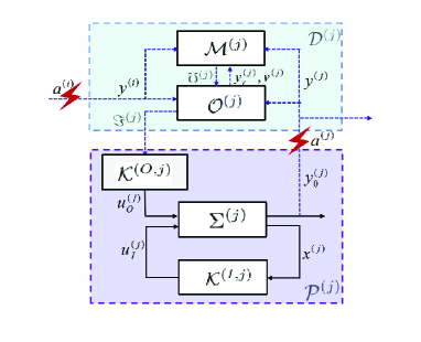
The overall DOC architecture of the considered CPS is illustrated in Fig. 1. Similar CPS architectures can also be found in [31, 26]. The cyber part consists of a decision-making multi-agent network. Each decision-making agent, denoted by , is responsible for sending the control command to . The agent contains an optimization module and a monitoring module, denoted by and , respectively. The module is used to optimize its local objective function, while exchanging its information with its neighbors under a network topology . Since the adversarial attackers can perform the attack to corrupt the communication from physical stratum to cyber stratum, a cyber attack in the subsystem can also be propagated to neighbors via the information exchange between the agent and its neighboring agents. This complicates the identification of attacked subsystems. To address it, each module is used to detect and isolate the cyber attack . In the physical part , the control module consisting of an inner-loop stabilizing module and an outer-loop tracking module drives the physical dynamics in accordance with the control command coming from the decision-making agent . Fig. 1 illustrates that sufficient interaction between cyber and physical parts in the CPS architecture.
Objective of this paper: Design the decision-making agent (including the optimization module and the monitoring module ) and the control agent , such that
1) Optimality: Under the healthy (attack-free) condition, all the physical subsystems cooperatively reach the optimal output that minimizes the following team performance function:
| (2) |
where is a local performance function privately known to the agent ; and all the closed-loop signals of the physical system are uniformly ultimately bounded (UUB).
2) Security: Detect and isolate multiple cyber attacks occurring at the network communication between physical stratum and cyber superstratum, and guarantee that the attacked subsystem , converges to a given secure state , while the healthy subsystems achieve the output consensus at the optimal solution of
| (3) |
where represents the index set of the healthy subsystems, i.e., , and .
Here we consider the scenario that the communication from physical stratum to cyber superstratum can be attacked, while the communication from the cyber superstratum to the physical stratum is secure [35]. For example, for the GPS spoofing attacks on multiple Unmanned Aerial Vehicles (UAVs) [45], the GPS attacker in fact can tamper with the location information transmitted from the UAV to the ground station, but cannot tamper with the control command from the ground station to the UAV or other communications among the ground stations. Indeed, in many practical situations, the adversarial attackers may also tamper with the control command transmitted from cyber superstratum to physical stratum or communication among decision-making agents in the cyber superstratum; however, the design of the attack diagnosis and attack-tolerant strategy is beyond the scope of this paper.
Assumption 1. The function is differentiable and convex for all .
Assumption 2. The graph of the network is undirected and connected.
Remark 3. Assumptions 1 and 2 are common in the DO or DOC literature [8, 12, 13, 14, 15, 16, 17, 21]. In fact, many practical optimization problems can be formalized by the current convex DOC problem or approximated by it using convex relaxation, such as the motion coordination [14], target aggregation [12], search of radio sources [12], optimal power flow [10], and so on. The DOC problems for pure-integrator dynamics [13, 14, 15], Euler-Lagrangian systems [12] and linear time-invariant systems [16, 17] have been studied well. This paper further considers more complex nonlinear case (system (1)). Note that a simple combination of traditional DO algorithms [4, 5, 6, 7, 8] and adaptive backstepping controls [36, 37, 38, 39] will cause the mismatch between (cyber) optimization dynamics and physical dynamics and resultantly cannot guarantee the overall convergence.
Let denote the estimate of agent about the value of the solution to (3) and denote and . Then problem (3) is equivalent to
| (4) |
Since is convex and the constraint in (4) is linear, the constrained optimization problem is feasible. The following lemma gives the analysis on the optimal solution of (4).
Lemma 1 [8]. Under Assumptions 1 and 2, define by
Then is differentiable and convex in its first argument and linear in its second, and:
(i) if is a saddle point of , then is a solution of (4);
(ii) if is a solution of (4), then there exists with such that is a saddle point of .
In what follows, we present the resilient DOC scheme by three steps. First, under the healthy conditions, we provide a basic version of DOC protocol (Section 4); Second, under the adversarial conditions, an ADI methodology is proposed to identify the attacked subsystems (Section 5); Third, the final secure DOC scheme is derived by formulating appropriate ADI-based attack countermeasure strategy for the basic version (Section 6).
Remark 4. In the cyber superstratum, all the decision-making agents themselves are assumed to be healthy in the sense that they will follow any algorithm that we prescribe. However, due to the occurrence of cyber attack , the agent and its neighbors will receive false measurements and thus be induced as “malicious” agents in network topology. Moreover, these agents also send false data to other healthy agents and cause cascading failures [19]. These tamped measurements allow the corrupted agents to update their states to arbitrary values such that the corresponding physical subsystems follow false decision commands. In this paper, a resilient DOC algorithm will be developed, where the corresponding secure countermeasure based on an ADI method can effectively avoid the occurrences of “malicious agents” and cascading failures.
4 Basic DOC under healthy environment
This section deals with the designs of the optimization module and control agent that form a basic DOC scheme under healthy conditions, i.e., for any and . In the sequel, we drop the time argument of the signals for notational brevity.
4.1 DOC control algorithm
The model of the optimization module is designed as the following algorithm
| (5) |
where , and and represent the agent state vectors; is the gradient of and is a design parameter, and is the output that serves as a control command transmitted to the physical subsystem .
Next, we present the design of control agent which consists of inner-loop module and outer-loop module following the control command . First, we define the following changes of coordinates
| (6) |
where is the virtual control function determined at the th step and spitted into two parts: inner-loop control and outer-loop control . Similarly, is the control input consisting of inner-loop control and outer-loop control . They can be respectively expressed as follows:
Inner-loop control
| (7) | |||
| (8) |
The corresponding update laws are given as
| (9) | ||||
| (10) | ||||
| (11) |
where
with being an exponentially decaying function with lower bound such that , and denotes the th () element of ; , for ; and , and are the estimates of with , and , respectively, where is defined in the appendix; is a positive definite matrix and , and for are positive constants, all chosen by users. Here the nonlinear function is introduced to constrain the bound of tracking error , motivated by the prescribed performance technique [39], which will play an important role in enhancing the sensitivity and robustness of the ADI scheme (refer to Remark 7).
Outer-loop control
| (12) | ||||
| (13) | ||||
| (14) |
Algorithm 1: DOC under healthy environment DO algorithm (Module ):
| (15) | ||||
where and . Adaptive tracking control (Module ):
Inner-loop control :
| (16) | ||||
| (17) | ||||
| (18) |
where , , , , , , and
Outer-loop control :
| (19) | ||||
| (20) | ||||
| (21) |
where and . Update laws:
| (22) | ||||
| (23) | ||||
| (24) |
where and .
It can be seen that, the DOC structure consists of two-layer dynamics: the optimization dynamics and the physical dynamics which interact with each other over the communication signals and (see Fig. 1). Such an architecture also illustrates the CPS’s feature that the cyber and physical worlds are integrated. In the inner-loop , a traditional adaptive backstepping controller [36] (i.e., let ) with slight modifications is applied to stabilize the nonlinear strict-feedback system; In the outer-loop , a tracking controller is constructed in order to guarantee that the system output can well track the control command coming from the cyber superstratum. It can be seen that the control laws of the physical systems do not change with the change of the control commands. Summarizing the above procedure (5)-(14), we derive Algorithm 1 for the DOC of the overall CPS under healthy environment.
4.2 Convergence analysis
In the section, we discuss the convergence of the proposed DOC algorithm. The main result is stated in the following theorem whose proof is placed in Appendix I.
Theorem 1. Under Assumptions 1 and 2, the closed-loop CPS with , achieves output consensus at an optimal solution of problem (2), i.e., and all the closed-loop signals are UUB in the absence of cyber attacks if .
Remark 5. Differing from the previous works [12, 13, 14, 15, 16, 17] where the integrated closed-loop control laws are designed, this paper presents a new two-layer control structure based on the traditional DO algorithms [4, 5, 6, 7, 8] and adaptive backstepping controls [36, 37, 38, 39]. Note that the main challenge focuses on how to eliminate the dynamics mismatch between two layers and generate provable optimal consensus. From the proof of Theorem 1 (see (50), (55) and (60)), the dynamics compensation between cyber dynamics and physical dynamics guarantees the convergence of the overall CPS, where the adaptive mechanism (9)–(11) plays a key role.
5 Distributed ADI
This section deals with the design of the monitoring module , . The ADI structure follows the standard one of fault detection and isolation (FDI), formulated by the ARRs of residuals and detection thresholds, e.g., [26, 25]. However, in this section we will focus on achieving the detection and isolation for arbitrary malicious behaviors by constructing new residuals and thresholds. Also, due to the coupling effects of multiple propagated attacks on the physical dynamics and optimization dynamics, the design of attack diagnosis becomes more challenging.
Before giving the main result of this section, we make the following assumption.
Assumption 3. The unknown parameter vector lies in a known bounded convex set
where is a convex function.
Assumption 3 is common in the existing results for fault diagnosis [25, 26, 37], and this is also necessary to detect the attack in transient response phase. It implies that the upper bounds of and , say, , can be obtained, respectively. Noting that depends on the unknown vector , then we define function and , where is the Lyapunov function defined in proof of Theorem 1.
5.1 Design of ADI methodology
The ADI methodology consists of detection filter, adaptive threshold and decision logic. Next, we will give detailed design procedures.
5.1.1 Detection filter and residual generation
Now, we design a distributed filter to generate residuals for detecting attacks. According to the dynamics structure (5) of , the monitoring module is designed as
| (25) |
where and are the estimates of and (even and are available for ), respectively, based on the local communication signals and , . Further, we define two residuals
| (26) | ||||
| (27) |
Taking (5) and (25) into account, the error dynamics can be expressed as
| (28) | ||||
| (29) |
where and .
It is noted that the error dynamics (28)–(29) has a decentralized form where only own information is used in each error dynamics. The feature means that the coupling effects of the propagated attacks on the residuals and caused by the optimization dynamics have been removed such that the locally occurring attack can be isolated. Later, we will further address the coupling effects of the propagated attacks on the residuals caused by the physical dynamics . Moreover, to enhance the attack detectability and remove the existence of stealthy attacks, double coupling residuals have been used here.
If the sensor transmitted information is not affected by local attack , the error dynamics under healthy conditions, denoted by , can be expressed by
| (30) | ||||
| (31) |
The stability of the estimation error dynamics under healthy conditions is analyzed in the following lemma whose proof is placed in Appendix II.
Lemma 2. The residuals under the healthy conditions and satisfy
| (32) | ||||
| (33) |
where .
5.1.2 Construction of adaptive thresholds
The th detection thresholds, denoted by and , are designed based on the bounds of residuals and under the healthy conditions, respectively. It is noted that the right-hand sides of (32) and (33) cannot be directly used as the thresholds because () is unavailable for the modules and due to the existence of cyber attack . To derive an available and reasonable threshold, a heuristic idea is to give a robust design w.r.t. the unknown “disturbance-like” term which, intrinsically, reflects the effects of physical dynamics on the residuals. Hence, we bound the th tracking error under the healthy conditions in the following lemma whose proof is placed in Appendix III.
Lemma 3. Under Assumption 3, the servo tracking error under healthy conditions (i.e., ) satisfies and .
Remark 6. An intuitive method for the ADI design may assess the change of error signal based on Lemma 3, because under the healthy conditions and under cyber attacks. However, we emphasize that the error cannot be directly used as the residual to detect and isolate the cyber attacks because may be simultaneously affected by multiple propagated attacks and the locally occurring attack . The adversarial attacker may cooperatively design the stealthy attacks to degrade the system performance while avoiding detection [32, 33, 34].
Next, we design the detection threshold based on the bound of under the healthy condition. To be specific, from Lemma 3, one has where . Substituting the relation into (32) and (33) yields that
Thus, we define the two adaptive thresholds
where and .
Remark 7. From (28) and (29), multiple propagated attacks have coupling effects on residuals and over the physical dynamics. To address it, in the inner-loop control module the modified prescribed performance technique is used to restrict the bound of tracking error (introduce the nonlinear function into ). As a result, the detection thresholds, or further the proposed ADI method, are robust against the multiple propagated attacks. Especially, the prescribed performance bound constraint is incorporated and contributes to smaller thresholds (from the definition of ) and restrain the coupling effects of propagated attacks on and such that the sensitivity and isolability to the cyber attacks are improved.
5.1.3 Decentralized ADI decision logic
The ADI decision logic implemented in each module is based on the ARR, denoted by , which is defined as
| (34) |
where
If is violated, will generate an alarm.
The decentralized ADI decision logic is formulated by considering the sensitivity w.r.t local cyber attacks and the isolability w.r.t propagated cyber attacks , , which are summarized in the following theorem.
Theorem 2. Consider the ARR defined in (34). The following statements are satisfied:
- a)
-
Attack sensitivity: If there is a time instant when is not satisfied, then the occurrence of the local cyber attack is guaranteed.
- b)
-
Attack isolability: If the transmitted sensor information is not affected by cyber attack , then the ARR is always satisfied even in the presence of the propagated cyber attacks , .
Proof. a) For sake of contradiction, we suppose that no communication attack has occurred, then is always satisfied according to Lemma 2.
b) Under the condition that , even though the propagated cyber attack may exist, , the estimation error dynamics (28)-(29) reduces to (30)-(31), respectively. Then (32) and (33) are valid and, consequently, is always satisfied.
Compared with the existing FDI results [24, 25, 26], we have introduced the following techniques to improve the detectability and isolability for attacks:
-
•
Double coupling residuals are adopted, which will play a key role in removing stealthy attacks (see Lemma 6).
-
•
The modified prescribed performance technique is applied to enhance the sensitivity and isolability to the cyber attacks (See Remark 7).
5.2 Detectability analysis and avoidance of stealthy attacks
In this section, we will evaluate the attack detectability of the proposed ADI methodology. We first give some properties of functions and in the adaptive thresholds, which are important for analyzing the detectability performance of the ADI methodology.
Lemma 4. Let , where , and are positive design parameters such that . Then
(a) ;
(b) ;
(c) , .
Proof. (a) Note that increases as increases. Based on the constraint , we have
By direct computation, the inequality in (a) holds.
(b) Based on (a) and using similar analysis, the proof can be completed.
(c) Let , i.e., . Since is a compact set, satisfies .
To show (c), we construct the auxiliary dynamics
| (35) |
By integrating the dynamics we can find . On the other hand, considering the Lyapunov function , its derivative along with (35) satisfies
integrating two sides of which yields . Using similar procedure to , it is easily obtained that .
From Lemma 4-(c), one has and following Barbalat’s Lemma. It means that only if is satisfied, the bound functions and will converge to zero, which in turn implies that and converge to zero. Lemma 4-(a) and -(b) give prescribed performance bounds of and . By replacing and with the prescribed performance bounds, we can obtain low-complexity thresholds. However, such relaxations will weaken the detectability and extend the detection time. Also, two modified thresholds converge to and instead of zero, which may generate the stealthy attacks. Nevertheless, we can choose to be sufficiently small such that the effects of the stealthy attacks resulted from the relaxation are sufficiently small.
To examine the sensitivity of attacks that can be detectable by the proposed attack detection scheme, the following attack detectability is analyzed.
Lemma 5 (Detectable attacks). The cyber attack occurring at the CPS is detected using the ARR , if there exists some time instant ( is the first time instant of attack occurrence) such that the attack satisfies
| (36) |
or
| (37) |
then the attack is detected at the time .
Proof. After the first occurrence of the attack , i.e., , the time derivative of becomes
Integrating both sides and applying the triangular inequality yield
substituting (36) into which yields
Following the similar analysis, (37) guarantees
From the definition of , the attack satisfying (36) or (37) provokes the violation of ARR and resultantly is detected when .
The inequalities (36)-(37) characterize the class of detectable cyber attacks under the worst-case detectability. The computation of detection time may be somewhat conservative. However, differing from the fault, the attacker may strategically design the (worst-case) attack to extend the detection time as much as possible. Thus, the real-time detection time may sufficiently approach to but not exceed than it. In general, from (36)-(37), if the cyber attack on the time interval is sufficiently large, then the attack can be detected. However, a crafty attacker may ingeniously inject the attack signals which are not detected by the proposed distributed ADI scheme, yet degrade the system performance. The following lemma 6 gives the property of the undetectable attack.
Lemma 6 (Undetectable attacks). Suppose that the cyber attack occurring at the subsystem is undetectable by the ARR . Then
| (38) |
where . Moreover, .
Proof. If the attack occurring at time is not detectable, from Lemma 5, then for any ,
| (39) |
Consider the right-hand side of (39). Taking square and integral consecutively to each term yields
where the second inequality follows from Lemma 4-(c).
Then using the Cauchy-Buniakowsky-Schwarz inequality, one has
| (40) |
Combining (39) and (40), Eq. (38) follows at once. Further, .
Next, to prove , we consider the error dynamics
Noting that is always satisfied, then from Lemma 4-(c). Therefore, there exist a sufficiently big and a time interval with such that
which means that there exists a function such that
| (41) |
for any , where and represent the th element of and . Applying similar procedure to , there exist and with such that
| (42) |
for any .
Compared (41) with (42), and noting that the equality
does not hold, it yields that or for any , which guarantees .
Lemma 6 implies that any undetectable attack must belong to . From its proof, we can see the design of double coupling residuals plays a key role in removing the existence of stealthy attacks against or against . Now, we give the main result of this section.
Theorem 3. Under Assumptions 1-3, the closed-loop CPS with achieves output consensus at an optimal solution of problem (2) and all the closed-loop signals are UUB even in the presence of the undetectable attacks if .
Proof. From Lemma 6, one has . Following Theorem 1, the proof can be complete.
Theorem 3 implies that all the subsystems , can achieve optimal consensus only if the ARRs are satisfied. In other words, any attacks cannot bypass the designed ADI methodology to destroy the system convergence.
6 Secure countermeasure against cyber attacks
With these results on basic DOC and ADI in hand, we now provide a secure countermeasure against the cyber attacks and give the final secure DOC algorithm. The security objective is to steer the physical part , to a secure state , i.e., , while guaranteeing , to achieve the output consensus at the optimal solution of
| (43) |
where represents the set of subsystems which are affected by detectable attack subject to (36) or (37), and represents the set of the subsystems which are healthy or affected by undetectable attacks satisfying (38). To guarantee the output consensus of subsystems , , the following assumption is necessary in accordance with Assumption 2.
Assumption 4. The network topology induced by agents , is connected.
Assumption 4 captures the communication redundancy of graph . Note that different notions of network robustness have been reported to guarantee the convergence of resilient distributed algorithms, e.g., [20, 21, 22, 23]. For an undirected graph, Assumption 4 is in fact necessary for achieving the security objective (43).
Before giving the secure countermeasure, we first define a notification signal such that “” represents the th subsystem is attacked at time , and “” otherwise. In order to prevent the transmission data corrupted by the cyber attack from being propagated the neighboring subsystems, we design
| (44) |
where is the attack detection time for , defined as
If is always satisfied, then the detection time is defined as .
According to the security objective, we modify the output of decision-making dynamics (5), i.e., the control command , under adversarial environment as
| (45) |
The final secure decision-making algorithm for agent based on the notification signal (44) and the control command (45) is summarized as:
Receive to its neighbors ;
Set and if ;
Update state by computing Eq. (5);
Send control command to control module
Theorem 4. Consider the closed-loop CPS with in the presence of cyber attacks , . Under Assumptions 1-4, subsystems , achieve the output consensus at the optimal solution of (43), while the system output of physical part , converges to a given state , i.e., for and for . Moreover, all the closed-loop signals are UUB.
Proof. Consider the subsystem , . From Lemma 5, is not satisfied and the optimization module sends the control command to the control module . Then from (12)-(14) the outer-loop control and the inner-loop control (traditional adaptive backstepping control [36]) can guarantee the closed-loop converges to .
Consider the subsystem , . Given the above secure decision-making, the dynamics (5) becomes
Following Theorem 1 and Theorem 3, the output of , converges to the optimal solution of problem (43) as , and all the signals are UUB.
From (44) and (45), the security performance under the cyber attacks heavily relies on the detection time . With the increase of , the attacker will have more time to damage the system performance.
7 Simulation example
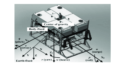
As a practical application of the studied problem framework, we apply our algorithms to the problem of motion coordination of multiple Remotely Operated Vehicles (ROVs). The motion coordination expects the formation of ROVs to rendezvous at a location which is optimal for the formation [16, 14]. The dynamic behavior of ROVs can be described in two coordinate frames, the body-fixed frame and the earth-fix frame as shown in Fig. 2. The dynamics equation of each ROV can be expressed as [44]:
| (46) | ||||
where is the position and orientation described in the earth-fixed frame ( and ), is the linear and angular velocity in the body-fixed frame, and is positive definite, satisfying , is the rigid-body inertia matrix, is the added inertia matrix; is the rigid-body Coriolis and centripetal matrix, is the hydrodynamic Coriolis and centripetal matrix in cluding added mass, is hydrodynamic damping and lift matrix, is a vector of gravitational forces and moment, is the control force and torque vector, is the bounded disturbance vector. Note that system (46) can be transformed into the form of system (1) by choosing the state variables .
As reported in [44], in the positioning and trajectory tracking control of ROV, the variables needed to be controlled are and . Under some cases, for the purpose of improving the dynamic stability and decreasing the influences of and on other variables, a simple P-controller can be used to control and . Therefore the order of the MIMO backstepping robust controller can be reduced from 6 degrees of freedom (DOF) to 4 DOF.
To simplify the controller design, the transformation matrix can also be approximately obtained by assuming that , then the corresponding matrix parameters of reduced system are , , and
According to [44], the velocity dynamics can be expressed as linear-parametric form
where is unknown system parameter vector, is the virtual control and is a known reduced regressor matrix function whose specific form can be found in [44] and is omitted here for saving space.
TABLE I. Simulation Model Parameters of ROV
Par Value Par Value 2500kg -2140kg 1250kgm2 -1636kg 24525N -3000kg 24525N -1524kgm2 -3610kg/s -952 kg/m -4660kg/s -1361kg/m -11772kg/s -3561kg/m -7848kgm2/(srad) -773kgm2/(srad)
Consider a ROV formation which consists of 4 same ROVs. The parameters of the ROV are shown in Table I. The communication topology is given by a -regular graph and the edge weight . The problem of multi-agent coordination consisting in finding a distributed control strategy that is able to drive each ROV from its initial position to rendezvous at the target position which minimizes the square sum of distances from these initial positions. The coordination control objective can be formulated as the following problem:
| (47) |
where represents the initial state of the th ROV.
Next, we apply the proposed secure DOC control strategy to complete the motion coordination task. Consider the cyber attacks (also including the sensor faults or some extraneous factors such as ocean currents) occurring in the complex underwater environment. When the cyber core detects the existence of the cyber attacks, it will drive the attacked ROV to the secure state . In the simulation, the initial state conditions of these four ROVs are set as , , and . Assume that the 4th ROV suffers the cyber attack at s, and . For simplifying calculation, only the ARR rather than is used in the proposed ADI approach.
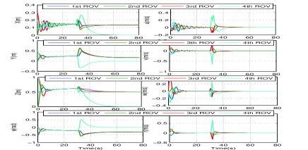
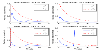
The simulation results are shown in Figs. 3-5. Fig. 3 describes the state responses of and of these four ROVs, . It can be seen that these four ROVs are arriving at the consensus at the optimal solution of (47) before the attack occurs. The ADI mechanism based on the ARR formulated by and is shown in Fig. 4, which implies that for , the ARR generated by is still satisfied even after the cyber attack occurs, while is immediately violated (about at s), thus indicating the cyber attack occurs in the 4th ROV. After detecting the cyber attack, the module will send the control command to the 4th ROV based on the secure decision-making (45). Then the ROV stops sending the transmission data , and converges to the secure position , while the remaining three ROVs achieve the consensus at the optimal solution of
| (48) |
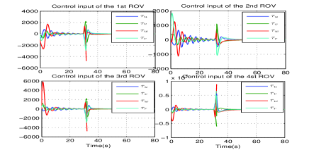
These have been illustrated in Fig. 3. The control inputs of the overall procedure are plotted in Fig. 5.
To further visualize the motion coordination of the ROV formation, also for comparison, the routes of the formulation of ROVs under the following three cases are presented in Figs. 7-9, respectively, where the Simulink in MATLAB running time is set as [0s,80s]:
Case 1: Apply the basic/secure version of DOC under attack-free environment;
Case 2: Apply the basic version of DOC (without the ADI mechanism and secure countermeasure, i.e., set and all the time) under adversarial environment;
Case 3: Apply the secure version of DOC under adversarial environment.
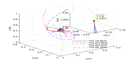
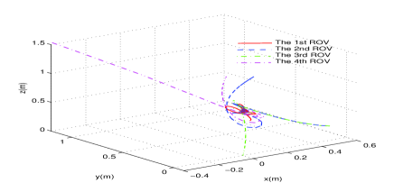
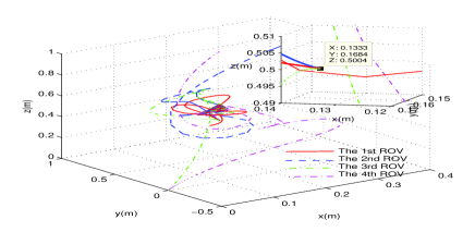
In Fig. 6, clearly all the ROVs rendezvous at the target position (the optimal solution of problem (47)) under the healthy condition. Fig. 7 shows that under the case when the 4th ROV is attacked, all the ROVs follow the wrong control commands and move along with wrong (insecure) routes due to the attack propagation through the exchange of information between neighboring subsystems (The Simulink reports “ERROR” at s and terminates). However, by applying the secure DOC scheme, the ROVs 1, 2 and 3 rendezvous at the target position (the optimal solution of problem (48)), and the 4th ROV reach the preset secure position , which has been illustrated in Fig. 8.
8 Conclusions
This paper presented a secure DOC method for a class of uncertain nonlinear CPSs. First, a basic DOC under the healthy conditions was proposed. By interacting and coordinating between cyber dynamics and physical dynamics, the consensus and optimality were guaranteed. In the presence of multiple cyber attacks, we proposed a distributed ADI approach to identify the locally occurring attacks from multiple propagating attacks. It is shown that any attack signal cannot bypass the designed ADI approach to destroy the convergence of the DOC algorithm. Finally, a secure countermeasure strategy against cyber attacks was described, which guarantees that all healthy physical subsystems complete the DOC objective, while the attacked physical subsystems converge to a given secure state.
Appendix I
Proof of Theorem 1. First, we give the convergence analysis on the cyber dynamics (15) and physical dynamics (1) based on the Lyapunov method, respectively.
Cyber dynamics: Let be a solution of (4). By Lemma 1-(ii), there exists such that holds, and is the saddle of . Consider the Lyapunov function of the cyber dynamics
Note that under the healthy conditions. Then (15) becomes
| (49) | ||||
The time derivative of along with (49) is
| (50) |
where the equalities: follows from and the linearity of in its second argument; follows from the convexity of in the first argument; follows from the fact that is the saddle point of . Note that the mismatching terms and will be compensated by the following physical dynamics.
Physical system: The convergence analysis is discussed based on backstepping procedure. Rewrite (1) into a compact form
| (51) |
where and .
The error dynamics can be expressed as
| (52) |
which can be spitted into inner-loop and outer-loop subsystems:
| (53) |
and
| (54) |
where for .
Next, we provide the Lyapunov analysis of the physical dynamics by considering
where , , .
The derivative of can be computed as
where and represent the inner-loop and outer-loop Lyapunov derivatives, respectively.
Consider the inner-loop error dynamics (53) with controls (16)-(18) and adaptive laws (22)-(24). Following the traditional backstepping procedure [36], along with (53), we can obtain
| (55) |
Now we consider the outer-loop error dynamics (54) with controls (19)-(21).
Step 1. In view of (54) and (15), we have
| (56) |
To stabilize (56), consider the Lyapunov derivative . Then using the virtual control (19), we have
| (57) |
Step . Note that the arguments of the function involve and . From (54) and (15), we have
| (58) |
By using the triangular inequality, one has
Also, on the compact set , there exists a positive constant such that for all . Based on these facts, the Lyapunov derivative along with (58) can be expressed as
| (59) |
Combining (57) and (59), the outer-loop Lyapunov derivative satisfies
| (60) |
Finally, construct the Lyapunov function for the overall CPS. Taking (50), (55) and (60) into account, its time derivative satisfies
| (61) |
where the fact is used.
Choose . Then . Thus, is an invariant set. It implies that , , , , , and are bounded. Then is bounded. Along with the backstepping procedure, , and are also bounded. Noting and . According to Barbalat’s Lemma, and . Finally, following the proof of [[8]. Theorem 4.1], one obtains that . Thus, we can conclude that .
Appendix II
Proof of Lemma 2. To analyze the stability of (30), we first construct an auxiliary system
| (62) |
By directly computing (62), we obtain that
Also, along with (62), the time derivative of the Lyapunov function is
| (63) |
On the other hand, the time derivative of along with (30) can be expressed as
| (64) |
where the inequality follows from the convexity of .
Using the comparison principle [46], under the same initial condition , (63) and (64) imply , or equivalently, .
Directly solving (31) and applying the triangular inequality, can be bounded by (33).
Appendix III
Proof of Lemma 3. Under the healthy conditions, integrating both sides of Eq. (61) yields
which implies that
Given Assumption 3 and definition of , we have
In addition, from Theorem 1 we know is bounded, which yields for any . To prove the result we suppose, for contradiction, there exists such that . According to the form of and the prescribed performance technique [39], converges to . Then as , a contradiction, which in turn implies .
References
- [1] P. Antsaklis, “Goals and challenges in cyber-physical systems research editorial of the editor in chief,” IEEE Trans. Automat. Control, vol. 59, no. 12, pp. 3117–3119, Dec. 2014.
- [2] J. Slay and M.Miller, “Lessons learned from the Maroochy Water Breach,” in Critical Infrastructure Protection. New York, NY, USA: Springer, 2007.
- [3] J. P. Farwell and R. Rohozinski, “Stuxnet and the future of cyber war,” Survival, vol. 53, no. 1, pp. 23–40, 2010.
- [4] A. Nedic and A. Ozdaglar, “Distributed subgradient methods for multiagent optimization,” IEEE Trans. Autom. Control, vol. 54, no. 1, pp. 48–61, 2009.
- [5] I. Lobel and A. Ozdaglar, “Distributed subgradient methods for convex optimization over random networks,” IEEE Trans. Autom. Control, vol. 56, no. 6, pp. 1291–1306, June 2011.
- [6] M. Zhu and S. Martlnez, “On distributed convex optimization under inequality and equality constraints,” IEEE Trans. Autom. Control, vol. 57, no. 1, pp. 151–164, 2012.
- [7] B. Johansson, T. Keviczky, M. Johansson, and K. H. Johansson, “Subgradient methods and consensus algorithms for solving convex optimization problems,” in Proc. IEEE Conf. Decision Control, Cancun, Mexico, Dec. 2008, pp. 4185–4190.
- [8] B. Gharesifard and J. Cortes, “Distributed continuous-time convex optimization on weight-balanced digraphs,” IEEE Trans. Autom. Control, vol. 59, no. 3, pp. 781–786, Mar. 2014.
- [9] C. Y. Kim, D. Z. Song, Y. L. Xu, J. G. Yi, and X. Y. Wu. “Cooperative search of multiple unknown transient radio sources using multiple paired mobile robots,” IEEE Trans. Robotics, vol. 30, no. 5, pp. 1161–1173, 2014.
- [10] E. Dall’Anese, H. Zhu, and G. B. Giannakis, “Distributed optimal power flow for smart microgrids,” IEEE Trans. Smart Grid, vol. 4, no. 3, pp. 1464–1475, 2013.
- [11] S. Bose, S. H. Low, T. Teeraratkul, and B. Hassibi, “Equivalent relaxations of optimal power flow,” IEEE Trans. Autom. Control, vol. 60, no. 3, pp. 729–742, 2015.
- [12] Y. Zhang, Z. Deng, and Y. Hong, “Distributed optimal coordination for multiple heterogeneous Euler-Lagrangian systems,” Automatica, vol. 79, pp. 207–213, 2017.
- [13] P. Lin, W. Ren, Y. Song, and J.A. Farrell, “Distributed optimization with the consideration of adaptivity and finite-time convergence,” in Proc. Conf. Amer. Control, 2014, pp. 3177–3182.
- [14] Y. Xie and Z. Lin,“Global optimal consensus for higher-order multi-agent systems with bounded controls,” Automatica, vol. 99, pp. 301–307, 2019.
- [15] Y. Zhang and Y. Hong, “Distributed optimization design for high-order multi-agent systems,” in Proc. Conf. Chin. Control, 2015, pp. 7251–7256.
- [16] Y. Zhao, Y. Liu, G. Wen, and G. Chen, “Distributed optimization for linear multiagent systems: edge- and node-based adaptive designs,” IEEE Trans. Autom. Control, vol. 62, no. 7, pp. 3602-3609, 2017.
- [17] Z. Li, Z. Wu, Z. Li, and Z. Ding, “Distributed optimal coordination for heterogeneous linear multi-agent systems with event-triggered mechanisms,” IEEE Trans. Autom. Control, 10.1109/TAC.2019.2937500.
- [18] T. Yang, X. Yi, J. Wu, Y. Yuan, D. Wu, Z. Meng, Y. Hong, H. Wang, Z. Lin, K. H. Johansson, “A survey of distributed optimization,” Ann. Rev. Control, vol. 47, pp. 278–305, 2019.
- [19] O. Yaggan, D. Qian, J. Zhang, and D. Cochran, “Optimal allocation of interconnecting links in cyber-physical systems: interdependence, cascading failures, and robustness,” IEEE Trans. Paral. Distr. Syst., vol. 23, no. 9, pp. 1708–1721, 2015.
- [20] L. Su and N. Vaidya, “Byzantine multi-agent optimization,” arXiv:1506.04681, 2015.
- [21] S. Sundaram and B. Gharesifard, “Distributed optimization under adversarial nodes,” IEEE Trans. Autom. Control, vol. 64, no. 3, pp. 1063–1076, 2019.
- [22] C. Zhao, J. He, and Q.-G. Wang, “Resilient distributed optimization algorithm against adversarial attacks,” IEEE Trans. Autom. Control, 10.1109/TAC.2019.2954363.
- [23] W. Fu, J. Qin, Y. Shi, W. Zheng, and Y. Kang, “Resilient consensus of discrete-time complex cyber-physical networks under deception attacks,” IEEE Trans. Ind. Inf., 10.1109/TII.2019.2933596.
- [24] Q. Zhang and X. Zhang, “Distributed sensor fault diagnosis in a class of interconnected nonlinear uncertain systems,” in Proc. 8th IFAC SAFEPROCESS, Mexico City, Mexico, 2012, pp. 1101–1106.
- [25] V. Reppa, M. M. Polycarpou, and C. G. Panayiotou, “Decentralized isolation of multiple sensor faults in large-scale interconnected nonlinear systems,” IEEE Trans. Autom. Control, vol. 60, no. 6, pp. 1582–1596, Mar. 2015.
- [26] V. Reppa, M. M. Polycarpou, and C. G. Panayiotou, “Distributed sensor fault diagnosis for a network of interconnected cyber-physical systems,” IEEE Trans. Control Netw. Syst., vol. 2, no. 1, pp. 11–23, Mar. 2015.
- [27] L. Zhang and G.-H. Yang, “Observer-based fuzzy adaptive sensor fault compensation for uncertain nonlinear strict-feedback systems,” IEEE Trans. Fuzzy Syst., vol. 26, no. 4, pp. 2301–2310, 2018.
- [28] F. Pasqualetti, F. Dorfler, and F. Bullo, “Attack detection and identification in cyber-physical systems,” IEEE Trans. Autom. Control, vol. 58, no. 11, pp. 2715–2729, 2013
- [29] L. An and G.-H. Yang, “Distributed secure state estimation for cyber-physical systems under sensor attacks,” Automatica, vol. 107, pp. 526–538, 2019.
- [30] J. Zhang, R. Blum, X. Lu, and D. Conus, “Asymptotically optimum distributed estimation in the presence of attacks,” IEEE Trans. Signal Process., vol. 63, no. 5, pp. 1086–1101, Mar. 2015.
- [31] M. Zhu and S. Mart nez, “Attack-resilient distributed formation control via online adaptation,” in Proc. IEEE Conf. Dec. Control Eur. Control (CDC-ECC), Orlando, USA,, 2011, pp. 6624–6629.
- [32] L. An and G.-H. Yang, “Data-driven coordinated attack policy design based on adaptive -gain optimal theory,” IEEE Trans. Autom. Control, vol. 63, no. 6, pp. 1760–1767, 2018.
- [33] Y. Liu, M.K. Reiter, and P. Ning, “False data injection attacks against state estimation in electric power grids,” in Proc. the 16th ACM conf. Computer communications security, 2009, pp. 21–32.
- [34] Y. Chen, S. Kar, and J.M.F. Moura, “Optimal attack strategies subject to detection constraints against cyber-physical systems,”IEEE Trans. Control Netw. Syst., vol. 5, no. 3, pp. 1157–1168, 2019.
- [35] T.-Y. Zhang and D. Ye, “False data injection attacks with complete stealthiness in cyber-physical systems: A self-generated approach,” Automatica, vol. 120, Oct. 2020, Art. no. 109117.
- [36] M. Krstic, P. V. Kokotovic, I. Kanellakopoulos, Nonlinear and Adaptive Control Design. New York: Wiley, 1995.
- [37] H. Ouyang, Y. Lin, “Adaptive fault-tolerant control for actuator failures: A switching strategy,” Automatica, vol. 81, pp. 87–95, 2017.
- [38] X. D. Tang, G. Tao, and S. M. Joshi, “Adaptive actuator failure compensation for parametric strict feedback systems and an aircraft application,” Automatica, vol. 39, pp. 1975–1982, 2003.
- [39] W. Wang and C. Wen, “Adaptive actuator failure compensation control of uncertain nonlinear systems with guaranteed transient performance,” Automatica, vol. 46, pp. 2082–2091, 2010.
- [40] W. Wang, C. Wen, J. Huang, “Distributed adaptive asymptotically consensus tracking control of nonlinear multi-agent systems with unknown parameters and uncertain disturbances,” Automatica, vol. 77, pp. 133–142, 2017.
- [41] W. Liu and J. Huang, “Adaptive leader-following consensus for a class of higher-order nonlinear multi-agent systems with directed switching networks,” Automatica, vol. 79, pp. 84–92, 2017.
- [42] M. Massoumnia, G. Verghese, and A. Willsky, “Failure detection and identification,” IEEE Trans. Autom. Control, vol. 34, no. 3, pp. 316–321, 1989.
- [43] H. Fawzi, P. Tabuada, and S. Diggavi, “Secure estimation and control for cyber-physical systems under adversarial attacks,” IEEE Trans. Automat. Control, vol. 59, no. 6, pp. 1454–1467, Jun. 2014.
- [44] K. Zhu, L. Gu, “A MIMO nonlinear robust controller for work-class ROVs positioning and trajectory tracking control,” in Proc. Annu. Conf. Control Decision, Hangzhou, China, 2011, pp. 2565–2570.
- [45] A. Eldosouky, A. Ferdowsi, and W. Saad, “Drones in distress: a game-theoretic countermeasure for protecting UAVs against GPS spoofing,” IEEE Int. Things Journal, vol. 7, no. 4, 2840–2854, 2020.
- [46] H. Khalil, Nonlinear Systems, third ed., Prentice Hall, Hoboken, New Jersey, 2002.