Research
Phil. Trans. R. Soc. A
xxxxx, xxxxx, xxxx
M. Drissi
Second-order optimisation strategies for neural network quantum states
2 Department of Physics, University of Surrey, Guildford GU2 7XH, United Kingdom
3 Departament de Física Quàntica i Astrofísica, Universitat de Barcelona (UB), c. Martí i Franquès 1, E08028 Barcelona, Spain
4 Institut de Ciències del Cosmos (ICCUB), Universitat de Barcelona (UB), Barcelona, Spain
Abstract
The Variational Monte Carlo method has recently seen important advances through the use of neural network quantum states. While more and more sophisticated ansätze have been designed to tackle a wide variety of quantum many-body problems, modest progress has been made on the associated optimisation algorithms. In this work, we revisit the Kronecker Factored Approximate Curvature, an optimiser that has been used extensively in a variety of simulations. We suggest improvements on the scaling and the direction of this optimiser, and find that they substantially increase its performance at a negligible additional cost. We also reformulate the Variational Monte Carlo approach in a game theory framework, to propose a novel optimiser based on decision geometry. We find that, on a practical test case for continuous systems, this new optimiser consistently outperforms any of the KFAC improvements in terms of stability, accuracy and speed of convergence. Beyond Variational Monte Carlo, the versatility of this approach suggests that decision geometry could provide a solid foundation for accelerating a broad class of machine learning algorithms.
keywords:
neural network quantum states, variational Monte Carlo, game theory, decision geometry, optimisation1 Introduction
Neural network quantum states (NQS) have been recently employed to represent the ground state wave functions of several quantum many-body systems [1, 2, 3, 4, 5, 6, 7, 8, 9, 10, 11]. These state-of-the-art machine learning (ML) tools allow for numerically efficient solutions of the Schrödinger equation, while keeping the relevant information of the wave function in a finite, relatively small number of parameters. The primary focus of NQS has been to leverage advancements in ML to represent the widest class of many-body wave functions. The first NQS was developed in Ref. [1], where a Restricted Boltzmann Machine was used to model spin systems. More recently, the field of quantum chemistry has seen a surge of ansätze representing the wave function of many-electron systems [2, 3, 4, 5, 6]. Message-passing architectures have also been proposed to tackle strongly correlated fermionic systems [8, 11, 10]. A key ingredient of many of these NQS is the use of permutation-equivariant layers. These provide an efficient representation of the required antisymmetry of fermionic many-body wave functions.
To tackle the quantum many-body problem, NQS are usually formulated in the framework of variational Monte Carlo (VMC) [12, 13]. Like any variational approach, VMC calculates the ground-state of a many-body system by minimising the expectation value of the energy of an associated Hamiltonian over a class of trial wave functions. Provided the class is large enough, this approach should yield a good approximation of the ground state, even in the case of strongly interacting particles. Monte Carlo techniques are employed to estimate the many-body, and generally high-dimensional, integral for the ground-state energy. In practice, with NQS, one reformulates the physics energy minimisation process in terms of a ML reinforcement learning problem. The loss function is the total energy of the system, and the wave function is learned by minimising it.
In nuclear physics, specifically, NQS have shown promising results. Starting from a simple solution to the deuteron [14], the field has quickly evolved towards fully-fledged nuclear structure calculations [15, 16, 17]. Further advances in architectures have opened the window to applications in periodic systems [18] like neutron matter [19], and in models based on the occupation number formalism [9]. The NQS reformulation may be able to surpass previous efforts in VMC simulations of nuclear systems [20, 21]. While simulations have not yet reached the level of sophistication of other ab initio methods [22, 23, 24], NQS have the potential to become a new and competitive first-principles technique.
Clearly, the optimisation algorithm in this minimisation process plays a critical role to achieve results efficiently. In the most challenging cases, typically involving many particles, the wall-time per epoch may increase substantially. With these cases in mind, one may want to design optimisation strategies that reduce the total number of epochs. Typically, optimisation strategies are based on gradient descent methods, which exploit the first-order derivatives of the loss function with respect to the variational parameters. In a ML setting, derivatives are efficiently estimated using automatic differentiation (AD) techniques [25]. A possible approach to accelerate the optimisation consists in approximating second-order derivatives of the loss function to incorporate information on the local curvature in the update of the parameters. This typically leads to a trade-off, where the total number of epochs to converge accurately is reduced at the price of increasing the wall-time per epoch.
The Adam [26] and the Kronecker Factored Approximate Curvature (KFAC) [27] optimisers have been extensively used in the NQS community. While Adam provides a stable and robust optimisation strategy, its convergence to accurate results is generally fairly slow. As an example, Refs. [3, 7] indicate that Adam requires between to epochs to reach an accuracy of in the correlation energy. In contrast, KFAC has been shown to work remarkably well [27, 28, 29] and has become a key factor in VMC calculations for the most challenging cases [3, 5, 6, 30]. However, the KFAC optimiser was originally designed for supervised learning problems [27] and has mostly been tested with standard feed-forward neural networks (NN). Despite several extensions, for example to include convolutional layers [28], the justification of its applicability to VMC with NQS remains unclear. As a matter of fact, to bypass problems encountered with KFAC in VMC, several groups have come up with a series of ad hoc adjustments to rectify a posteriori the update on the parameters obtained from KFAC [3]. These adjustments go against the philosophy originally advocated in Ref. [27], which suggested that the learning rate and momentum should be automatically adjusted based on the exact Fisher matrix, and where the damping was dynamically adjusted using a Levenberg-Marquardt rule.
In this work, we revisit the original KFAC optimiser and review its formulation within a VMC-NQS framework. We aim to tackle its shortcomings at the very basis, in order to build a new versatile optimiser that may accelerate VMC calculations for a wide variety of many-body problems. We introduce in Sec. 2 the quantum many-body problem that we use as a testbed: strongly-interacting polarised fermions in a one-dimensional harmonic trap. The NQS ansatz used in VMC and the general KFAC algorithm are also briefly discussed. Then, in Sec. 3, we single out several important issues that we encountered with the original implementation of KFAC. We show how these relate to fundamental aspects of VMC and NQS, namely the use of the energy as a loss function and the use of permutation equivariant layers. From this analysis, we build a new improved KFAC-like optimiser that addresses directly these issues and shows a dramatic improvement in terms of stability and accuracy. Finally, in Sec. 4, we revisit the underlying information geometry [31, 32] on which KFAC is built [27]. We reformulate the VMC problem in a game theory setting, which motivates an alternative decision geometry [33, 34, 35]. A novel optimiser based on this decision geometry is then introduced, which outperforms any of the previously tested optimisers.
2 Quantum many-body model
2.1 System and Hamiltonian
In the following, we provide a general discussion on optimisation strategies for quantum many-body systems. For concreteness and pedagogical purposes, several aspects of the discussion are illustrated with a simple many-body system [7]. The toy model we consider is a system of fermions of mass , trapped in a one-dimensional harmonic well [7]. For simplicity, we assume the system to be fully polarised and thus neglect spin effects. We employ Harmonic Oscillator (HO) units and choose a Gaussian-shaped two-body interaction with range and strength , inspired by nuclear-physics applications [7]. The Hamiltonian of the system thus reads
| (1) |
Throughout this work, we use this system as a toy model to benchmark the performance of different energy optimisation schemes. Specifically, we change the number of particles from to and the interaction strength, , from to . We keep a fixed interaction range, , which allows for an exploration of the non-perturbative regime [7].
This system has the advantage to be simple while displaying an interesting phenomenology. Its simplicity allows us to explore many different optimisation scenarios while, its phenomenological diversity supports the fact that our conclusions can not be too specific to the many-body problem we consider. In particular, when varying between and , the many-body system undergoes a transition from a strongly attractive regime, where spinless fermions behave like a non-interacting bosonic system [36, 37, 38], to a strongly repulsive regime, akin to that of a crystal [39, 40].
As an illustrative example, we show in Fig. 1 the one-body density profile, , as a function of the spatial position for the system. The different panels correspond to different interaction strengths. We show our NQS prediction with a solid line, but provide also two additional benchmarks. Dashed lines correspond to a configuration interaction (CI) result. This employs a full direct diagonalisation of the Hamiltonian within a given configuration space [41]. The associated Hartree-Fock (HF) results are shown with dash-dotted lines.
The central panel (c) shows the non-interacting case, . It displays an overall Gaussian-like profile with a series of superimposed peaks, which are characteristic of fermion systems. Panels (a) and (b), to the left of the center, show the attractive regime with and , respectively. In this region, the wiggles disappear and the density profile acquires a dumbbell shape. This relatively featureless density profile is reminiscent of a bosonic system [7]. In this regime, the CI results disagree with the NQS prediction because of the truncation of the model space, which is performed for practical numerical reasons. Here, and in the following, we will not show CI results for for this reason. In contrast, the HF results agree relatively well with the NQS prediction in the attractive regime.
Panels (d) and (e) correspond to the repulsive regime for values of the interaction strength and . They suggest a very different behaviour of the density profile in the repulsive regime. The system does not change substantially in average size, but the fermionic oscillations on top of the smooth behaviour become much more pronounced. This is a sign of localisation, or crystallisation, in the system. We note that here the HF density profile differs substantially from the NQS result, although the energy predictions (not shown here) are relatively close to the NQS predictions. For more details on the physics of this model, we refer to our previous work in Ref. [7].

2.2 The Variational Monte Carlo method
To compute the ground state of the Hamiltonian in Eq. (1) we follow a VMC approach [12] and aim at solving the many-body problem using the Rayleigh-Ritz variational principle,
| (2) |
where denotes the exact -body ground-state energy of . In VMC, the wave function is not in general the exact ground state, but rather a trial wave function that depends on a series of parameters. Using the Rayleigh-Ritz variational principle, the original eigenvalue problem can thus be recast as an optimisation problem in the subspace of trial wave functions.
In practice, three major challenges need to be faced to solve this optimisation problem. First of all, the Hilbert space of -body states in the optimisation search is in principle infinite-dimensional. This difficulty is usually tackled by introducing the much smaller set of trial states over which the energy is minimised. In doing so, a bias is introduced on the solution, which is usually estimated by varying the size of the set of trial states. A second difficulty comes from the necessity to evaluate the expectation value of the energy over many different trial states. Each estimate consists of an integral of at least dimension , where denotes the number of space dimensions. To mitigate the cost of evaluating these high-dimensional integrals, one resorts to Monte Carlo estimates, which necessarily introduce a statistical noise on the energy. This can in principle be controlled by using a large enough number of samples in the Monte Carlo estimate. Finally, the third challenge is to find the solution of a global non-linear optimisation problem. Here, the established strategy consists in breaking the problem into a sequence of simpler, local-quadratic optimisation sub-problems, which are solved iteratively. Such iterative optimisers have the advantage of versatility and can be used for many different optimisation problems. However, they often require adjustments to converge in a reasonable time [42].
The third challenge is the main focus of this work, and we will address it in the Section 3. Before diving into it, we provide some details on our NQS strategy which will be useful to frame the global discussion on the optimisation strategy.
2.3 Neural Quantum States and Monte Carlo sampling
Our NQS ansatz is a fully antisymmetric NN, inspired by the implementation of FermiNet [3]. The inputs to our network are the positions of fermions in the system, , and the output is the many-body wave function in the log domain. The state depends on a series of network weights and biases, succinctly summarised by a variable of dimension [7]. The network is composed of core components: equivariant layers, generalised Slater matrices (GSMs), Gaussian log-envelope functions, and a summed signed-log determinant function [43]. The equivariant layers have the particularity of sharing a common set of weights and biases among the input positions. This weight sharing is critical in order to enforce total antisymmetry of the wave function and, as discussed later, will impact the rationale justifying KFAC. For all calculations presented in this work, the number of equivariant layers is set to ; their width, , is ; and we only use one GSM. We stress that the orbitals making a GSM are functions depending on the positions of all the particles, thus departing from a standard Slater matrix. These so-called backflow correlations are key in obtaining a faithful representation of the exact state [7]. In total, our wave function ansatz depends on about parameters, which have to be optimised to solve the many-body problem.
The expectation value of the energy, in Eq. (2), is typically formulated as a statistical average over local energies,
| (3) |
where we define as an -dimensional random variable (or walker) distributed according to the Born probability of the many-body wave function, . For numerical stability, the kinetic energy is computed in the log domain. For a general local interaction, the local energy in a continuous model reads
| (4) |
For our specific model, the interaction terms are
| (5) |
To sample the statistical averages over the Born probability , we use walkers propagated following a Metropolis-Hastings algorithm (MH) [44, 45] with on-the-fly adaptation of the proposal distribution width [30]. In order to neglect any biases due to autocorrelation in our comparison of multiple optimisers, we perform MH iterations per epoch, to ensure the thermalisation of the Markov chain. The optimisation process requires not only the evaluation of the energy expectation value, , but also the gradients with respect to all the parameters of the network . These are evaluated as a statistical average according to
| (6) |
Finally, to provide a reasonable starting point to the energy minimisation algorithms, we drive the NQS through a pre-training phase. This is a supervised learning problem, where we demand that the network reproduce the many-body wave function of the non-interacting system. The goal is to obtain an initial state that is physical and somewhat similar, in terms of spatial extent, to the result after the interaction is switched on. This also helps speed up the simulation in the more demanding cases [43, 7]. Throughout this work, the parameters of the network are randomly initialised before going through pre-training epochs using the Adam optimiser. The final pretrained NQS is the starting point for all the optimisation algorithms that we consider. For a given particular system (number of particles and interaction strength ), we always start from the same exact NQS and set of samples. This guarantees that any differences that arise in the optimisation process are due to the optimisers themselves. We refer the reader to the Supplementary Material and to Refs. [43, 7] for more details on the Monte Carlo sampling and the pre-training used in our calculations.
3 KFAC within a Variational Monte Carlo framework
3.1 General optimisation strategy
Solving a global, non-linear optimisation problem is a difficult task. In this work, we consider optimisers that follow the same underlying strategy, sometimes referred to as sequential quadratic programming [42]. In our case, the general problem takes the form,
| (7a) | ||||
| (7b) | ||||
This problem is divided into a sequence of simpler sub-problems which are solved iteratively. The sub-problem consists of (a) an initial guess on the set of parameters, ; (b) a quadratic model, , approximating the loss function locally; and (c) a trust region, , specifying where the local model is expected to be a good approximation to the loss function [42]. Formally, solving the sub-problem consists in computing a new energy estimate, , at the updated parameters, , namely
| (8a) | ||||
| (8b) | ||||
Here, represents the update in the parameters and the quadratic model takes the form
| (9) |
where is a matrix; , a vector; and , a scalar. In practice, the constrained quadratic optimisation sub-problem is replaced by an equivalent unconstrained regularised sub-problem,
| (10) |
where is a damping parameter, characterising the size of the equivalent trust region and is a symmetric positive semi-definite matrix describing the shape of the trust region. This procedure is often referred to as Tikhonov regularisation [46, 42]. Importantly, not only are the energy and the parameters, , updated at each iteration, but also the local quadratic model and its trust region (or regularisation), .
As an instructive example, the standard gradient descent method can be formulated in this framework. In this case, one solves iteratively the locally constrained sub-problems associated to the model
| (11) |
with trust region
| (12) |
where denotes the standard Euclidean norm. In this case, the update on the parameter reads explicitly
| (13) |
When solving this sequence of local constrained sub-problems, one is effectively performing a gradient descent with a learning rate .
3.2 Natural Gradient Descent
Equations (11)-(12) indicate that the standard gradient descent algorithm relies on setting an isotropic constraint on the size of the update parameter, , based on the Euclidean norm. In a general setting, the Euclidean norm has no reason to be an optimal choice. Different gradient descent algorithms have been designed in an attempt to outperform the standard version presented in the previous subsection. The natural gradient descent (NGD) algorithm, which has been advocated to be optimal for a class of optimisation problems, is of particular interest [47, 48]. This algorithm is the starting point of the KFAC optimiser [27].
The NGD was originally defined in a supervised learning setting, where the goal is to learn an empirically sampled distribution by minimising a loss function. One particular loss function, chosen here for pedagogical reasons, is the cross-entropy, namely
| (14) |
Here, is a probability distribution, depending on several parameters , that is adjusted to minimise the cross-entropy loss. In this case, the manifold of the probability distributions possesses a natural geometry commonly referred to as information geometry [31, 32]. The information geometry is defined by the Kullback-Leibler (KL) divergence between two probability distributions
| (15) |
Although the KL divergence does not satisfy all the axioms of a distance, it defines locally a metric obtained by Taylor-expanding it at second-order, namely
| (16) |
where is the Fisher information matrix (FIM). The expansion is performed around the "diagonal" point, . From the expansion, one obtains an explicit expression for the FIM,
| (17) |
where and are individual components of the global parameter vector, . In this context, the NGD consists simply in performing a gradient descent with a trust region defined by the norm associated to the FIM. For example, where denotes the maximum size of an update on . As mentioned earlier, it is more practical to work with an equivalent unconstrained regularised problem. In the case of NGD for VMC, the regularised local model is
| (18) |
where the damping is a function of the size of . Equivalently, the update minimising can be expressed as
| (19) |
where is a learning rate related to the size of .
In practice, NGD has been shown to be efficient for specific kinds of supervised learning problems [47, 48]. Additionally, stochastic reconfiguration, a quantum generalization of NGD, has been observed to perform well in the context of VMC [49, 50, 9]. The exact reasons for the success of the NGD are still under study [29]. Apart from empirical tests, two critical properties of the FIM have been raised for explaining its performance: (i) the FIM is symmetric definite positive and (ii) it provides an approximation to the Hessian of the loss function in the case of supervised learning [29]. Point (i) is important to avoid instabilities in the directions associated to negative eigenvalues of the quadratic term, so that updates in the parameters remain bounded. Point (ii) leads to a re-interpretation of the NGD as a second-order optimisation scheme, where the Hessian of the loss function is approximated by the FIM. This motivates the minimisation of a model
| (20) |
This interpretation leads to the update
| (21) |
which is equivalent to fixing the learning rate to unity, , in Eq. (19).
3.3 KFAC algorithm
A practical implementation of the NGD algorithm requires computing the update in Eq. (21). In the case of NN models, the number of parameters, , is large (). Computing exactly the update at every epoch can be computationally prohibitive. The goal of the KFAC algorithm is to compute an approximation to the update with a time complexity of while keeping the number of epochs to convergence roughly constant. We note that, for the specific case of NQS, there are alternative proposals to implement this update calculations employing fast Jacobian-vector product algorithms [51, 52, 53].
Consider a feed-forward NN of arbitrary depth. For a given layer , we denote the weight matrix and, for simplicity, we assume it to be of size and without bias. The input row-vector and the output row-vector are related according to where the activation function is applied element-wise111We focus on this activation function because it is the one of choice in our NQS model [7], but any other choice would not change our conclusions. . In this work, we follow the convention used in the PyTorch framework where inputs and outputs of a layer are row vectors.
In the KFAC algorithm originally described in Ref. [27], the FIM is approximated in two ways. First, the matrix elements between parameters of different layers are neglected. The approximated FIM, , is block-diagonal and reads
| (22) |
where is the parameter associated to the matrix element of the layer weight matrix. Second, each layer-dependent block is approximated by a Kronecker product. Using the chain rule, the FIM derivatives can be rewritten as
| (23) |
Introducing the so-called forward activations, , and the backward sensitivities, , as the row vectors
| (24a) | ||||
| (24b) | ||||
we obtain
| (25) |
where and denote respectively the standard vectorisation (stacking columns of a matrix) and Kronecker product operations. Using Eq. (25), the block of the FIM can be rewritten in vectorised form as
| (26) |
Finally, the Kronecker-factored approximation on the block of the FIM, , is obtained by exchanging the order of the Kronecker product and the statistical average, i.e.
| (27) |
The resulting block-diagonal KFAC FIM will be denoted as from now on.
Assuming a unit learning rate, the update in the parameters when using the KFAC approximation thus reads
| (28) |
We employ a capital to differentiate it from previous parameter updates. The main advantage of the KFAC approximation is that, instead of having to invert a matrix of dimension , one can invert separately the Kronecker factors in Eq. (27), which are much smaller matrices of dimension . The main drawback is that the KFAC approximation is very crude and can only catch the very coarse structure of the exact FIM [27]. For completeness, let us also mention that the two Kronecker factors are averaged over successive epochs, with a maximum exponentially decay value set to [27].
To compensate for the poor quality of the update , a second step was designed in the original KFAC algorithm [27]. The idea is that, whenever provides a good direction, we would like to take a big step. In contrast, when the direction is poor, we would like to take a small step, to avoid increasing the loss function. In the original KFAC algorithm, this is achieved by computing an optimal rescaling factor such that the quadratic model , which uses the exact FIM, is minimised. In addition, a momentum in the previous update is usually included. A natural way to include both improvements consists in minimising over the two parameters and . Explicitly, the optimal coefficients and are obtained from the linear system
| (29) |
where we momentarily drop the superindex KFAC in all the and updates for simplicity. Using the exact FIM is crucial to help correct cases where the KFAC approximation is too crude. This correction remains relatively cheap, since Eq. (29) only requires computing a couple of matrix-vector calculations.
Last but not least, the original derivation of KFAC describes a particular Tikhonov regularisation in order to stabilise the overall algorithm [27]. Such a regularisation is of critical importance, since it limits how large the update in the parameters can be. If the trust region is too small, the benefits of using a second-order optimiser will be null. If the trust region is too large, instabilities will kick in and ruin any chances of reaching convergence.
The KFAC FIM is used to estimate the direction of the update, while the exact FIM is used to evaluate an optimal rescaling of the direction. Consequently, two distinct trust regions are considered, which reflect the different level of trust one has in the direction, , and the rescaling factor, . Those are implemented by introducing two damping factors, and , which regularise and , respectively. More explicitly, the regularised matrices are obtained from the substitutions
| (30a) | ||||
| (30b) | ||||
where is a factor that is automatically adjusted to minimise the cross-term obtained when expanding the Kronecker product [27]. In practice, the damping factors are dynamically adapted every epochs.
While we try to be as close to the original KFAC algorithm as possible, our numerical implementation for the NQS toy model slightly differ in the dynamically adjustment of the damping factors. The damping factor is adapted following a Levenberg-Marquardt rule [54], namely
| (31) |
The reduction ratio,
| (32) |
measures the discrepancy between the actual variation of the loss (numerator) and the anticipated one from the quadratic model (denominator). Unlike in the original KFAC implementation, however, we also account for fluctuation on the energy estimation by introducing a tolerance on increasing the energy, i.e. if , we default to the case where the damping is reduced. In all our calculations is set to of . The damping is adapted with a greedy algorithm by testing which damping among leads to the best update. For all the calculations performed in this work, we set , , and the initial damping values are set to and . For clarity, we provide a schematic overview of the KFAC algorithm in Fig. 2. For more details, we refer the reader to Ref. [27].

3.4 Improving the scaling estimation
Since its inception, the KFAC optimiser has been tested on several deep autoencoder optimisation problems with standard datasets (MNIST, CURVES and FACES), which are commonly used to benchmark NN optimisation methods [55, 56]. The focus of these models is on supervised learning, with a standard feed-forward NN. Beyond such standard cases, the original KFAC optimiser may need to be adapted. For instance, if convolution layers are a part of the NN architecture, Refs. [28, 57] suggest modifications to the KFAC approximation to the FIM. In the case of VMC with NQS, several attempts have been put forward to exploit the benefits of KFAC [3, 30, 58]. To bypass instabilities encountered when applying the standard KFAC optimiser, several ad hoc adjustments have been implemented to rectify the update on the parameters [3]. In particular, Ref. [3] describes the use of a scheduled learning rate, a constant damping, a norm constraint and the discarding of any momentum in the parameter updates. Apart from the lack of theoretical motivation for such adjustments, it is consistently reported within the literature that heuristics and fine-tuning are required to obtain good performance [3, 30, 58].
In this section, we advocate for a different approach, which avoids any such heuristic adjustment of hyperparameters, while remaining close to the original philosophy of Ref. [27]. We start by providing an overview of the performance associated to our NQS KFAC implementation for the toy model described in Sec. 2, before suggesting improvements to the formulation of the algorithm. We show the evolution of the energy as a function of the epoch in the panels of Fig. 3. From top to bottom, the different rows correspond to increasing number of particles, from in the top to in the bottom row. From left to right, the results scan the interaction strength in a range . Dashed lines provide an indication of the expected results for the HF approximation and for the CI case. The optimisation process in all cases is stopped after epochs. Very few minimisations reach this final number and most lead to numerically unstable results much earlier than that. As in previous NQS implementations[3, 30, 58], we confirm that the performance of the KFAC optimiser is indeed fluctuating. In many cases, the energy decreases steadily within the first to epochs, only to become extremely erratic after that point. None of the KFAC runs manage to converge to the benchmark values, regardless of the number of particles and of the strength of the interaction. We take this as a confirmation that the KFAC algorithm, in its original formulation, is unreliable for VMC with NQS.

One option to compensate the strong oscillations is to try and improve the rescaling phase of the optimiser. The main argument put forward in favour of using in the rescaling phase is that the FIM can be interpreted as an approximation to the Hessian of the loss function [27, 29]. However, as emphasized in Refs. [27, 29], the validity of this argument relies critically on the assumption that one is trying to solve a supervised learning problem. In this case, the loss function quantifies how far the probability distribution , modelled by the NN, is from the target distribution, . An example of such loss function is the cross-entropy, given in Eq. (14). In VMC, however, one is solving a reinforcement learning problem, which is fundamentally different. In this case, the loss function is the energy which characterises the quality of the NQS independently of the knowledge of the target wave function. Consequently, the underlying rationale justifying the use of the FIM as an approximate Hessian is lost.
In order to restore the validity of KFAC in VMC calculations, we replace the exact FIM used in the rescaling phase by a quasi-Hessian matrix, , whose role is to provide a better quadratic model than , namely
| (33) |
Throughout this work, we will refer to the resulting optimisation algorithm as quasi-Newton KFAC (QN-KFAC), and we employ the superscript QN in the corresponding quantities. For supervised learning problems, the performance of NGD has been connected to the similarity between the FIM and the Generalised-Gauss-Newton matrix [29]. Specifically, this matrix can be obtained by neglecting the Hessian of the output of the NN in the calculation of the Hessian of the loss function [29]. To improve the rescaling phase of the algorithm, we follow a similar path and define the quasi-Hessian as the matrix obtained from the Hessian of the energy , after neglecting the Hessian of . More specifically, the Hessian of the energy reads
| (34) |
Neglecting the first line, the induced quasi-Hessian reads
| (35) |
A key advantage of using a quasi-Hessian with this structure is that matrix-vector operations can be performed as fast as for the FIM. However, a critical drawback is that the is not in general positive semi-definite, which can lead to instabilities if the damping is not large enough. In addition, the formula given in Eq. (35) requires to compute third-order derivatives of the wave function. These arise from the second-order derivatives with respect to the input in the kinetic energy term of the local energy, and the derivatives with respect to the parameters. These derivatives should be handled with care in order to avoid numerical instabilities [3]. A schematic overview of the QN-KFAC algorithm is provided in Fig. 2.
We now proceed to compare the VMC energy evolution employing QN-KFAC and KFAC. We stress that we perform systematic calculations with all hyperparameters of the two optimisers kept fixed to the aforementioned values (see also the Supplementary Material). This minimises the differences in the optimisation scheme and provides a general overview in different physical conditions. We observe that QN-KFAC (green lines) leads to a dramatic increase in overall stability. We find that for a small number of particles, , QN-KFAC almost always manages to converge to reasonable values. For larger particle numbers, the convergence pattern is more erratic. In some cases, we notice strong oscillations. In others, we observe jumps in energy predictions. The best-behaved convergence patterns are found for and . While this improvement is encouraging, we also notice that, even in the best cases, the late stage convergence can be slow. For instance, if we focus on the second column, corresponding to , we observe that, after a quick convergence during the first epochs, the QN-KFAC optimiser seems to struggle to converge fully before reaching our stopping criterion of epochs. Comparing QN-KFAC with CI in the case (top panel), it is clear that QN-KFAC converged to the exact result. However, for particles and the same interaction strength, in the absence of exact CI benchmarks, it is not clear whether or not the QN-KFAC finished converging.
The QN-KFAC optimiser provides a first improvement over KFAC in our NQS toy model simulations. This was achieved by modifying the quadratic model used in the rescaling phase of the KFAC algorithm. In order to tackle the remaining issues observed when testing QN-KFAC, like the presence of strong oscillations in some cases and the slow convergence pattern in the late stage of the optimisation process, we now proceed to improve on the direction estimation phase of the optimiser.
3.5 Improving the direction estimation
The original KFAC algorithm was developed for supervised learning problems with standard feed-forward NNs. In the case of a reinforcement learning problem like VMC, the theoretical motivation for using the FIM is lost. This prompted the changes discussed in the previous subsection. In this subsection, we further argue that using an NQS architecture additionally breaks the original rationale motivating the Kronecker factorisation, which lies at the heart of the KFAC algorithm [27].
As mentioned in section 3.3, the direction of the update in the parameters is obtained based on two approximations of the complete FIM: (i) the FIM is assumed to be block-diagonal in the layers and (ii) each block is further approximated by exchanging the Kronecker product and the statistical average, thus replacing Eq. (26) by Eq. (27). The latter approximation is discussed at length in the original derivation of KFAC in Ref. [27]. The validity of Eq. (26), however, is unclear. The chain rule used to derive it relies on the specific NN type and architecture. In the case of a standard feed-forward NN, considered in Ref. [27], Eq. (26) does obviously hold. Equation (26) however breaks down in the case of convolution layers and the original KFAC algorithm was adapted accordingly in Ref. [28].
In the case of NQS for fermionic systems, permutation-equivariant layers also break Eq. (26). Specifically, let us consider the permutation-equivariant layer with a shared weight matrix with input and output , related through the activation function Using the chain rule, the derivatives in the FIM for a fermionic NN now read
| (36) |
In this case, the forward activities and backward sensitivities are not row vectors, but rather matrices
| (37a) | ||||
| (37b) | ||||
With this, we recover formally the same result as Eq. (25),
| (38) |
However, because the forward activities and backward sensitivities are now matrices, we no longer find a Kronecker product structure for the partial derivatives, i.e. Instead, the block of the FIM in vectorised form reads
| (39) |
where is the identity matrix. In this result, we have used the general formula [59], which holds for any matrices , and with compatible matrix products. Comparing Eq. (26) to Eq. (39), one sees that the weight-sharing introduces an intermediate factor, , which prevents us from recasting the FIM as the average of a Kronecker product.
Interestingly, this analysis suggests that the KFAC rationale remains valid for the case. We expect that it will become less and less valid as the number of particles, , increases. This seems to support our empirical observation that QN-KFAC performs better for small values of . The results obtained with QN-KFAC in Fig. 3 look indeed more stable, and converge faster, for and than for .
In order to compensate for the incompatibility of the original Kronecker factorisation motivation when employing NQS, we introduce an additional step in QN-KFAC. Our goal is to improve on the direction of the update starting from the one obtained from KFAC. To do so, we use an iterative solver for linear equations. We employ MINRES [60], an algorithm that solves linear systems, for sparse, symmetric matrices, , and output vectors, . The underlying idea of MINRES consists in combining a Lanczos algorithm with an LQ factorisation in order to minimise the squared residual In our case, we use MINRES to find an approximate solution to the system
| (40) |
using as an initial guess. We recall that is the block-diagonal approximation of the FIM as defined in Eq. (26). For simplicity, we choose to reuse to regularise the directional update improvement, instead of . Since we use the block-diagonal FIM without the KFAC in Eq. (40) we consider it to be reasonable to choose the same trust region used for the rescaling (which uses the exact FIM). Following Ref. [61], we also use the preconditioner with and to accelerate the convergence of the linear solver. In addition, MINRES is stopped as soon as we achieve a relative residual smaller than or when the number of iteration reaches a maximum number, . We dub the resulting optimiser QN-MR-KFAC. We note that when , QN-MR-KFAC reduces to QN-KFAC. For clarity, we provide a schematic overview of the QN-MR-KFAC algorithm in Fig. 2.

We now test the impact of using a refined directional update, , instead of the bare KFAC estimate, . We focus first on cases where QN-KFAC converges reasonably well without violent oscillations. We show the energy as a function of the epoch number for with (top panel) and (bottom panel) particles in Fig. 4. Specifically, we illustrate the impact of MINRES by exploring a different set of iterations, .
The results clearly indicate that improving the direction of the parameter update (or increasing ) has two key effects. First, the oscillations in the energy estimate during the minimisation process are substantially reduced. Even for (top panel), where the oscillations were relatively small, increasing leads to substantially reduced oscillations in the energy predictions. For particles (bottom panel), QN-KFAC, which corresponds to the line, has relatively large oscillations in energy, of order in HO units. When increases to , the oscillations are reduced by about a factor of . A further increase up to shows minor oscillations, to less than about in HO units. Second, the convergence in the late stages of the optimisation is considerably faster. For , QN-KFAC only converges to the CI result at around the epoch. When the MINRES solver performs more than iterations per epoch, the optimisation process reaches the CI value in iterations. In the -particle case, the improvement is more dramatic. QN-KFAC plateaus, but does not converge, at the epoch. Increasing , a more transparent convergence pattern appears and, for , about epochs are enough to reach the minimum. We stress that the characteristically slow approach to the minimum was a major drawback of the QN-KFAC proposal.
Overall, we observe that improving the quality of the direction of substantially impact the performances. Comparing the and cases, we see that the number of MINRES iterations necessary to reach optimal convergence is larger as increases. This supports our previous theoretical analysis expecting KFAC to be less and less well motivated as increases. In practice, we find that setting is sufficient for any case where a stable convergence is reached.

A more systematic analysis of the importance of the improvement in the direction of the updates is provided in Fig. 5. Here, we show the same results as in Fig. 3, but comparing QN-KFAC to QN-MR-KFAC with . The results confirm that QN-MR-KFAC greatly improves on both the oscillations of the energy values and the late phase of convergence. In the vast majority of cases, QN-MR-KFAC performs better than QN-KFAC in terms of accuracy and speed of convergence. Concerning the stability of the optimisation process, the improvements are more marginal. The attractive and non-interacting cases (columns to the left of, and including, the center) only show some erratic peaks in energy in a few, selected cases. In contrast, the repulsive cases are still prone to important oscillations as soon as .
Finally, we notice that in several cases (for example when , and , ) QN-MR-KFAC shows instabilities even after having converged. We interpret this behaviour in terms of the dynamically adjusted damping. Once convergence is reached, the trust region keeps increasing. One may eventually hit a remote spurious point in the local quadratic model which has a value that is lower than the true ground-state energy and jump there. The associated numerical instability takes a few epochs to self-adjust. As stated before, this is one of the drawbacks of using a quasi-Hessian, , which is not positive semi-definite. These pathological cases may in principle be cured by introducing a minimum value on the damping, . More generally, most of the fluctuations encountered so far can be tackled by being more restrictive on the trust regions. However, in doing so, we also restrict the size of the updates and slow down the overall convergence of the optimiser. We also introduce the risk of an artificial convergence, in the sense that the energy may converge only because the trust region has shrunk to a very narrow point. We leave further analysis of trust regions and their dynamical adjustments for future work.
4 Decisional gradient descent
4.1 Failure of information geometry
Despite the multiple improvements to the original KFAC algorithm which we designed to take into account the particularities of VMC and NQS, our finest optimiser, QN-MR-KFAC, is still subject to violent fluctuations in the energy. As discussed in Sec. 3.5, this could be tackled by further refining the trust regions. Doing so, however, may limit the original promise of performance or require fine-tuning of the hyperparameters, as in past attempts to adapt KFAC to VMC with NQS [3, 30]. These attempts, including ours, rely on the use of the FIM, , to estimate the direction of the updates . The use of the FIM was originally motivated by its connection to the Hessian of the loss function in a supervised learning setting. We have already argued that standard VMC-NQS does not fall in the category of supervised learning problems, and hence using the FIM (or its corresponding approximations) is no longer justified. The substantial improvement observed in Fig. 3, where the quasi-Hessian is used in the rescaling phase of the optimiser instead of the exact FIM , further supports this idea. We hypothesise that, the failure of KFAC are not only due to the approximations it makes to NGD, but also more fundamentally to the failure of NGD itself to provide a good optimiser for VMC.
To test this hypothesis, we perform calculations with an optimiser that is identical to QN-MR-KFAC with , except that the exact FIM, , as opposed to the quasi-Hessian, , is used in the rescaling phase. This is closer in spirit to Hessian-free optimisers [61]. In addition, to avoid any contamination from KFAC, we replace the initial guess in the MINRES solver by the previous update, rescaled by a prefactor , i.e. the starting point of the MINRES solver is now instead of . This follows the default recommendation of Ref. [61] for Hessian-free optimisers. All other hyperparameters are fixed to the same value used in our previous QN-MR-KFAC calculations. Although we do not calculate exactly the natural gradient update, given in Eq. (21), we deem this to be sufficiently close to the NGD approach. In consequence, we will refer to this optimiser as NGD. A schematic overview of our implementation of NGD is provided in Fig. 2.

We present the results of this NGD optimiser in Fig. 6. The panels are organised in the same fashion as Fig. 3. In all the cases considered, NGD fails to converge smoothly to a final value. We find strong oscillations, akin to those observed for KFAC in Fig. 3. In some cases, particularly in the attractive regime (columns to the left of the center), the optimiser seems to get stuck around the HF solution. Even then, violent oscillations arise in the energy minimisation process. The generic failure of the NGD optimiser across different numbers of particles and interaction strengths further supports our hypothesis that NGD is fundamentally unfit for VMC. As discussed in Sec. 3.2, NGD can be seen as a simple gradient descent where the definition of trust regions are based on information geometry, i.e., on the KL divergence (15). We interpret the failure of NGD as a consequence of the unsuitability of information geometry for VMC.
This raises the question: which geometry should one use for VMC? Ideally, we would like to use a geometry leading to (i) a local metric that is positive semi-definite, for stability purposes; and (ii) a metric informed by the loss function that we are trying to minimise, here the energy . While both conditions are satisfied when considering information geometry for supervised learning problems, condition (ii) is violated in the case of VMC simulations. In order to restore condition (ii), we now introduce the concept of decision geometry.
4.2 Decision geometry
Our starting point consists in reformulating VMC in a game-theory framework. In this paradigm, the standard information geometry is generalised by the concept of decision geometry [62, 63, 34, 32].
Similarly to how the KL divergence, Eq. (15), is related to the cross-entropy loss, Eq. (14), one can define a divergence function associated to any loss function of the type
| (41) |
so long as is a so-called proper scoring rule [35]. A scoring rule is any integrable function that takes as inputs a probability distribution, , and a sample, , and returns a real valued quantity. From any scoring rule, one defines the associated expected score for any two probability distributions and by
| (42) |
A scoring rule is said to be proper if and only if, for any two probability distributions and ,
| (43) |
In this framework, several typical quantities of information theory can be generalised. For example, the generalised entropy and the generalised cross-entropy are simply and , respectively. Their associated divergence function, , is defined by
| (44) |
The new geometry, associated to , is referred as a decision geometry [63, 34] because of its relation with statistical decision problems [64]. Similarly to the KL divergence, defines a metric locally. This is obtained by Taylor-expanding at second-order, namely
| (45) |
where is the decision metric associated to . Let us emphasize that, by construction, is symmetric positive semi-definite.
This symmetric and positive definite decision metric provides a natural starting point for optimisation schemes that are not tied to the FIM. In this context, we define a novel optimiser, the decisional gradient descent (DGD) which consists simply in performing a gradient descent with trust regions defined by the norm associated to the decision metric, Here, denotes the maximum size on the update . Just like for NGD, it is more practical to work with an equivalent unconstrained regularised problem. This leads to the definition of an update
| (46) |
where is again a learning rate that can be related to the size of .
If we choose the scoring rule , the decision geometry framework is such that one recovers exactly the standard cross-entropy, Eq. (14), and the KL divergence, Eq. (15). In other words, DGD reduces to NGD. To go beyond NGD, we move away from the standard logarithmic scoring rule and choose instead an alternative one based on the local energy, namely
| (47) |
We refer to this scoring rule as the VMC scoring rule. The local energy in our toy model is explicitly given in Eq. (4). One can show that, for such local energy, the inequality
| (48) |
holds. In other words, is a proper scoring rule. Following the analogy with information geometry, the total energy , computed as the expectation value of the local energy, is analogous to a generalised entropy
| (49) |
with associated divergence
| (50) |
For our toy model, employing continuous variables in a one-dimensional setting and a local interaction term, Eq.(4), this difference reduces to the expectation value
| (51) |
This divergence arises entirely from the kinetic term of the Hamiltonian, which is the reason why derivatives appear. We note that this divergence can be written in terms of first-, rather than second-order derivatives, because we assume regularity at the boundaries. For our neural network it can be analytically proven that the boundary terms appearing in the derivation of the divergence are zero, and therefore Eq. (51) holds exactly. However, this need not be the case for arbitrary NN architectures or distributions.
As can be seen from Eq. (50), the decision geometry obtained from the VMC scoring rule defined in Eq. (47) provides a connection between the geometry and the loss function we aim to minimise, . Indeed, the divergence we obtain can be seen as an approximation of the difference of energy , where we would have neglected re-weighting the samples. The metric, , obtained from Taylor-expanding the divergence thus fulfills the two main theoretical requirements we discussed in Sec. 4.1, namely (i) the metric is symmetric positive definite and (ii) the metric is informed by the loss function we aim to minimise. The metric reads explicitly
| (52) |
and we will use it later on in simulations. A peculiarity of this equation is the appearance of mixed derivatives with respect to both parameters and inputs of the probability distribution. We will provide more details on the DGD optimiser in a forthcoming publication [65].
Interestingly, using the very natural scoring rule of Eq. (47) for VMC leads to a geometry that is equivalent to the one introduced by Hyvärinen from very different initial considerations [66, 67, 32]. In Ref. [66], the main concern was to bypass the difficulty of sampling according to a non-normalised probability distribution. The so-called Hyvärinen score has the following form
| (53) |
and it is essentially the kinetic part of the local energy, Eq. (4). Our VMC score is related to the Hyvärinen score through the formula As a result, the associated divergence function and metric are proportional to each other, i.e. their decision geometry are identical up to a scaling factor. In the language of game theory, the Hyvärinen and VMC scoring rules are said to be equivalent [34, 35].
4.3 Application to VMC
We now proceed to test a DGD-based optimisation strategy on VMC calculations with NQS. In this case, one uses the VMC scoring rule, Eq. (47), which defines the metric . Moreover, the loss function is the energy of the system, so the update in the parameters immediately reads
| (54) |
In order to provide a fair comparison with NGD and the associated approximated optimisers (KFAC, QN-KFAC or QN-MR-KFAC), we have set the learning rate . This common choice is critical to ensure that any success of DGD is well motivated and that DGD can be interpreted as a second-order optimiser. In this case, one solves the sequence of quadratic sub-problems
| (55) |
As a first implementation of DGD, we use the very same code employed in our NGD optimiser. The difference is that we replace the FIM in the NGD, by the decision metric, . We provide a schematic overview of the implementation of DGD in Fig. 2 and remind the reader that more information on hyperparameters can be found in the Supplementary Material.
Results for the NGD and DGD optimisers are shown hand in hand in Fig. 6. Clearly, the stability of the optimisation process is dramatically improved when employing DGD. A well-defined initial minimisation occurs for the first epochs in all cases. Importantly, the energy minimum is usually reached within this first epochs. No strong fluctuations are observed in the energy either close or away from the minimum. Out of the cases presented in Fig. 6, only three extreme cases (i.e. about of the minimisations) fail to converge. Explicitly, these cases correspond to particles with and with and with . In the first two cases, the lack of convergence is seen in terms of an energy drift at large numbers of epochs, which happens after a short plateau close to the physical minimum. In the latter case, a numerical instability precludes any minimisation past epochs. Let us stress that all the simulations shown in Fig. 6 employed the exact same set of hyperparameters (see Supplementary Material). In this context, it does not seem unreasonable to expect that further refinements of the DGD optimisation algorithm may lead to a systematic convergence to the ground-state energy.

We provide further insight on the performance of the DGD optimiser in Fig. 7, where we compare it to our best NGD-based optimiser, QN-MR-KFAC. Overall, we observe that the DGD optimiser generally performs as well as, if not better than, QN-MR-KFAC in terms of accuracy and speed of convergence. In the attractive regime, corresponding to the panels left and including the central column, we find that the two optimisers perform almost equally well. DGD, however, improves on the stability of the minimisation, avoiding the jumps that QN-MR-KFAC shows during the minimisation process. Similar conclusions hold for the repulsive regime (panels right to the central column), although some of the cases with are challenging for both optimisers.
Compared to NGD, we interpret the overall improvement of DGD in terms of the direct link that is established between the local model and the loss function. Compared to QN-MR-KFAC, the fact that we keep a positive semi-definite metric, unlike the quasi-Hessian of Eq. (35), is also an advantage that avoids the instabilities discussed in Sec. 3.5.
As an additional example that showcases the optimisation power of DGD, we now proceed to compare DGD results with Adam [26]. We have relied on Adam in the NQS applications of Ref. [7], where we employ the default hyperparameters and a learning rate of . In that case, we train the network to minimise the energy for epochs. This relatively long training process is required to guarantee the convergence of the energy, which is particularly slow in the last part of the training, when approaching the energy minimum.
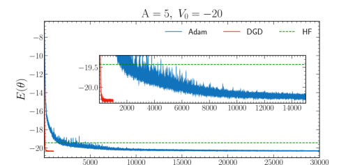
In Fig. 8, we display illustrative results for and for Adam and DGD. The results show that the number of epochs required to reach a similar level of accuracy in the energy minimum is dramatically reduced when using DGD. Such speed-up is even more pronounced when we focus on the correlation stage i.e. when comparing the number of epochs to converge, starting from the epoch where the HF energy has been reached. Interestingly, the fluctuations on the energy value between epochs are also substantially reduced. DGD achieves oscillations that are well within in HO units within a few hundred epochs. In contrast, Adam only reaches a similar level of accuracy well past epochs.
We note that we have performed more extensive comparisons between DGD and Adam and we show these in the Supplemental Material. These extensive comparisons indicate that, while the number of epochs that Adam requires to converge increases with , the performance of DGD stays relatively constant. This should be helpful for tackling larger system in future NQS simulations. Overall, compared to Adam, DGD shows a strong adaptability to the optimisation problem and a particularly high performance in the late stage of convergence. Those two empirical features are typical of second-order optimisers [29].
Finally, let us also comment on the wall-time associated to the different methods. DGD brings in a substantial acceleration in terms of wall-time, thanks to the reduction in the number of epochs. A timing profile of our NQS implementation [68] indicates that the dominant time factor is the Markov Chain Monte Carlo (MCMC) propagation. Our MCMC is particularly demanding, because we have run simulations with a large number of MH steps in order to avoid autocorrelation issues. It is likely that the wall-time per epoch can be reduced further by setting a more reasonable number of MH iterations per epoch. This would affect the peformance of both Adam and DGD. Further quantification of the numerical complexity of the DGD optimiser are left for future work.
5 Conclusion and outlook
NQS are a promising new tool in quantum many-body physics. In nuclear physics, these methods hold the promise to become a competitive ab initio approach, tackling nuclei from first principles. In particular, given their VMC underpinning, these methods may reach relatively large particle numbers with a commensurate computational cost. The extension of NQS techniques to heavier systems requires technical developments for the energy optimisation process. Here, we have focused on improving existing state-of-the-art optimisation schemes for NQS.
We have compared several optimisation schemes on a one-to-one basis. We employ the setting and toy model of Ref. [7] as a test bed, which has a rich phenomenology in spite of its simplicity. We hope that the conclusions we draw can be extrapolated to other systems. We mainly focus on the KFAC algorithm, that has been extensively employed in past NQS simulations [3]. Our numerical analysis indicates that KFAC cannot be employed safely in a general VMC-NQS setting. We find a series of large oscillations in the minimisation process for a wide variety of physical properties. KFAC was originally designed for tackling supervised learning problems with feed-forward NNs. Instead, VMC falls into the category of reinforcement learning problems and NQS architectures are rarely simple feed-forward networks. New and original approaches are necessary in order to recover the performance of second-order optimisers within a general VMC-NQS setting.
In an effort to remedy the situation, we first propose two variants of KFAC that try to bridge the gap towards VMC-NQS. First, to account for the fact that VMC is not a supervised learning problem, we replace the exact FIM used in the rescaling phase by an approximation of the Hessian of the energy, which can be computed easily but is not positive-definite. The resulting approach, dubbed QN-KFAC, is more stable than the original KFAC implementation, but its convergence is still erratic in half the cases. Second, to adapt KFAC to a general NQS, we propose an improvement in the direction estimation of the parameter updates using the MINRES iterative linear solver. This allows us to mitigate the breaking of the Kronecker factorization due to the permutation-equivariant structure of our NQS. The resulting optimisation scheme, QN-MR-KFAC, is much more stable and accurate than any of the previous optimisers. In spite of the improvements, this optimiser still shows instabilities and spikes in energy, even close to the minimum.
Our third and last attempt to improve the optimisation of NQS is a radical departure from KFAC. Instead of employing information geometry to inform the learning process of our model, we take a decisional approach based on game theory developments. This allows us to design an optimisation scheme that is tailored to our VMC calculations. The associated decision geometry defines an alternative positive semi-definite metric which restores the link between geometry and loss function. This so-called DGD method has a similar computational cost to others, but provides a much faster, and much more stable, minimisation pattern. A relatively simple implementation of DGD shows already a fast and stable convergence in more than of the cases. Because our toy model is relatively generic but incorporates a wide phenomenology, we expect similar improvements in other quantum many-body systems. In particular, we hope that our optimisation strategies will be useful in developing NQS further for nuclear physics applications.
The overall stability of DGD indicates that it has superior capabilities when it comes to VMC as compared to KFAC or any of the resulting approaches we derived. Many improvements on this first implementation of DGD can already be anticipated. To mention just a few, one could improve the stability and speed of convergence by implementing a better damping scheme, following Ref. [61]. The overall wall-time could also be reduced by replacing the iterative linear solver, MINRES, with another one minimising directly the quadratic sub-problem in Eq. (55). Recently, some groups have also proposed alternative approximations to KFAC that aim at reducing the cost of solving linear systems at each epoch [52, 51, 69]. Adapting those techniques to DGD could lead to important reductions of the wall-time per epoch.
We note also that other attempts at designing better metrics than the FIM have recently appeared [70]. In this context, decision geometry provides a framework of choice due its high degree of flexibility. In particular, it is intriguing that the potential energy, a crucial characterisation of the optimisation problem, cancels out in the generation of the divergence in Eq. (51). Building new divergence functions incorporating information on the potential energy could be an interesting avenue to further refine the geometry to the particular optimisation problem. We are currently working on exploiting this flexibility to study spin lattice systems [65]. Finally, beyond considerations on VMC and NQS, the versatility of decision geometry suggests that it could be a promising avenue to design fast and robust optimisation strategies for a broad class of machine learning problems.
Conflict of Interest Statement
The authors declare that the research was conducted in the absence of any commercial or financial relationships that could be construed as a potential conflict of interest.
This work is supported by STFC, through Grants Nos ST/L005743/1 and ST/P005314/1; by grant PID2020-118758GB-I00 funded by MCIN/AEI/10.13039/501100011033; by the “Ramón y Cajal" grant RYC2018-026072 funded by MCIN/AEI /10.13039/501100011033 and FSE “El FSE invierte en tu futuro”; by the “Consolidación Investigadora" Grant CNS2022-135529 funded by MCIN/AEI/ 10.13039/501100011033 and by the “European Union NextGenerationEU/PRTR”; by the “Unit of Excellence María de Maeztu 2020-2023" award to the Institute of Cosmos Sciences, Grant CEX2019-000918-M funded by MCIN/AEI/10.13039/501100011033. TRIUMF receives federal funding via a contribution agreement with the National Research Council of Canada. This work has been financially supported by the Ministry of Economic Affairs and Digital Transformation of the Spanish Government through the QUANTUM ENIA project call - Quantum Spain project, and by the European Union through the Recovery, Transformation and Resilience Plan - NextGenerationEU within the framework of the Digital Spain 2026 Agenda. The authors gratefully acknowledge the computer resources at Artemisa, funded by the European Union ERDF and Comunitat Valenciana as well as the technical support provided by the Instituto de Fisica Corpuscular, IFIC (CSIC-UV).
Supplementary material
We provide a Supplementary Material file.
Data, code and materials
The source code used for this study can be found in the GitHub repository https://github.com/jwtkeeble/second-order-optimization-NQS.
References
- [1] Carleo G, Troyer M. 2017 Solving the quantum many-body problem with artificial neural networks. Science 355, 602–606. (10.1126/science.aag2302)
- [2] Hermann J, Spencer J, Choo K, Mezzacapo A, Foulkes WMC, Pfau D, Carleo G, Noé F. 2023 Ab initio quantum chemistry with neural-network wavefunctions. Nat. Rev. Chem. 7, 692–709. (10.1038/s41570-023-00516-8)
- [3] Pfau D, Spencer JS, Matthews AG, Foulkes WMC. 2020 Ab initio solution of the many-electron Schrödinger equation with deep neural networks. Phys. Rev. Res. 2, 033429. (10.1103/PhysRevResearch.2.033429)
- [4] Hermann J, Schätzle Z, Noé F. 2020 Deep-neural-network solution of the electronic Schrödinger equation. Nat. Chem. 12, 891–897. (10.1038/s41557-020-0544-y)
- [5] Spencer JS, Pfau D, Botev A, Foulkes WMC. 2020 Better, faster fermionic neural networks. arXiv preprint arXiv:2011.07125. (10.48550/arXiv.2011.07125)
- [6] von Glehn I, Spencer JS, Pfau D. 2022 A Self-Attention Ansatz for Ab-initio Quantum Chemistry. arXiv preprint arXiv:2211.13672. (10.48550/arXiv.2211.13672)
- [7] Keeble JWT, Drissi M, Rojo-Francàs A, Juliá-Díaz B, Rios A. 2023 Machine learning one-dimensional spinless trapped fermionic systems with neural-network quantum states. Phys. Rev. A 108, 063320. (10.1103/PhysRevA.108.063320)
- [8] Pescia G, Nys J, Kim J, Lovato A, Carleo G. 2023 Message-Passing Neural Quantum States for the Homogeneous Electron Gas. arXiv preprint arXiv:2305.07240. (10.48550/arXiv.2305.07240)
- [9] Rigo M, Hall B, Hjorth-Jensen M, Lovato A, Pederiva F. 2023 Solving the nuclear pairing model with neural network quantum states. Phys. Rev. E 107, 025310. (10.1103/PhysRevE.107.025310)
- [10] Kim J, Pescia G, Fore B, Nys J, Carleo G, Gandolfi S, Hjorth-Jensen M, Lovato A. 2023 Neural-network quantum states for ultra-cold Fermi gases. arXiv preprint arXiv:2305.08831. (10.48550/arXiv.2305.08831)
- [11] Lou WT, Sutterud H, Cassella G, Foulkes WMC, Knolle J, Pfau D, Spencer JS. 2023 Neural Wave Functions for Superfluids. arXiv preprint arXiv:2305.06989. (10.48550/arXiv.2305.06989)
- [12] Becca F, Sorella S. 2017 Quantum Monte Carlo Approaches for Correlated Systems. Cambridge University Press. (10.1017/9781316417041)
- [13] Martin RM, Reining L, Ceperley DM. 2016 Interacting Electrons: Theory and Computational Approaches. Cambridge University Press. (10.1017/CBO9781139050807.007)
- [14] Keeble J, Rios A. 2020 Machine learning the deuteron. Phys. Lett. B 809, 135743. (10.1016/j.physletb.2020.135743)
- [15] Adams C, Carleo G, Lovato A, Rocco N. 2021 Variational Monte Carlo Calculations of Nuclei with an Artificial Neural-Network Correlator Ansatz. Phys. Rev. Lett. 127, 022502. (10.1103/PhysRevLett.127.022502)
- [16] Gnech A, Adams C, Brawand N, Carleo G, Lovato A, Rocco N. 2022 Nuclei with Up to A=6 Nucleons with Artificial Neural Network Wave Functions. Few-Body Syst. 63, 7. (10.1007/s00601-021-01706-0)
- [17] Gnech A, Fore B, Lovato A. 2023 Distilling the essential elements of nuclear binding via neural-network quantum states. arXiv preprint arXiv:2308.16266. (10.48550/arXiv.2308.16266)
- [18] Pescia G, Han J, Lovato A, Lu J, Carleo G. 2022 Neural-network quantum states for periodic systems in continuous space. Phys. Rev. Res. 4, 023138. (10.1103/PhysRevResearch.4.023138)
- [19] Fore B, Kim JM, Carleo G, Hjorth-Jensen M, Lovato A, Piarulli M. 2023 Dilute neutron star matter from neural-network quantum states. Phys. Rev. Res. 5, 033062. (10.1103/PhysRevResearch.5.033062)
- [20] Carlson J, Gandolfi S, Pederiva F, Pieper SC, Schiavilla R, Schmidt KE, Wiringa RB. 2015 Quantum Monte Carlo methods for nuclear physics. Rev. Mod. Phys. 87, 1067–1118. (10.1103/RevModPhys.87.1067)
- [21] Lomnitz-Adler J, Pandharipande VR, Smith RA. 1981 Monte Carlo calculations of triton and 4He nuclei with the Reid potential. Nucl. Phys. A 361, 399–411. (10.1016/0375-9474(81)90642-4)
- [22] Hagen G, Papenbrock T, Hjorth-Jensen M, Dean DJ. 2014 Coupled-cluster computations of atomic nuclei. Rep. Prog. Phys. 77, 096302. (10.1088/0034-4885/77/9/096302)
- [23] Hergert H, Bogner SK, Morris TD, Schwenk A, Tsukiyama K. 2016 The In-Medium Similarity Renormalization Group: A novel ab initio method for nuclei. Phys. Rep. 621, 165–222. (10.1016/j.physrep.2015.12.007)
- [24] Somà V. 2020 Self-Consistent Green’s Function Theory for Atomic Nuclei. Front. Phys. 8. (10.3389/fphy.2020.00340)
- [25] Baydin AG, Pearlmutter BA, Radul AA, Siskind JM. 2018 Automatic differentiation in machine learning: a survey. J. Mach. Learn. Res. 18, 1–43. (10.48550/arXiv.1502.05767)
- [26] Kingma D, Ba J. 2015 Adam: A Method for Stochastic Optimization. In International Conference on Learning Representations (ICLR). (10.48550/arXiv.1412.6980)
- [27] Martens J, Grosse R. 2015 Optimizing neural networks with Kronecker-factored approximate curvature. In International conference on machine learning pp. 2408–2417. (10.48550/arXiv.1503.05671)
- [28] Grosse R, Martens J. 2016 A Kronecker-factored approximate Fisher matrix for convolution layers. In NeurIPS pp. 573–582. (10.48550/arXiv.1602.01407)
- [29] Martens J. 2020 New insights and perspectives on the natural gradient method. J. Mach. Learn. Res. 21, 5776–5851. (10.48550/arXiv.1412.1193)
- [30] Wilson M, Gao N, Wudarski F, Rieffel E, Tubman NM. 2021 Simulations of state-of-the-art fermionic neural network wave functions with diffusion Monte Carlo. arXiv preprint arXiv:2103.12570. (10.48550/arXiv.2103.12570)
- [31] Amari Si. 1983 A foundation of information geometry. Electron. Commun. Jpn. (Part I: Commun.) 66, 1–10. (10.1002/ecja.4400660602)
- [32] Amari Si. 2016 Information geometry and its applications vol. 194. Springer. (10.1007/978-4-431-55978-8)
- [33] Dawid AP, Lauritzen SL. 2005 The geometry of decision theory. In Proceedings of the Second International Symposium on Information Geometry and its Applications pp. 22–28. University of Tokyo.
- [34] Dawid AP. 2007 The geometry of proper scoring rules. Ann. Inst. Stat. Math. 59, 77–93. (10.1007/s10463-006-0099-8)
- [35] Gneiting T, Raftery AE. 2007 Strictly proper scoring rules, prediction, and estimation. J. Am. Stat. Assoc. 102, 359–378. (10.1198/016214506000001437)
- [36] Girardeau MD, Olshanii M. 2003 Fermi-Bose mapping and N-particle ground state of spin-polarized fermions in tight atom waveguides. arXiv preprint cond-mat/0309396. (10.48550/arXiv.cond-mat/0309396)
- [37] Granger BE, Blume D. 2004 Tuning the Interactions of Spin-Polarized Fermions Using Quasi-One-Dimensional Confinement. Phys. Rev. Lett. 92, 133202. (10.1103/PhysRevLett.92.133202)
- [38] Valiente M. 2020 Bose-Fermi dualities for arbitrary one-dimensional quantum systems in the universal low-energy regime. Phys. Rev. A 102, 053304. (10.1103/PhysRevA.102.053304)
- [39] Wigner E. 1934 On the interaction of electrons in metals. Phys. Rev. 46, 1002. (10.1103/PhysRev.46.1002)
- [40] Ziani N, Cavaliere F, Becerra K, Sassetti M. 2020 A Short Review of One-Dimensional Wigner Crystallization. Crystals 11. (10.3390/cryst11010020)
- [41] Rojo-Francàs A, Polls A, Juliá-Díaz B. 2020 Static and Dynamic Properties of a Few Spin 1/2 Interacting Fermions Trapped in a Harmonic Potential. Mathematics 8, 1196. (10.3390/math8071196)
- [42] Nocedal J, Wright SJ. 2006 Numerical optimization. Springer New York, NY. (10.1007/978-0-387-40065-5)
- [43] Keeble J. 2022 Neural Network Solutions to the Fermionic Schrödinger Equation. PhD thesis University of Surrey. (10.15126/thesis.900505)
- [44] Metropolis N, Ulam S. 1949 The Monte Carlo method. J. Am. Stat. Assoc. 44, 335–341. (10.1080/01621459.1949.10483310)
- [45] Hastings WK. 1970 Monte Carlo sampling methods using Markov Chains and their applications. Biometrika 57, 97–109. (10.1093/biomet/57.1.97)
- [46] Baumeister J. 1987 Stable Solution of Inverse Problems. Advanced Lectures in Mathematics. Vieweg+Teubner Verlag Wiesbaden. (10.1007/978-3-322-83967-1)
- [47] Amari Si. 1998 Natural Gradient Works Efficiently in Learning . Neural Comput. 10, 251–279. (10.1162/089976698300017746)
- [48] Amari S, Douglas S. 1998 Why natural gradient?. In Proceedings of the 1998 IEEE International Conference on Acoustics, Speech and Signal Processing, ICASSP ’98 (Cat. No.98CH36181) vol. 2 pp. 1213–1216 vol.2. (10.1109/ICASSP.1998.675489)
- [49] Sorella S. 2005 Wave function optimization in the variational Monte Carlo method. Phys. Rev. B 71, 241103. (10.1103/PhysRevB.71.241103)
- [50] Stokes J, Izaac J, Killoran N, Carleo G. 2020 Quantum Natural Gradient. Quantum 4, 269. (10.22331/q-2020-05-25-269)
- [51] Rende R, Viteritti LL, Bardone L, Becca F, Goldt S. 2023 A simple linear algebra identity to optimize large-scale neural network quantum states. arXiv preprint arXiv:2310.05715. (10.48550/arXiv.2310.05715)
- [52] Chen A, Heyl M. 2023 Efficient optimization of deep neural quantum states toward machine precision. arXiv preprint arXiv:2302.01941. (10.48550/arXiv.2302.01941)
- [53] Vicentini F, Hofmann D, Szabó A, Wu D, Roth C, Giuliani C, Pescia G, Nys J, Vargas-Calderón V, Astrakhantsev N, Carleo G. 2022 NetKet 3: Machine Learning Toolbox for Many-Body Quantum Systems. SciPost Phys. Codebases p. 7. (10.21468/SciPostPhysCodeb.7)
- [54] Moré JJ. 2006 The Levenberg-Marquardt algorithm: implementation and theory. In Numerical Analysis: Proceedings of the Biennial Conference Held at Dundee pp. 105–116. Springer. (10.1007/BFb0067700)
- [55] Hinton GE, Salakhutdinov RR. 2006 Reducing the dimensionality of data with neural networks. Science 313, 504–507. (10.1126/science.1127647)
- [56] Martens J. 2010 Deep Learning via Hessian-Free Optimization. In Proceedings of the 27th International Conference on International Conference on Machine Learning ICML’10 p. 735–742. Omnipress. Available at https://www.cs.toronto.edu/ jmartens/docs/Deep_HessianFree.pdf.
- [57] Ba J, Grosse R, Martens J. 2017 Distributed second-order optimization using Kronecker-factored approximations. In International Conference on Learning Representations. Available at https://jimmylba.github.io/papers/nsync.pdf.
- [58] Wilson M, Moroni S, Holzmann M, Gao N, Wudarski F, Vegge T, Bhowmik A. 2022 Wave function ansatz (but periodic) networks and the homogeneous electron gas. arXiv preprint arXiv:2202.04622. (10.48550/arXiv.2202.04622)
- [59] Henderson HV, Searle SR. 1981 The vec-permutation matrix, the vec operator and Kronecker products: A review. Linear Multilinear Algebra 9, 271–288. (10.1080/03081088108817379)
- [60] Paige CC, Saunders MA. 1975 Solution of sparse indefinite systems of linear equations. SIAM J Numer. Anal. 12, 617–629. (10.1137/0712047)
- [61] Martens J, Sutskever I. 2012 Training deep and recurrent networks with hessian-free optimization. In Neural Networks: Tricks of the Trade , pp. 479–535. Springer. (10.1007/978-3-642-35289-8_27)
- [62] Topsøe F. 1979 Information-theoretical optimization techniques. Kybernetika 15, 8–27.
- [63] Grünwald PD, Dawid AP. 2004 Game theory, maximum entropy, minimum discrepancy and robust Bayesian decision theory. Ann. Stat. 32, 1367. (10.1214/009053604000000553)
- [64] Ferguson TS. 1967 Mathematical Statistics: A Decision Theoretic Approach. Academic Press. (10.1016/C2013-0-07705-5)
- [65] Keeble J, Drissi M, Rozalén Sarmiento J, Rios A. 2024 A decisional step in Variational Monte Carlo. In preparation.
- [66] Hyvärinen A. 2005 Estimation of Non-Normalized Statistical Models by Score Matching. J. Mach. Learn. Res. 6, 695–709. Available at http://jmlr.org/papers/v6/hyvarinen05a.html.
- [67] Hyvärinen A. 2007 Some extensions of score matching. Comput. Stat. Data Anal. 51, 2499. (10.1016/j.csda.2006.09.003)
- [68] Azzam A. 2023 Transfer Learning For Many-Body Systems. Master’s Thesis University of Barcelona. Available at http://hdl.handle.net/2445/202717.
- [69] Goldshlager G, Abrahamsen N, Lin L. 2024 A Kaczmarz-inspired approach to accelerate the optimization of neural network wavefunctions. arXiv preprint arXiv:2401.10190. (10.48550/arXiv.2401.10190)
- [70] Sasaki T, Miyahara H. 2024 Quantum natural gradient without monotonicity. arXiv preprint arXiv:2401.13237. (10.48550/arXiv.2401.13237)