Second order hydrodynamics based on effective kinetic theory and electromagnetic signals from QGP
Abstract
We study the thermal dilepton and photon production from relativistic heavy ion collisions in presence of viscosities by employing the recently developed second order dissipative hydrodynamic formulation estimated within a quasiparticle description of thermal QCD (Quantum Chromo-Dynamics) medium. The sensitivity of shear and bulk viscous pressures to the temperature dependence of relaxation time is analyzed within one dimensional boost invariant expansion of quark gluon plasma (QGP). The dissipative corrections to the phase-space distribution functions upto first order in gradients are obtained from the Chapman-Enskog like iterative solution of effective Boltzmann equation in the relaxation time approximation. Thermal dilepton and photon production rates for QGP are calculated by employing this viscous modified distribution function. Yields of these particles are quantified for the longitudinal expansion of QGP with different temperature dependent relaxation times. Our analysis employing this second order hydrodynamic model indicates that the spectra of dileptons and photons gets enhanced by both bulk and shear viscosities and is well behaved. Also, these particle yields are found to be sensitive to relaxation time. Further, we do a comparison of these particle spectra with a standard hydrodynamic formulation.
I Introduction
The experiments at Relativistic Heavy Ion Collider (RHIC) and at Large Hadron Collider (LHC) suggest the existence of strongly coupled quark-gluon matter at extreme high temperature and density Adams et al. (2005); Adcox et al. (2005); Arsene et al. (2005); Back et al. (2005). These experiments provide opportunity to inspect the features of the hot nuclear matter, QGP which is believed to have existed in the primordial universe. Theoretical and experimental investigations of properties of the hot and dense QGP is being pursued vigorously by the community Jaiswal et al. (2021). Analysis of the experimental data from the heavy-ion collision experiments imply that the QGP has a near perfect fluid nature with extreme low value of shear viscosity to entropy ratio, Kovtun et al. (2005). This surprisingly low value of viscosity has evoked interest in the application of relativistic dissipative hydrodynamics to heavy ion collisions Romatschke and Romatschke (2019).
The evolution of viscous QGP has to be modelled using higher order relativistic viscous hydrodynamical theories, since first order Navier-Stokes theory exhibits acausal behaviour and numerical instabilities Hiscock and Lindblom (1983, 1985); Geroch and Lindblom (1990). Recently, several investigations are being pursued towards the development of causal first order hydrodynamic theory Bemfica et al. (2018); Hoult and Kovtun (2020); Biswas et al. (2022). When it comes to second order theories, there is no unique prescription and there exist several successful formalisms. The earliest attempts in this direction were by Muller, Israel and Stewart MÃŒller (1967); Israel and Stewart (1979). Development of second order causal theories is an active field of research and several new formalisms have been proposed and studied in the context of heavy ion collisions Jaiswal and Roy (2016); Romatschke and Romatschke (2019). Second order viscous hydrodynamics developed in Ref. Bhadury et al. (2021) is a recently proposed formalism within the effective fugacity quasiparticle model (EQPM) for the hot QCD medium Chandra and Ravishankar (2009, 2011). The EQPM prescription incorporates the thermal QCD medium interaction effects into a system of quasipartons by considering thermal modifications to the phase-space distribution functions in terms of effective quark and gluon fugacities. The dissipative hydrodynamic evolution equations have been determined by employing the effective covariant kinetic theory developed for EQPM Mitra and Chandra (2018). The non-equilibrium corrections to the distribution functions have been estimated in this hydrodynamic framework by the Chapman-Enskog (CE) expansion in relaxation time approximation (RTA) Jaiswal (2013a, b). Moreover, a quasiparticle model such as EQPM distinguishes the quark and gluon sector in the hot QCD medium and can be used to study thermal dilepton and photon emission from QGP Chandra and Sreekanth (2015).
Properties of the QCD matter created in high energy heavy ion collisions can be studied by analysing the different signals emitted, such as thermal dileptons and photons. As these particles interact only electromagnetically, they can easily decouple from the strong nuclear matter and reach the detectors without further interaction with other particles. Effect of viscosities has consequences on the thermal dilepton and photon spectra from heavy ion collisions. The role of shear viscosity on thermal particle production using causal dissipative hydrodynamics has been investigated in Refs. Dusling and Lin (2008); Dusling (2010); Bhatt and Sreekanth (2010); Bhatt et al. (2012); Chaudhuri and Sinha (2011); Vujanovic et al. (2014, 2018). The influence of bulk viscosity on the expansion of QGP and signals emanating from it has been studied in Refs. Torrieri et al. (2008); Fries et al. (2008); Rajagopal and Tripuraneni (2010); Bhatt et al. (2010, 2012); Paquet et al. (2016). In certain situations, the inclusion of dissipation into the heavy ion collision scenario may induce a phenomenon called cavitation which causes the hydrodynamic description to be invalid before the freeze-out and thereby affecting the signals Rajagopal and Tripuraneni (2010); Bhatt et al. (2011). Recently, thermal particle production has been investigated by employing the concept of hydrodynamic attractors for temperature evolution Coquet et al. (2021); Naik et al. (2021a, b). The EQPM prescription has been employed to study several observables from heavy ion collisions. Impact of chromo-Weibel instability on thermal dilepton emission has been analysed by the authors of Ref. Chandra and Sreekanth (2017) within EQPM. The effect due to collisional contributions of thermal QCD medium has also been investigated on thermal dileptons Naik et al. (2022) and heavy quark transport Prakash et al. (2021), using EQPM. However, in these studies employing the EQPM, ideal hydrodynamics was used to model the evolution of the system.
In the present analysis, we proceed to implement the causal second order hydrodynamic framework within EQPM to study the evolution of QGP and thermal particle production from heavy ion collisions. We analyze the evolution for different temperature dependent relaxation times. The thermal particle emission rates have to be calculated by proper modelling of the momentum distribution functions incorporating the viscous effects. The non-equilibrium part of distribution function is generally determined by the 14-moment Grad’s method or the CE expansion, out of these, the CE type expansion of non-equilibrium distribution function is shown to be well behaved even up to second order in gradients Bhalerao et al. (2014). In this work, we intend to calculate thermal dilepton and photon production rates using the viscous modified quasiparticle thermal distribution functions determined by the CE method in RTA. The particle emission spectra is dependent on the temperature profile of QGP and is found by modelling the expansion of QGP with relativistic dissipative hydrodynamics under one-dimensional (D) boost invariant Björken expansion.
The paper is structured as follows. In section II, we review the EQPM description and the formalism used to derive the second order viscous hydrodynamics. The causal hydrodynamic evolution equations of the expanding QGP medium are prescribed within the 1-D boost invariant Björken flow. Then, we analyze the evolution of shear stress and bulk viscous pressure for different relaxation times. Section III is devoted to the calculation of thermal dilepton and photon production rates in the presence of viscous modified momentum distribution function. In section IV, thermal particle spectra is computed in 1-D Björken expansion and we present the results of our analysis in section V. Section VI details conclusions and future outlook.
Notations and conventions: We are working with natural units . The Minkowski metric is taken as . The fluid four-velocity is denoted as , which is normalized as and in the local rest frame (LRF) of the fluid, . The quantity represents the projection operator orthogonal to and . Also, is the traceless symmetric projection operator orthogonal to .
II Second order dissipative hydrodynamics based on quasiparticle model
In this section, we present the formalism to estimate the second order relativistic viscous hydrodynamic equations within the EQPM description of QCD medium as derived in Ref. Bhadury et al. (2021). The EQPM maps the thermal QCD medium effects through temperature dependent effective fugacity parameters of constituent noninteracting quasiparticles. Within this model, the equilibrium momentum distribution functions of the quasiparticles are given by Chandra and Ravishankar (2009),
| (1) |
Here, represent the quarks and gluons respectively and denote the effective quark, gluon fugacities which capture the QCD medium interactions. The model divides the hot QCD medium into two sectors : (i) the effective gluonic sector, which describes the contribution of gluonic action to the pressure as well as the contribution due to the internal fermion lines, (ii) the matter sector, which represents the interactions between quarks and antiquarks, along with their interactions with gluons. The form of and is determined by equating the expression for pressure obtained within EQPM with the lattice data (see Ref. Chandra and Ravishankar (2011) for detailed discussion). Here, the () flavor lattice QCD equation of state Cheng et al. (2008); Borsanyi et al. (2014) is considered. In Eq. (1), represent the particle four-momenta of quarks and gluons and is the inverse of temperature. The quasiparticle momenta () and bare particle momenta () are related through the dispersion relation:
| (2) |
where denotes the modified part of the dispersion relation. From Eq. (2), the single particle energy of the quasiparticles is given by
| (3) |
In order to obtain the viscous hydrodynamic equations, one need to quantify the dissipative corrections of the system. The non-equilibrium corrections to the phase space distribution functions are estimated by considering the effective Boltzmann equation within EQPM. The form of relativistic transport equation in RTA for the collision term is obtained as Mitra and Chandra (2018)
| (4) |
where is the relaxation time and denotes the non-equilibrium part of the distribution function. The force term is defined from energy-momentum and particle flow conservation and is given by Mitra and Chandra (2018).
Using the Landau definition : Landau and Lifshitz (1987), the energy-momentum tensor can be decomposed in terms of hydrodynamic degrees of freedom as
| (5) |
where and denote the equilibrium energy density and pressure of the system respectively. is the dissipative current, with being the traceless part. The quantities and represent the shear stress tensor and bulk viscous pressure respectively. The evolution equations for and can be obtained by projecting the energy-momentum conservation equation along and orthogonal to and are given by
| (6) | |||||
| (7) |
Here, is the four-divergence of fluid velocity, represents the shear stress tensor and is the co-moving derivative of . The derivatives of can be calculated from the above equations
| (8) | |||||
| (9) |
where denotes the speed of sound squared.
Now, the form of energy-momentum tensor in terms of quasiparticle four-momenta can be written as
| (10) | |||||
with being the degeneracy factor of quasiparticles. Here, and represents the phase-space factor. Using Eqs. (5) and (10), the expressions for shear stress tensor and bulk viscous pressure are obtained as Mitra and Chandra (2018)
| (11) | |||||
| (12) | |||||
The transport coefficients of the system can be determined once we know the form of . In Ref. Bhadury et al. (2021), viscous correction is calculated by employing the Chapman-Enskog like iterative solution of the Boltzmann equation in RTA. Within the effective kinetic theory considered, the non-equilibrium corrections to the quark (antiquark) distribution function up to first order in gradients is then obtained as
| (13) | |||||
where . By employing the above equation in Eqs. (11) and (12), and considering to be independent of momenta, the following relations are obtained:
| (14) |
We note that, as a result of RTA, there will be only a single time-scale for both shear and bulk relaxation times. First order transport coefficients within the effective covariant kinetic theory can be determined by comparing the above equations with that of the Navier-Stokes equation
| (15) |
Here, and are the coefficients of shear and bulk viscosities respectively. The quantities appearing in the above equations are determined in terms of thermodynamic integrals and are given as
| (16) | |||||
The form of thermodynamic integrals, and appearing in the above equations are given in Appendix A. Following the methodology of Ref. Bhadury et al. (2021), the evolution equations for shear stress tensor and bulk viscous pressure are obtained as
| (18) | |||||
| (19) |
Here, denotes the vorticity tensor. The second order transport coefficients in Eqs. (18) and (19) are obtained in terms of different thermodynamic integrals and are shown in Appendix A.
II.1 Viscous evolution for different relaxation times
We solve the second order viscous evolution equations, Eqs. (18) and (19), by choosing different temperature dependent forms for the relaxation time. We model the expansion using the 1-D Björken flow Bjorken (1983), which considers the QGP medium as a transversely homogenous and longitudinally boost-invariant system. It is now convenient to parameterize the coordinates as and , where is the proper time and is the space-time rapidity of the system. Fluid four-velocity is expressed using the ansatz, . Now, within this model, the hydrodynamic equations given by Eqs. (18) and (19) reduce to the following coupled non-linear differential equations in Bhadury et al. (2021):
| (20) | |||||
| (21) | |||||
| (22) |
where . We note that, under Björken expansion, which implies that the term in Eq. (18) vanishes and has no impact on the evolution of QGP. Temperature dependence of the shear and bulk second order transport coefficients appearing in the above equations is analyzed in Ref. Bhadury et al. (2021) and their analysis indicate that the thermal QCD medium effects have significant impact on these coefficients. Note that, Eqs. (21) and (22) give the evolution for and respectively governed by their corresponding relaxation times. These equations, coupled with Eq. (20) can be solved numerically by fixing . In the present work, in order to study the effect of relaxation time on evolution and subsequently on signals, we choose different temperature dependent values lying between , the result corresponding to supersymmetric Yang-Mills theory Baier et al. (2008); Natsuume and Okamura (2008) and , which is motivated by kinetic theory York and Moore (2009). We take the following forms of relaxation time in our analysis : and . The value of is taken to be Kovtun et al. (2005) and as temperature dependent according to the studies of strongly interacting gauge theories as given below Kanitscheider and Skenderis (2009)
| (23) |
As mentioned earlier, due to RTA, we obtain a single relaxation time-scale for both shear and bulk . This condition together with Eq. (23) would give the relation , which ensures that shear and bulk relaxation times are equal for any value of . Following the analysis in Ref. Bhadury et al. (2021), we also consider a constant temperature independent relaxation time, fm/c in our study.
Now, we investigate the sensitivity of dissipative quantities to the temperature dependence of . We solve Eqs. (20), (21) and (22) numerically by providing the initial conditions relevant to RHIC energies. We choose the initial proper time and temperature to be fm/c and GeV respectively, following the previous studies Srivastava (1999); Bhatt et al. (2010); Chandra and Sreekanth (2015). The initial values of viscous contributions are taken as GeV/fm3. The (2+1) flavor lattice QCD EoS Cheng et al. (2008); Borsanyi et al. (2014) is used to close this system of equations. In Figs. 1 and 2, the proper time evolution of shear stress tensor and magnitude of bulk viscous pressure respectively are plotted for different temperature dependent . The evolution is plotted for and . We observe that both shear and bulk pressures have strong dependency on the form of . The effect of viscous contributions are high for , while it is the lowest for . We also plot the viscous terms for a constant value of relaxation time, fm/c, chosen arbitrarily. We note that, at early times, the shear and bulk pressures are found to be high compared to the later times for every considered here.


In Fig. 3, we analyze the pressure anisotropy of the medium, which is defined as
| (24) |
for the various temperature forms of . Here refer to the longitudinal, transverse pressures respectively. It can be seen that, as increases to , the ratio becomes negative causing cavitation in the medium and this stops the validity of hydrodynamics. For , we plot the curve only till pressure anisotropy approaches zero and it is observed that this occurs within a very small time of fm/c. In the same figure, we plot for the constant value, fm/c and it is observed that cavitation scenario is not present for this particular case for the initial condition considered. However, cavitation can arise in the system even for very small values of temperature independent relaxation times greater than fm/c. For instance, we can observe cavitation for fm/c (value taken in Ref. Bhadury et al. (2021)), around fm/c for the initial conditions taken in this work.


We now turn our attention towards the limiting values of relaxation times possible in such an application of the formalism to heavy ion collisions by looking to the rate of temperature variation of the fireball as it evolves. We plot the rate of change of temperature as a function of proper time for different as shown in Fig. 4. We observe that the slope of temperature evolution crosses the line as we increase the value of . This indicates that, when is large, the system undergoes reheating as it expands. Reheating of the fireball is an unphysical scenario in relativistic heavy ion collisions, since it is expected that the temperature of QGP has to decrease monotonically during its expansion Muronga (2002); Baier et al. (2006). This reheating can be observed for and for the constant values greater than fm/c. It can be seen that, for and fm/c, crosses zero around fm/c.

Next, we compare the evolution of viscous quantities obtained within EQPM with another standard hydrodynamic framework. We take the second order dissipative hydrodynamics described in Ref. Muronga (2004) for this analysis. Within this framework, the evolution equations for viscous quantities ( and ) in Björken flow are given by
| (25) | |||||
| (26) |
where and are related to the relaxation times as and . Note that, in our analysis, we have . In Fig. 5, we compare the evolution of shear and bulk viscous pressures within EQPM with that obtained using the above hydrodynamic framework. Equations (25) and (26) are numerically solved together with the evolution equation for energy density (Eq. (20)) by providing the lattice EoS Cheng et al. (2008); Borsanyi et al. (2014). We adopt the same initial conditions as before and also take in our calculations. The shear stress evolution in standard hydrodynamics is observed to be large compared to that of EQPM; while, the evolution of bulk pressure is high in the EQPM framework. Moreover, we note that for , the pressure anisotropy does not become negative within this hydrodynamic description compared to the case of EQPM.
III Thermal dilepton and photon production rates
Dissipation in the system influences the particle production rates in two ways: firstly through the hydrodynamic evolution of the system and secondly via non-equilibrium corrections to the single particle distribution functions. In the previous section, we have analyzed the impact of viscosity on the evolution of QGP. Now, we incorporate the effect of viscosities on thermal dilepton and photon production rates through viscous modified distribution functions upto first order in gradients. The major source of thermal dileptons in QGP medium is from the -annihilation, . From relativistic kinetic theory, the rate of dilepton production for this process, within the EQPM can be written as
| (27) | |||||
Here, is the four-momentum of the quark, anti-quark respectively, with being the corresponding modified single particle energy as given by Eq. (3). When quark (anti-quark) masses are neglected, we can write . Four-momentum of the dilepton is given as . The quantity represents the modified effective mass of the virtual photon in the interacting QCD medium. Keeping the terms up to linear order in , we get Naik et al. (2021a)
| (28) |
where is the invariant mass of dilepton in the ultrarelativistic limit, . In Eq. (27), the term represents the cross-section for the -annihilation process and is the degeneracy factor. In the Born approximation, we obtain Alam et al. (1996) for and , with being the electromagnetic coupling constant.
We note that, in Eq. (27), represents the quark (anti-quark) momentum distribution function away from equilibrium, with the form of equilibrium distribution function as given by Eq. (1). The viscous modification to the distribution function (Eq. (13)) can be rewritten in terms of first order gradients of hydrodynamic quantities by employing Eq. (14) and the form of thus obtained is given below:
| (29) | |||||
where
| (30) |
We intend to calculate the spectra of dileptons with large invariant mass i.e., . Hence we can approximate the distribution function with the Maxwell-Boltzmann one, . Keeping the terms up to second order in momenta, we write the total dilepton production rate as Bhatt et al. (2012)
| (31) |
The ideal part of the rate, within the EQPM is obtained as Chandra and Sreekanth (2015); Naik et al. (2021a)
| (32) | |||||
The contribution to the thermal dilepton rate due to shear viscosity can be written as
| (33) | |||||
We note that, shear viscous correction to distribution function, is qualitatively similar to the non-equilibrium correction obtained in Refs. Bhalerao et al. (2013); Naik et al. (2021a, b). Hence, by following the analysis of the above Refs., we obtain the contribution to the dilepton rate due to shear viscosity as
| (34) | |||||
where . Following the same analysis, we calculate the contribution to the dilepton rate due to bulk viscosity as
| (35) | |||||
We now determine the modification to the thermal photon emission rate due to shear and bulk viscosities. We consider two major sources of thermal photons: Compton scattering, and -annihilation, . We emphasize that, in the present work we only examine the hard contributions of thermal photon emission. Following Bhatt et al. (2010); Dusling (2010); Wong (1995), the total photon rate in the presence of dissipation within EQPM can be written as
| (36) | |||||
where the constants take the values , . Here denotes the strong coupling constant and . The ideal contribution to the photon rate takes the following form:
| (37) |
Viscous contributions to photon rate are obtained as
| (38) | |||||
| (39) |
where and are defined in Eq. (III).
Next, in order to do a comparative study with the standard hydrodynamic results, we calculate the thermal dilepton and photon emission rates by employing the viscous modified distribution function of the form: , where . The non-equilibrium correction is obtained from the moment Grad’s method and is shown below Dusling and Teaney (2008) :
| (40) |
The ideal part of the dilepton rate, in the absence of viscosity is well known and is given by Vogt (2007)
| (41) |
The contribution to the dilepton rate due to shear and bulk viscous terms in are calculated as Dusling and Lin (2008); Bhatt et al. (2012)
| (42) | |||||
respectively. Similarly, the ideal and viscous contributions to thermal photon rate are obtained as given below Dusling (2010); Bhatt et al. (2010) :
| (44) | |||||
| (45) | |||||
| (46) |
In the next section, we proceed to calculate the thermal dilepton and photon spectra from heavy-ion collisions by convoluting the rate expressions over the space-time evolution of the collisions along with the temperature profile and viscous evolution of the QGP obtained in section II.1.
IV Particle spectra from an expanding QGP
Thermal dileptons and photons are produced from a thermalized QGP throughout its evolution. We calculate the emission spectra of these particles over the entire evolution by considering Björken’s D model Bjorken (1983). Within the model, four-dimensional volume element in the Minkowski space gets modified as . Here, is the transverse area of the collision, with fm being the radius of the colliding nuclei (for Au, ). Now, we write the total thermal dilepton and photon yields in terms of transverse momentum , invariant mass and rapidity of the particle produced
| (47) |
where the factor and is the time taken by the fireball to cool down to the critical temperature . Four-momentum of the dilepton can be parametrized as , where is the medium modified transverse mass of dilepton. Now, for an expanding QGP within Björken flow, we evaluate the factors appearing in particle rate as
| (48) | ||||
| (49) | ||||
| (50) |
By noting the above expressions, we write the ideal contribution to thermal dilepton yields as
| (51) | |||||
The viscous contributions to the dilepton yields are obtained as
| (52) | |||||
| (53) | |||||
where . From Eq. (31), we note the total dilepton yield to be
The thermal photon yield is obtained as
| (54) |
Noting the photon energy to be , the ideal part of photon yield is obtained as
| (55) | |||||
Viscous contributions to photon yield are obtained as
| (56) | |||||
| (57) | |||||
where .
Now, we write the expressions for thermal dilepton and photon yields in the standard hydrodynamics with the non-equilibrium corrections given by Eq. (40). The ideal dilepton yield is obtained by taking the limit and in Eq. (51). The viscous corrections to the dilepton yields are given by
The viscous corrections to the thermal photon yields are obtained as
| (59) | |||||
V Results and Discussion
In this section, we present the particle spectra in the presence of viscous corrections for longitudinal expansion of QGP medium. The temperature and viscous profiles ( and ) have been determined in section II.1 by numerically solving the hydrodynamic equations, Eqs. (20)-(22). In order to obtain the dilepton and photon spectra from QGP phase, we evolve the system till and in this work, we fix GeV. The value of is determined by solving the equation : . Also, the spectra is calculated for the midrapidity region of the particles, .


We now study the effect of viscosity on particle spectra by comparing the total spectra with the ideal case (). The ideal dilepton and photon spectra is calculated by integrating the ideal contribution to the yields, Eqs. (51) and (55) along with the ideal Björken evolution, . Firstly, we analyze the impact of both shear and bulk viscous corrections to the distribution function on thermal dilepton yield. In Fig. 6, we show thermal dilepton spectra in the presence of dissipation for a constant value of relaxation time, fm/c. The yields are plotted for invariant mass GeV. The dashed curve denotes the ideal case. We first consider the case, , which is computed by taking and in the analysis. We observe that shear viscosity enhances the dilepton spectra, especially at high . However, this increment is observed to be marginal when compared to the yield in the presence of bulk viscosity. The yield for correction is plotted by switching off the shear contributions in Eqs. (29) and (20)-(22). Fig. 6 shows that the effect of bulk viscosity enhances the dilepton yield throughout the regime. Enhancement is observed to be maximum at small and minimum at large . Moreover, maximum increment in yield is observed when both shear and bulk corrections () are taken into account.
Next, we compare the thermal dilepton yields corresponding to GeV for different temperature dependent in Fig. 7. We take both and terms in distribution function for this comparison. It can be seen that the dilepton yield increases with the increase in magnitude of . The maximum enhancement in the yield is observed for and minimum for . In Fig. 8, we study the impact of viscosities on dilepton yield by varying the value of . We plot the total yields for GeV. The dashed lines indicate the corresponding yields for . We observe that there is an overall decrement in the yield as the value of increases. Also, note that enhancement to the yield due to dissipation decreases with large . Over the entire range, enhancement due to viscosity is more for GeV.
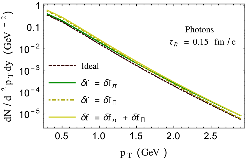
Similarly, we analyse the effect of dissipation on thermal photon yield in Figs. 9 and 10. Impact of viscous terms on photon yield is studied with fm/c in Fig. 9. As observed for dilepton (in Fig. 6), maximum enhancement to the yield due to bulk viscosity () is observed at small , where as increment due to shear correction () is significant at high . The combined effect of both () leads to the maximum enhancement over the entire . Moreover, we note that the yield in the presence of bulk viscous correction crosses the curve around GeV, where as in Fig. 6 (for dileptons), this cross-over was observed around GeV. Fig. 10 exhibits a comparison between thermal photon yields for different . It is observed that enhancement in the yield is seen to be marginal with and yield is greatest with .
Finally, in Figs. 11 and 12, we compare the thermal dilepton and photon yields obtained within this new second order hydrodynamics with that of a standard one given by Eqs. (20), (25) and (26). The yields are plotted for and with invariant mass GeV (for dileptons). It is clear that the spectra of dileptons and photons depend strongly on the interaction effects in the medium. The presence of these interaction terms in the yield expressions within EQPM suppresses the particle production throughout the regime. This is inline with the results of Ref. Chandra and Sreekanth (2017). In Fig. 11, we also plot the dilepton yield within EQPM by neglecting the interaction effects on invariant mass of dilepton i.e., in the limit . It can be seen that the dilepton production yield increases in this limit as shown by the results of Ref. Naik et al. (2022).


VI Summary
We have employed the recently developed second order dissipative hydrodynamics estimated within the effective fugacity quasiparticle model to study the thermal dilepton and photon production from QGP. In this study, we have used the non-equilibrium quark-antiquark distribution functions, up to first order in momenta, determined using the iterative CE type expansion of effective Boltzmann equation in the relaxation time approximation (RTA). The second order viscous hydrodynamic equations were solved for different temperature dependent relaxation times () within the D boost invariant expansion of QGP and the evolution has been compared with that obtained for a temperature independent constant value fm/c. It must be emphasized that, the choice of this constant value is arbitrary. We have incorporated the effect of shear and bulk viscosity coefficients through their respective relaxation times and , ensuring as demanded by RTA. The impact of shear and bulk viscous pressures was found to increase with increment in . By looking into the dynamical pressure anisotropy with various relaxation times, we found that cavitation scenarios can be present in the medium for small values of . Moreover, we obtained the limiting values of relaxation times by looking into fireball reheating scenarios. Our analysis indicate that relaxation time should not increase the constant value fm/c and temperature dependent value .
Further, using this causal hydrodynamic model, we explored the thermal dilepton and photon yields from prominent production sources in the presence of viscous modified distribution functions within longitudinal expansion of the QGP. This was done after calculating the thermal particle spectra by including the viscous modified single particle distribution functions. The effect of both shear and bulk corrections under this formalism is to enhance the dilepton and photon spectra. We also analyzed the impact of dissipation on yields by varying the value of invariant mass. Thermal dilepton and photon yields were studied for different temperature dependent and we found that maximum enhancement is observed for the largest value of considered. Our results also indicate that thermal dilepton and photon spectra in the presence of first order dissipative terms in the distribution function does not exhibit large corrections from the ideal case and is well behaved compared to the results using Grad’s method Bhatt et al. (2012); Bhalerao et al. (2014). We also did a comparative study of the spectra calculated within EQPM hydrodynamic framework with that obtained in the absence of mean field terms, by employing a standard relativistic hydrodynamics. Our study indicates that the presence of interaction terms in the yield expressions suppress the thermal dilepton and photon spectra throughout the range. In future, we would like to study thermal dilepton and photon production by employing this causal second order hydrodynamic framework in the presence of Chapman-Enskog type viscous corrections, up to second order in gradients Bhadury et al. (2021). Further, it will be interesting to do a quantitative analysis with ()-D hydrodynamics by varying the initial conditions. We leave these aspects for future study.
Acknowledgements
L. J. N. acknowledges the Department of Science and Technology, Government of India for the INSPIRE Fellowship. We thank the anonymous referees of this article for comments which led to the improvement of quality of the manuscript.
Appendix A Second Order Transport Coefficients
The second order transport coefficients appearing in the viscous evolution Eqs. (18) and (19) are obtained as Bhadury et al. (2021)
| (60) | ||||
| (61) |
| (62) | ||||
| (63) | ||||
| (64) |
where,
| (65) | ||||
| (66) | ||||
| (67) | ||||
| (68) | ||||
| (69) | ||||
| (70) | ||||
| (71) |
Thermodynamic integrals appearing in the second order transport coefficients are as shown below
| (72) | ||||
| (73) | ||||
| (74) | ||||
| (75) |
We note that, these thermodynamic integrals can be approximated and expressed in terms of polylogrithmic functions of order and argument , PolyLog as shown in Ref. Bhadury et al. (2021).
References
- Adams et al. (2005) John Adams et al. (STAR), “Experimental and theoretical challenges in the search for the quark gluon plasma: The STAR Collaboration’s critical assessment of the evidence from RHIC collisions,” Nucl. Phys. A 757, 102–183 (2005), arXiv:nucl-ex/0501009 .
- Adcox et al. (2005) K. Adcox et al. (PHENIX), “Formation of dense partonic matter in relativistic nucleus-nucleus collisions at RHIC: Experimental evaluation by the PHENIX collaboration,” Nucl. Phys. A 757, 184–283 (2005), arXiv:nucl-ex/0410003 .
- Arsene et al. (2005) I. Arsene et al. (BRAHMS), “Quark gluon plasma and color glass condensate at RHIC? The Perspective from the BRAHMS experiment,” Nucl. Phys. A 757, 1–27 (2005), arXiv:nucl-ex/0410020 .
- Back et al. (2005) B. B. Back et al. (PHOBOS), “The PHOBOS perspective on discoveries at RHIC,” Nucl. Phys. A 757, 28–101 (2005), arXiv:nucl-ex/0410022 .
- Jaiswal et al. (2021) Amaresh Jaiswal et al., “Dynamics of QCD matter — current status,” Int. J. Mod. Phys. E 30, 2130001 (2021), arXiv:2007.14959 [hep-ph] .
- Kovtun et al. (2005) P. Kovtun, Dan T. Son, and Andrei O. Starinets, “Viscosity in strongly interacting quantum field theories from black hole physics,” Phys. Rev. Lett. 94, 111601 (2005), arXiv:hep-th/0405231 .
- Romatschke and Romatschke (2019) Paul Romatschke and Ulrike Romatschke, Relativistic Fluid Dynamics In and Out of Equilibrium, Cambridge Monographs on Mathematical Physics (Cambridge University Press, 2019) arXiv:1712.05815 [nucl-th] .
- Hiscock and Lindblom (1983) W.A. Hiscock and L. Lindblom, “Stability and causality in dissipative relativistic fluids,” Annals Phys. 151, 466–496 (1983).
- Hiscock and Lindblom (1985) William A. Hiscock and Lee Lindblom, “Generic instabilities in first-order dissipative relativistic fluid theories,” Phys. Rev. D 31, 725–733 (1985).
- Geroch and Lindblom (1990) Robert P. Geroch and L. Lindblom, “Dissipative relativistic fluid theories of divergence type,” Phys. Rev. D 41, 1855 (1990).
- Bemfica et al. (2018) Fábio S. Bemfica, Marcelo M. Disconzi, and Jorge Noronha, “Causality and existence of solutions of relativistic viscous fluid dynamics with gravity,” Phys. Rev. D 98, 104064 (2018), arXiv:1708.06255 [gr-qc] .
- Hoult and Kovtun (2020) Raphael E. Hoult and Pavel Kovtun, “Stable and causal relativistic Navier-Stokes equations,” JHEP 06, 067 (2020), arXiv:2004.04102 [hep-th] .
- Biswas et al. (2022) Rajesh Biswas, Sukanya Mitra, and Victor Roy, “Is first-order relativistic hydrodynamics in a general frame stable and causal for arbitrary interactions?” Phys. Rev. D 106, L011501 (2022), arXiv:2202.08685 [nucl-th] .
- MÃŒller (1967) I. MÃŒller, “Zum paradoxon der wÀrmeleitungstheorie,” Zeitschrift fÃŒr Physik 198, 329–344 (1967).
- Israel and Stewart (1979) W. Israel and J.M. Stewart, “Transient relativistic thermodynamics and kinetic theory,” Annals Phys. 118, 341–372 (1979).
- Jaiswal and Roy (2016) Amaresh Jaiswal and Victor Roy, “Relativistic hydrodynamics in heavy-ion collisions: general aspects and recent developments,” Adv. High Energy Phys. 2016, 9623034 (2016), arXiv:1605.08694 [nucl-th] .
- Bhadury et al. (2021) Samapan Bhadury, Manu Kurian, Vinod Chandra, and Amaresh Jaiswal, “Second order relativistic viscous hydrodynamics within an effective description of hot QCD medium,” J. Phys. G 48, 105104 (2021), arXiv:2010.01537 [hep-ph] .
- Chandra and Ravishankar (2009) Vinod Chandra and V. Ravishankar, “Quasi-particle model for lattice QCD: Quark-gluon plasma in heavy ion collisions,” Eur. Phys. J. C 64, 63–72 (2009), arXiv:0812.1430 [nucl-th] .
- Chandra and Ravishankar (2011) Vinod Chandra and V. Ravishankar, “A quasi-particle description of - flavor lattice QCD equation of state,” Phys. Rev. D 84, 074013 (2011), arXiv:1103.0091 [nucl-th] .
- Mitra and Chandra (2018) Sukanya Mitra and Vinod Chandra, “Covariant kinetic theory for effective fugacity quasiparticle model and first order transport coefficients for hot QCD matter,” Phys. Rev. D 97, 034032 (2018), arXiv:1801.01700 [nucl-th] .
- Jaiswal (2013a) Amaresh Jaiswal, “Relativistic dissipative hydrodynamics from kinetic theory with relaxation time approximation,” Phys. Rev. C 87, 051901 (2013a), arXiv:1302.6311 [nucl-th] .
- Jaiswal (2013b) Amaresh Jaiswal, “Relativistic third-order dissipative fluid dynamics from kinetic theory,” Phys. Rev. C 88, 021903 (2013b), arXiv:1305.3480 [nucl-th] .
- Chandra and Sreekanth (2015) Vinod Chandra and V. Sreekanth, “Quark and gluon distribution functions in a viscous quark-gluon plasma medium and dilepton production via annihilation,” Phys. Rev. D 92, 094027 (2015), arXiv:1511.01208 [nucl-th] .
- Dusling and Lin (2008) Kevin Dusling and Shu Lin, “Dilepton production from a viscous QGP,” Nucl. Phys. A 809, 246–258 (2008), arXiv:0803.1262 [nucl-th] .
- Dusling (2010) Kevin Dusling, “Photons as a viscometer of heavy ion collisions,” Nucl. Phys. A 839, 70–77 (2010), arXiv:0903.1764 [nucl-th] .
- Bhatt and Sreekanth (2010) Jitesh R. Bhatt and V. Sreekanth, “Photon emission from out of equilibrium dissipative parton plasma,” Int. J. Mod. Phys. E 19, 299–306 (2010), arXiv:0901.1363 [hep-ph] .
- Bhatt et al. (2012) Jitesh R. Bhatt, Hiranmaya Mishra, and V. Sreekanth, “Cavitation and thermal dilepton production in QGP,” Nucl. Phys. A 875, 181–196 (2012), arXiv:1101.5597 [hep-ph] .
- Chaudhuri and Sinha (2011) A. K. Chaudhuri and Bikash Sinha, “Direct photon production from viscous QGP,” Phys. Rev. C 83, 034905 (2011), arXiv:1101.3823 [nucl-th] .
- Vujanovic et al. (2014) Gojko Vujanovic, Clint Young, Bjoern Schenke, Ralf Rapp, Sangyong Jeon, and Charles Gale, “Dilepton emission in high-energy heavy-ion collisions with viscous hydrodynamics,” Phys. Rev. C 89, 034904 (2014), arXiv:1312.0676 [nucl-th] .
- Vujanovic et al. (2018) Gojko Vujanovic, Gabriel S. Denicol, Matthew Luzum, Sangyong Jeon, and Charles Gale, “Investigating the temperature dependence of the specific shear viscosity of QCD matter with dilepton radiation,” Phys. Rev. C 98, 014902 (2018), arXiv:1702.02941 [nucl-th] .
- Torrieri et al. (2008) Giorgio Torrieri, Boris Tomasik, and Igor Mishustin, “Bulk Viscosity driven clusterization of quark-gluon plasma and early freeze-out in relativistic heavy-ion collisions,” Phys. Rev. C 77, 034903 (2008), arXiv:0707.4405 [nucl-th] .
- Fries et al. (2008) Rainer J. Fries, Berndt Muller, and Andreas Schafer, “Stress Tensor and Bulk Viscosity in Relativistic Nuclear Collisions,” Phys. Rev. C 78, 034913 (2008), arXiv:0807.4333 [nucl-th] .
- Rajagopal and Tripuraneni (2010) Krishna Rajagopal and Nilesh Tripuraneni, “Bulk Viscosity and Cavitation in Boost-Invariant Hydrodynamic Expansion,” JHEP 03, 018 (2010), arXiv:0908.1785 [hep-ph] .
- Bhatt et al. (2010) Jitesh R. Bhatt, Hiranmaya Mishra, and V. Sreekanth, “Thermal photons in QGP and non-ideal effects,” JHEP 11, 106 (2010), arXiv:1011.1969 [hep-ph] .
- Paquet et al. (2016) Jean-François Paquet, Chun Shen, Gabriel S. Denicol, Matthew Luzum, Björn Schenke, Sangyong Jeon, and Charles Gale, “Production of photons in relativistic heavy-ion collisions,” Phys. Rev. C 93, 044906 (2016), arXiv:1509.06738 [hep-ph] .
- Bhatt et al. (2011) Jitesh R. Bhatt, Hiranmaya Mishra, and V. Sreekanth, “Shear viscosity, cavitation and hydrodynamics at LHC,” Phys. Lett. B 704, 486–489 (2011), arXiv:1103.4333 [hep-ph] .
- Coquet et al. (2021) Maurice Coquet, Xiaojian Du, Jean-Yves Ollitrault, Soeren Schlichting, and Michael Winn, “Intermediate mass dileptons as pre-equilibrium probes in heavy ion collisions,” Phys. Lett. B 821, 136626 (2021), arXiv:2104.07622 [nucl-th] .
- Naik et al. (2021a) Lakshmi J. Naik, Sunil Jaiswal, K. Sreelakshmi, Amaresh Jaiswal, and V. Sreekanth, “Hydrodynamical attractor and thermal particle production in heavy-ion collision,” (2021a), arXiv:2107.08791 [hep-ph] .
- Naik et al. (2021b) Lakshmi J. Naik, Sunil Jaiswal, K. Sreelakshmi, Amaresh Jaiswal, and V. Sreekanth, “Analytical attractors and thermal particle spectra from quark-gluon plasma,” DAE Symp. Nucl. Phys. 65, 660–661 (2021b).
- Chandra and Sreekanth (2017) Vinod Chandra and V. Sreekanth, “Impact of momentum anisotropy and turbulent chromo-fields on thermal particle production in quark–gluon-plasma medium,” Eur. Phys. J. C 77, 427 (2017), arXiv:1602.07142 [nucl-th] .
- Naik et al. (2022) Lakshmi J. Naik, V. Sreekanth, Manu Kurian, and Vinod Chandra, “Thermal dilepton production in collisional hot QCD medium in the presence of chromo-turbulent fields,” J. Phys. G 49, 075103 (2022), arXiv:2003.13645 [hep-ph] .
- Prakash et al. (2021) Jai Prakash, Manu Kurian, Santosh K. Das, and Vinod Chandra, “Heavy quark transport in an anisotropic hot QCD medium: Collisional and Radiative processes,” Phys. Rev. D 103, 094009 (2021), arXiv:2102.07082 [hep-ph] .
- Bhalerao et al. (2014) Rajeev S. Bhalerao, Amaresh Jaiswal, Subrata Pal, and V. Sreekanth, “Relativistic viscous hydrodynamics for heavy-ion collisions: A comparison between the Chapman-Enskog and Grad methods,” Phys. Rev. C 89, 054903 (2014), arXiv:1312.1864 [nucl-th] .
- Cheng et al. (2008) M. Cheng et al., “The QCD equation of state with almost physical quark masses,” Phys. Rev. D 77, 014511 (2008), arXiv:0710.0354 [hep-lat] .
- Borsanyi et al. (2014) Szabocls Borsanyi, Zoltan Fodor, Christian Hoelbling, Sandor D. Katz, Stefan Krieg, and Kalman K. Szabo, “Full result for the QCD equation of state with 2+1 flavors,” Phys. Lett. B 730, 99–104 (2014), arXiv:1309.5258 [hep-lat] .
- Landau and Lifshitz (1987) L. D. Landau and E. M. Lifshitz, Fluid Mechanics, Vol. 6 (1987).
- Bjorken (1983) J. D. Bjorken, “Highly Relativistic Nucleus-Nucleus Collisions: The Central Rapidity Region,” Phys. Rev. D 27, 140–151 (1983).
- Baier et al. (2008) Rudolf Baier, Paul Romatschke, Dam Thanh Son, Andrei O. Starinets, and Mikhail A. Stephanov, “Relativistic viscous hydrodynamics, conformal invariance, and holography,” JHEP 04, 100 (2008), arXiv:0712.2451 [hep-th] .
- Natsuume and Okamura (2008) Makoto Natsuume and Takashi Okamura, “Causal hydrodynamics of gauge theory plasmas from AdS/CFT duality,” Phys. Rev. D 77, 066014 (2008), [Erratum: Phys.Rev.D 78, 089902 (2008)], arXiv:0712.2916 [hep-th] .
- York and Moore (2009) Mark Abraao York and Guy D. Moore, “Second order hydrodynamic coefficients from kinetic theory,” Phys. Rev. D 79, 054011 (2009), arXiv:0811.0729 [hep-ph] .
- Kanitscheider and Skenderis (2009) Ingmar Kanitscheider and Kostas Skenderis, “Universal hydrodynamics of non-conformal branes,” JHEP 04, 062 (2009), arXiv:0901.1487 [hep-th] .
- Srivastava (1999) Dinesh Kumar Srivastava, “Photon production in relativistic heavy ion collisions using rates with two loop calculations from quark matter,” Eur. Phys. J. C 10, 487–490 (1999), [Erratum: Eur.Phys.J.C 20, 399–400 (2001)], arXiv:nucl-th/0103023 .
- Muronga (2002) Azwinndini Muronga, “Second order dissipative fluid dynamics for ultrarelativistic nuclear collisions,” Phys. Rev. Lett. 88, 062302 (2002), [Erratum: Phys.Rev.Lett. 89, 159901 (2002)], arXiv:nucl-th/0104064 .
- Baier et al. (2006) Rudolf Baier, Paul Romatschke, and Urs Achim Wiedemann, “Dissipative hydrodynamics and heavy ion collisions,” Phys. Rev. C 73, 064903 (2006), arXiv:hep-ph/0602249 .
- Muronga (2004) Azwinndini Muronga, “Causal theories of dissipative relativistic fluid dynamics for nuclear collisions,” Phys. Rev. C 69, 034903 (2004), arXiv:nucl-th/0309055 .
- Alam et al. (1996) J. Alam, B. Sinha, and S. Raha, “Electromagnetic probes of quark gluon plasma,” Phys. Rept. 273, 243–362 (1996).
- Bhalerao et al. (2013) Rajeev S. Bhalerao, Amaresh Jaiswal, Subrata Pal, and V. Sreekanth, “Particle production in relativistic heavy-ion collisions: A consistent hydrodynamic approach,” Phys. Rev. C 88, 044911 (2013), arXiv:1305.4146 [nucl-th] .
- Wong (1995) C. Y. Wong, Introduction to high-energy heavy ion collisions (1995).
- Dusling and Teaney (2008) K. Dusling and D. Teaney, “Simulating elliptic flow with viscous hydrodynamics,” Phys. Rev. C 77, 034905 (2008), arXiv:0710.5932 [nucl-th] .
- Vogt (2007) Ramona Vogt, Ultrarelativistic heavy-ion collisions (Elsevier, Amsterdam, 2007).