Second MAYA Catalog of Binary Black Hole Numerical Relativity Waveforms
Abstract
Numerical relativity waveforms are a critical resource in the quest to deepen our understanding of the dynamics of, and gravitational waves emitted from, merging binary systems. We present 181 new numerical relativity simulations as the second MAYA catalog of binary black hole waveforms (a sequel to the Georgia Tech waveform catalog). Most importantly, these include 55 high mass ratio (), 48 precessing, and 92 eccentric () simulations, including 7 simulations which are both eccentric and precessing. With these significant additions, this new catalog fills in considerable gaps in existing public numerical relativity waveform catalogs. The waveforms presented in this catalog are shown to be convergent and are consistent with current gravitational wave models. They are available to the public at https://cgp.ph.utexas.edu/waveform.
I Introduction
Gravitational wave observations have become increasingly frequent, with the LIGO Scientific, Virgo and KAGRA Collaborations (LVK) reporting 90 detections through the end of their third observing run, including 83-85 likely binary black holes (BBHs) LIGO Scientific Collaboration, Virgo Collaboration, and KAGRA Collaboration (2021a); Abbott et al. (2021a, b, 2019), and more are expected in the fourth observing run. The BBH systems observed by the LVK span a large range of parameters, including mass ratios from equal mass to the possible 9:1 mass ratio of GW190814 LIGO Scientific Collaboration and Virgo Collaboration (2020). While most of the events are consistent with nonspinning black holes (BHs), some show evidence of strong precession LIGO Scientific Collaboration, Virgo Collaboration, and KAGRA Collaboration (2021a), and some events even show signs of eccentricity Gayathri et al. (2022); Romero-Shaw et al. (2021). As we prepare for next-generation gravitational-wave detectors such as the Laser Interferometer Space Antenna (LISA) Baker et al. (2019); Amaro-Seoane et al. (2017); Robson et al. (2019), the Einstein Telescope (ET) Punturo et al. (2010); Abernathy et al. (2011), and Cosmic Explorer (CE) Evans et al. (2021), we anticipate a significant increase in the volume of signals as well as a more diverse parameter space. Understanding the properties of the systems these signals come from and their underlying populations LIGO Scientific Collaboration and Virgo Collaboration (2021) and using the signals to test General Relativity (GR) LIGO Scientific Collaboration, Virgo Collaboration, and KAGRA Collaboration (2021b) relies upon having accurate predictions of the anticipated signals.
Due to the complex nature of Einstein’s theory of GR, analytic solutions don’t exist for the full two body problem of merging compact objects. A number of techniques have been developed to solve for the dynamics and radiation of such systems, and the most appropriate technique depends upon the parameters of the binary system in question. When the objects are far apart, post-Newtonian (PN) approximations can be used with high accuracy and confidence Isoyama et al. (2020); Blanchet (2014); Schäfer and Jaranowski (2018); Futamase and Itoh (2007); Blanchet et al. (2008); Faye et al. (2012, 2015). For systems where the masses of the black holes are highly unequal, small mass ratio approximations allow for efficient simulations Hinderer and Flanagan (2008); Miller and Pound (2021); Barack and Pound (2019). Great progress has also been made towards using small mass ratio approximations for the inspiral of near equal mass ratio systems van de Meent and Pfeiffer (2020); Wardell et al. (2021); Warburton et al. (2021); Albertini et al. (2022a, b).
In the highly nonlinear regime of the merger of comparably massed compact objects, numerical relativity (NR) is the most accurate approach. NR computationally solves Einstein’s equations by expressing them in a 3+1 formalism and separating the constraint and evolution equations in order to create an initial value problem that can be evolved on a computer Baumgarte and Shapiro (1998a, 2010, b). For the case of BBHs in vacuum, there is no missing physics within the simulations, as long as GR is correct, and the only limitations are computational in nature. A NR simulation will solve Einstein’s equations for a single binary system described by the masses and spin vectors of the two component BHs. For BBHs in vacuum, the results of the simulation can be scaled by the total mass, so we set the total ADM mass of the system to 1, and the masses can then simply be described by the mass ratio, . By creating template banks of NR simulations, NR waveforms have been used directly in gravitational wave (GW) detection and parameter estimation Lange et al. (2017); Abbott et al. (2016); Gayathri et al. (2022); Calderon Bustillo et al. (2022).
These simulations are placed discretely throughout the parameter space and are time consuming and computationally expensive. Therefore, while NR waveforms can be used directly as template banks for GW analysis, for many analyses, analytic or semi-analytic models are created, using information from NR for calibration Varma et al. (2019a); Bohé et al. (2017); Khan et al. (2016); Blackman et al. (2017); Husa et al. (2016); Taracchini et al. (2014); Hannam et al. (2014); Santamaria et al. (2010); Nakano et al. (2011); Pratten et al. (2021). However, creating reliable models and template banks relies upon NR waveforms being sufficiently accurate and densely covering the complete parameter space Ferguson et al. (2021); Pürrer and Haster (2020).
There are several NR codes and public waveform catalogs created by the NR community. The SXS collaboration has a public waveform catalog generated using their SpEC code Mroué et al. (2013); Boyle et al. (2019) and have been developing their next-generation code, SpECTRE Deppe et al. (2021). There are several waveform catalogs generated with codes derived from an open source software used by many NR groups Loffler et al. (2012), the Einstein Toolkit Jani et al. (2016); Healy et al. (2017a, 2019); Healy and Lousto (2022, 2020). The waveforms in the catalog presented in this paper are also generated with a code derived from the Einstein Toolkit, called Maya.
We previously released the Georgia Tech waveform catalog Jani et al. (2016) using our Maya code including 452 waveforms covering the spinning parameter space up to and including nonspinning waveforms up to . These waveforms have been used to study exceptional LVK events Lange et al. (2017), the detectability of intermediate-mass BHs Jani et al. (2019); Chandra et al. (2020); Abbott et al. (2022), as well as post-merger chirps Calderón Bustillo et al. (2019), to highlight a few recent studies. They have also been used to study the different stages of the merger, including finding a relationship between the frequency at merger and the spin of the remnant BH Ferguson et al. (2019); Healy et al. (2014). Using the Georgia Tech catalog, it was also found that the BH recoil can be measured from GW observations Calderón Bustillo et al. (2018), a method which has been applied to real events Calderón Bustillo et al. (2022). This catalog has since been rebranded to the MAYA Catalog.
This paper introduces the second MAYA Catalog, expanding beyond the parameter space coverage of the first catalog and introducing a new format. This format can be read using the mayawaves python library Ferguson et al. (2023a, b), which is described further in Section II.2. The new catalog includes a suite of eccentric simulations as well as improved coverage of the high mass ratio parameter space and the precessing parameter space. In Section II, we describe the Maya code used to create this catalog as well as the mayawaves python library. We then dive into the description of the new catalog in Section III. Section IV compares our simulations to other NR waveforms and waveform models, including an eccentric model, and Section V compares the models for the remnant BH parameters to the results obtained from our catalog. Finally, in Section VI, we include a discussion of the impact of center-of-mass (COM) drift corrections.
II Codebase
In this section, we’ll describe the code used to perform these NR simulations (Maya) as well as the python library used to interact with and analyze the simulations (mayawaves).
II.1 Maya Code
This catalog was constructed from simulations performed using the Maya code, a fork of the Einstein Toolkit using additional and modified thorns. The Einstein Toolkit is a finite-differencing code based upon the Cactus infrastructure using Carpet for box-in-box mesh refinement Schnetter et al. (2004). Maya uses the BSSN formulation Baumgarte and Shapiro (1998a) to separate Einstein’s equations into constraint equations to solve for the initial data and evolution equations to evolve the spacetime. The initial data consists of the extrinsic curvature and the spatial metric and is constructed using the TwoPunctures method Ansorg et al. (2004). The extrinsic curvature takes the Bowen-York form Bowen and York (1980), and the initial spacial metric is confomally flat. To set the initial momenta for quasi-circular simulations, we use the PN equations described in Healy et al. (2017b). We use the moving puncture gauge condition Campanelli et al. (2006); Baker et al. (2006) and use the Kranc scripts to generate the thorns for the spacetime evolution Husa et al. (2006).
The Weyl Scalar is computed throughout the computational domain (x,y,z), but to interpret it as gravitational radiation, it is extracted at several radii and extrapolated to spatial infinity. The waves are then decomposed and stored using the spin-weighted spherical harmonics as a basis:
| (1) |
where R is the extraction radius, M is the total mass of the binary, and and specify the location on the sphere centered at the COM of the binary. We provide the gravitational wave data at several extraction radii and mayawaves can be used to extrapolate the data to infinity using the method described in Lousto et al. (2010); Nakano et al. (2011). mayawaves also allows you to compute the strain, , which is related to by the following:
| (2) |
In our previous catalog paper, we showed that the Maya code is convergent Jani et al. (2016). Since this catalog introduces eccentric simulations, we include a convergence test for a simulation that is representative of the suite of included eccentric simulations. We consider a nonspinning system with and eccentricity, for three different resolutions, , , and . Figure 1(a) shows the residuals scaled by the factor , defined as:
| (3) |
where is the convergence rate which proves to be 2.36 for this simulation. We use 6-th order spacial finite differencing and 4th order Runge-Kutta for time evolution. Given the complex mesh refinement and the interpolation necessary to extract on spheres, this convergence rate is as expected.
We use the results from our convergence test to estimate the errors in our highest resolution waveform. Figure 1(b) shows the estimated error in our highest resolution waveform for this system. Based on the method presented in Ferguson et al. (2021), this will be indistinguishable from an “infinite” resolution face-on signal up to a signal-to-noise ratio (SNR) of .


II.2 mayawaves Python Library
The simulations in this catalog are provided in two formats. The more comprehensive format consists of an h5 file for each simulation that contains information relating to the compact objects as well as the radiation they emit. This h5 file should be read using the mayawaves python library Ferguson et al. (2023a, b). This library provides easy and efficient use of the MAYA catalog and can also be used to analyze any Einstein Toolkit simulation. Storing the simulations in this format enables us to provide more raw data pertaining to radiated quantities as well as the evolution of the compact objects themselves. The user need only download the desired waveform from our catalog, import mayawaves in their python file, and create a Coalescence object by passing in the simulation’s path to the constructor. They can then access all information regarding the simulation through the Coalescence object. The mayawaves library can be installed via pip or from source at https://github.com/MayaWaves/mayawaves. Documentation and tutorials can be found at https://mayawaves.github.io/mayawaves. Refer to Ferguson et al. (2023a) for more information on this library.
III Catalog Description
The MAYA catalog of NR waveforms is accessible at https://cgp.ph.utexas.edu/waveform. At that location, you will see a table with the metadata describing each simulation in the catalog. From that table, you can download each of the simulations. They are stored in an h5 format that is designed to be read using the mayawaves python library. Any simulations that contain all the necessary data are also provided in the format detailed in Schmidt et al. (2017) for use with PyCBC LIGO Scientific Collaboration (2018); Nitz et al. (2020).
This catalog introduces 181 new simulations that expand our coverage of the BBH parameter space, for a total of 635 simulations. The catalog website has also been updated to include the original catalog Jani et al. (2016) in the new mayawaves compatible format. Figure 2 shows the coverage of the previous catalog and this catalog, highlighting the many more eccentric simulations, precessing simulations, and high mass ratio simulations introduced by this catalog. Figure 3 shows the spin coverage of the combined catalogs. Figure 4 shows the distribution of the number of inspiral GW cycles after junk radiation for each simulation in the original and new catalogs. Simulations in the new catalog have a median of GW cycles and the overall catalog has a median of GW cycles.
This catalog is an amalgamation of several suites of simulations performed for various studies. This includes a suite of 80 non-precessing, eccentric simulations with mass ratios up to . It includes 38 simulations for a study of secondary spin for mass ratios up to . We also include 9 simulations performed for LVK followup studies. Finally we have 31 simulations placed to optimally fill in gaps in our parameter space using the network and method described in Ferguson (2022). Each of these suites is described in more detail below. The remaining 23 simulations are an assortment of simulations performed over the last few years.


III.1 Eccentric
As orbits evolve, eccentricity is quickly radiated away Peters (1964); therefore, for most scenarios, the eccentricity is expected to be minimal by the time a stellar mass BBH system reaches current ground-based GW detectors’ frequency bands. As a consequence, most NR simulations and GW models have focused on quasicircular binary systems. However, there are astrophysical situations that can lead to non-zero eccentricity in binaries observed by ground-based detectors Romero-Shaw et al. (2021); Samsing (2018); Rodriguez et al. (2018); Morscher et al. (2015); Zevin et al. (2019). Some future GW detectors such as LISA, will observe many binaries earlier in their inspiral and are expected to see some eccentricity remaining within the signals. In order to be prepared to detect and study these signals, we will need eccentric NR simulations and eccentric GW models. In fact, some LVK events have already shown potential evidence for eccentricity, increasing the urgency with which we need to explore this parameter space Gayathri et al. (2022); Romero-Shaw et al. (2021). As part of this catalog, we have included 92 new eccentric simulations.
80 of these simulations were part of a systematic suite designed to explore the eccentric space. They have mass ratios of by steps of 1, and for each , we have aligned with the orbital angular momentum. For each of the above cases, we performed simulations with eccentricity, by steps of These simulations have catalog ids of MAYA0913-MAYA0931, MAYA0938-MAYA0947, MAYA0949-MAYA0958, MAYA0960-MAYA0969, MAYA0971-MAYA0980, MAYA0982-MAYA1001, and MAYA1041. For each , , combination, the catalog also includes a quasicircular simulation.
Since eccentricity is a Newtonian concept, there is no unambiguous definition of eccentricity within GR. The mayawaves library currently uses the orbital frequency definition described in Ramos-Buades et al. (2019). This definition has proved to be robust and consistent with other definitions of eccentricity. For setting up the eccentric simulations, we use the method described in Gayathri et al. (2022), applying a Newtonian derived correction to the quasicircular momentum. Since this definition is based on Newtonian assumptions, the resulting eccentricities are not exactly the same as the target eccentricities. As we are aiming to generally fill out the eccentric space and do not need precise values of … , we do not apply iterative corrections to target the exact eccentricity values.
We also include 5 additional simulations with and eccentricities up to . These have catalog ids of MAYA0932-MAYA0936. Additionally, we have 7 simulations with both eccentricity and precession, with ids MAYA1043-MAYA1049. These are particularly useful since there are currently no eccentric, precessing waveform models.
III.2 Secondary Spin
We performed a suite of simulations spanning mass ratios of with varying spins, including 9 simulations with . The primary BH is nonspinning and the secondary BH has an aligned spin of by steps of 0.2. Current public NR catalogs have minimal coverage of the parameter space with , especially with secondary spin. These simulations help fill that gap. This suite also enables us to study the impact of the secondary spin as a function of mass ratio. The simulations with begin with a separation of and the simulations begin at . This suite includes simulations with ids MAYA1002-MAYA1039.
III.3 LVK Followup
Some of the detections made by the LVK have required additional NR followup. This is particularly useful for events that push to the edges of the regions where models are sufficiently trained or in situations where different models yield inconsistent posteriors for the parameters of the binary. We performed 7 simulations (MAYA1050-MAYA1056) as followup for GW190521, an event that has been the focus of a lot of different studies due to its limited number of cycles Gayathri et al. (2022); Romero-Shaw et al. (2021); Abbott et al. (2020); Gamba et al. (2023); Calderón Bustillo et al. (2021). By using RIFT to perform parameter estimation on GW190521 with NR simulations, these points in parameter space were identified as locations with both high likelihood and high uncertainty in the fit Lange et al. (2017). Performing simulations at these points and then repeating the RIFT analysis with the new waveforms included is expected to improve the accuracy of and confidence in the estimated parameters for GW190521. Also for GW190521, we performed a simulation at the point of maximum likelihood for the purpose of visualizations for the announcement of the first intermediate-mass BH observation. We also performed one simulation (MAYA0912) as followup for GW170608.
III.4 Optimized Template Placement
Many of our simulations are performed for specific studies and thus have very specific initial parameters. However, in order to prepare for future LVK runs and next-generation detectors, we also want to fill out our catalog in an efficient and strategic way. To accomplish this, we use the neural network presented in Ferguson (2022) and the method it describes to identify optimal parameters. This method makes use of a neural network trained to predict the match between any two quasi-circular binary systems given their initial parameters. Using this network, we search for the minimal match between potential simulations and those already existing in the catalog. Given the non-smooth nature of the space, we use basin hopping to identify global minima.
This tool has enabled us to identify and perform simulations in a way that maximally fills in gaps in our coverage. We have just begun to use this tool and have performed 31 simulations suggested by it, with ids MAYA1057-MAYA1087. These simulations have mass ratios up to and precessing spins up to magnitudes of . Current catalogs have dense coverage in low mass-ratio spaces, but have minimal coverage above . In general, the precessing space is also much less densely covered than the aligned spin space. These 31 simulations make significant improvements to the coverage of the moderate to high mass-ratio, precessing parameter space. This tool will play a large role in the generation of waveforms for our future catalogs.
IV Waveform Comparisons
Within the NR community, there are several different methods and techniques for solving Einstein’s equations directly. While each method has its benefits and drawbacks, all NR waveforms are considered to the be the gold standard for studying the merger of comparable-mass BBH systems. To ensure accuracy and consistency in analyses that use NR waveforms of each technique, it is important to perform cross-code comparisons. Several of these have been done over the past couple decades, and the methods used by the Einstein Toolkit and the Simulating eXtreme Spacetimes (SXS) Collaboration have proven to be reliable Ajith et al. (2012); Hinder et al. (2013); Healy et al. (2018). Here, we provide a comparison between this catalog and comparable waveforms available in the SXS catalog.
Similarly, there are many analytic and semi-analytic models for computing GWs. These models have the benefit of being faster than NR allowing for continuous sampling of the parameter space. However, given that these models are trained or calibrated to NR waveforms, they are generally not considered to be as accurate as NR waveforms. In this section we will also perform a comparison between this catalog and waveforms generated using such models.
For each of these comparisons, we compute the mismatch on a flat noise curve, defined as:
| (4) |
where
| (5) |
with being a flat PSD, and denoting the complex conjugate. Mismatches are very sensitive to systematic effects such as the amount of tapering and the starting frequency, and we find that these effects can change the mismatches by up to . For consistency and to reduce Gibbs oscillations, we consider only waveforms with more than 10 inspiral cycles and taper 6 of them. We compute all mismatches using a total mass of and a starting frequency of 30 Hz.
For the SXS comparison, we consider all equivalent non-precessing systems that exist in our catalog and in the SXS LVK catalog. Figure 5(a) shows the mismatch as a function of inclination, using all available modes and a flat noise curve. The grey lines show each individual system and the black line shows the median. Figure 5(b) shows the distribution of mismatches (including all 20 inclinations) with a median mismatch of .


We also compare our waveforms to the current state-of-the-art waveform models. For the quasicircular case, we compare to IMRPhenomXPHM Pratten et al. (2021) for both precessing and non-precessing systems, and for the eccentric case, we compare to TEOBResumS-DALI Chiaramello and Nagar (2020); Nagar et al. (2021); Nagar and Rettegno (2021); Placidi et al. (2022). Figure 6(a) shows the mismatch between the quasicircular NR waveforms and the IMRPhenomXPHM waveforms as a function of inclination, including all available modes on a flat noise curve. Each of the precessing systems appears as a faint orange line with the vibrant orange line showing the median value for all precessing simulations. All non-precessing simulations appear as faint blue lines with the vibrant blue line showing the median value for all non-precessing simulations. The black line shows the median mismatch of all quasicircular simulations. Figure 6(b) shows the distribution of the mismatches for precessing (blue) and aligned (orange) systems including 20 uniformly distributed inclinations. For non-precessing systems, the median mismatch is , and for the precessing systems, the median mismatch is .


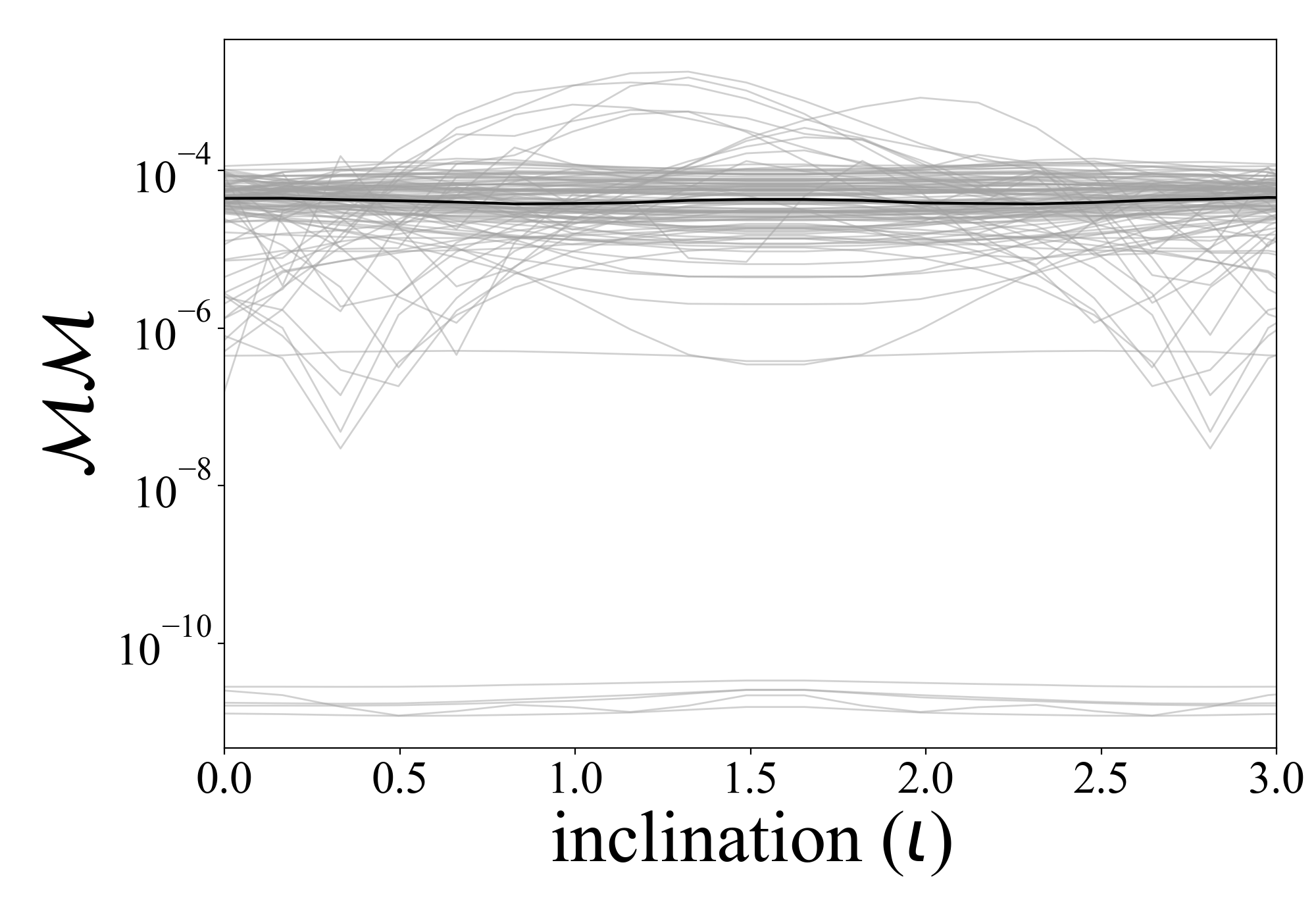
For the eccentric case, we use TEOBResumS-DALI as the waveform model and consider only aligned spin systems. We optimize over the initial eccentricity and frequency of the model waveforms to obtain the best mismatch, since the model’s eccentricity parameter is not physically meaningful. Figure 7 shows the mismatches between TEOBResumS-DALI waveforms and 20 of our waveforms which fall within the validity range of the model (, , and ). The median mismatch over all systems and inclinations is .


V Final Mass, Spin, and Kick
In this section, we compare the properties of the remnant BH computed from NR simulations to those predicted using NRSur7dq4Remnant Varma et al. (2019a). We use the SurfinBH python library Varma et al. (2019b, 2018) to interact with NRSur7dq4Remnant and compute the predicted remnant properties. We provide the masses and spins of the initial BHs at a time before merger, rotated into the same frame used by NRSur7dq4Remnant. We only consider systems which fall within the range of validity for NRSur7dq4Remnant ( and dimensionless spin parameters ). The masses and spins of the initial and remnant BHs are computed from the BH apparent horizons, and the magnitude of the kick velocity is computed from the linear momentum radiated by the GWs.


Figure 8 shows the remnant properties obtained from NR simulations compared to the remnant properties obtained from NRSur7dq4Remnant. For each of the remnant properties, the non-precessing systems have much lower errors than the precessing systems. However, for remnant spin, all residuals fall within , and for remnant mass, all residuals fall within . The recoil velocity is more challenging since it is very sensitive to spin angles. The system with the largest residual has an error of .
VI Center of Mass Drift Corrections
During the NR simulation of the inspiral of BBH systems, the center of mass experiences a wobble and a drift. These are caused by a combination of physical effects due to the asymmetrical emission of GWs and numerical error. Since the GWs are decomposed with the spherical harmonics centered on the initial COM, this can cause mode mixing. In recent years there has been much discussion of the impact that these COM drifts can cause to the waveform modes. We include here a brief analysis of the impact of correcting for such drifts.
Using the Scri python package Boyle et al. (2020); Boyle (2013); Boyle et al. (2014); Boyle (2016), we apply corrections for a translation and boost in the COM, computed using equations 6 and 7 of Woodford et al. (2019). We then perform a mismatch analysis comparing the COM corrected waveforms and the uncorrected waveforms for the overall strain and for individual modes. Figure 9 shows the mismatches between raw and COM corrected strains. In Figure 9(a), we see the mismatch with all modes combined as a function of inclination. The median mismatch is fairly constant for all inclinations, with a value of . In Figure 9(b), we see the mismatch values for several modes as a function of mass ratio. While there does not appear to be a strong correlation between the impact of COM corrections and mass ratio, the figure does reveal that certain modes are more impacted than others. In particular, the , mode has mismatches up to .

VII Conclusion
This paper introduces the second MAYA catalog of NR waveforms. It contains 181 waveforms that fill in and expand our coverage of the BBH parameter space. This includes 80 from an eccentric suite ranging up to eccentricities of 0.1, as well as 7 systems with both precession and eccentricity. It also includes 38 waveforms studying secondary spin, 9 simulations as NR followup for LVK events, and 31 simulations placed to optimize parameter space coverage.
As the most accurate way of studying the merger of comparably massed objects, NR waveforms are crucial for understanding the observations of current and next-generation GW detectors. We must, therefore, ensure we have sufficient NR coverage of the anticipated parameter space. This catalog makes significant strides towards this goal by pushing and filling in considerable gaps in existing NR coverage of the BBH parameter space. With mass ratios up to , highly precessing simulations, and an extensive eccentric suite, this catalog greatly improves the coverage of public NR catalogs.
By performing a thorough error analysis and comparison to other NR codes, we are confident in the accuracy and reliability of the waveforms presented in this catalog. Through a comparison to state-of-the-art GW models, we show consistency but also highlight the continuing need for NR waveforms particularly in the less well understood precessing space.
The waveforms are provided at https://cgp.ph.utexas.edu/waveform and can be read using the mayawaves python package.
We have also updated the previous Georgia Tech catalog to include more data by using the new format, leading to a total of 635 public waveforms.
All waveforms that fit the requirements are also provided in the format described in Schmidt et al. (2017) for use with PYCBC.
Acknowledgements
The catalog and analysis presented in this paper are possible due to grants NASA 80NSSC21K0900, NSF 2207780 and NSF 2114582. The computing resources necessary to perform the simulations in this catalog were provided by XSEDE PHY120016, TACC PHY20039, TACC NR-Catalog and TACC Template-Placement. This work was done by members of the Weinberg Institute and has an identifier of UTWI-32-2023.
References
- LIGO Scientific Collaboration, Virgo Collaboration, and KAGRA Collaboration (2021a) LIGO Scientific Collaboration, Virgo Collaboration, and KAGRA Collaboration (LIGO Scientific, VIRGO, KAGRA), (2021a), arXiv:2111.03606 [gr-qc] .
- Abbott et al. (2021a) R. Abbott et al. (LIGO Scientific, VIRGO), (2021a), arXiv:2108.01045 [gr-qc] .
- Abbott et al. (2021b) R. Abbott et al. (LIGO Scientific, Virgo), Phys. Rev. X 11, 021053 (2021b), arXiv:2010.14527 [gr-qc] .
- Abbott et al. (2019) B. P. Abbott et al. (LIGO Scientific, Virgo), Phys. Rev. X 9, 031040 (2019), arXiv:1811.12907 [astro-ph.HE] .
- LIGO Scientific Collaboration and Virgo Collaboration (2020) LIGO Scientific Collaboration and Virgo Collaboration (LIGO Scientific, Virgo), Astrophys. J. Lett. 896, L44 (2020), arXiv:2006.12611 [astro-ph.HE] .
- Gayathri et al. (2022) V. Gayathri, J. Healy, J. Lange, B. O’Brien, M. Szczepanczyk, I. Bartos, M. Campanelli, S. Klimenko, C. O. Lousto, and R. O’Shaughnessy, Nature Astron. 6, 344 (2022), arXiv:2009.05461 [astro-ph.HE] .
- Romero-Shaw et al. (2021) I. M. Romero-Shaw, P. D. Lasky, and E. Thrane, Astrophys. J. Lett. 921, L31 (2021), arXiv:2108.01284 [astro-ph.HE] .
- Baker et al. (2019) J. Baker et al., arXiv e-prints , arXiv:1907.06482 (2019), arXiv:1907.06482 [astro-ph.IM] .
- Amaro-Seoane et al. (2017) P. Amaro-Seoane et al., arXiv e-prints , arXiv:1702.00786 (2017), arXiv:1702.00786 [astro-ph.IM] .
- Robson et al. (2019) T. Robson, N. J. Cornish, and C. Liu, Classical and Quantum Gravity 36, 105011 (2019).
- Punturo et al. (2010) M. Punturo et al., Class. Quant. Grav. 27, 194002 (2010).
- Abernathy et al. (2011) M. Abernathy et al., EGO (2011).
- Evans et al. (2021) M. Evans et al., arXiv e-prints , arXiv:2109.09882 (2021), arXiv:2109.09882 [astro-ph.IM] .
- LIGO Scientific Collaboration and Virgo Collaboration (2021) LIGO Scientific Collaboration and Virgo Collaboration (LIGO Scientific, Virgo), Astrophys. J. Lett. 913, L7 (2021), arXiv:2010.14533 [astro-ph.HE] .
- LIGO Scientific Collaboration, Virgo Collaboration, and KAGRA Collaboration (2021b) LIGO Scientific Collaboration, Virgo Collaboration, and KAGRA Collaboration (LIGO Scientific, VIRGO, KAGRA), (2021b), arXiv:2112.06861 [gr-qc] .
- Isoyama et al. (2020) S. Isoyama, R. Sturani, and H. Nakano, (2020), 10.1007/978-981-15-4702-7_31-1, arXiv:2012.01350 [gr-qc] .
- Blanchet (2014) L. Blanchet, Living Rev. Rel. 17, 2 (2014), arXiv:1310.1528 [gr-qc] .
- Schäfer and Jaranowski (2018) G. Schäfer and P. Jaranowski, Living Rev. Rel. 21, 7 (2018), arXiv:1805.07240 [gr-qc] .
- Futamase and Itoh (2007) T. Futamase and Y. Itoh, Living Rev. Rel. 10, 2 (2007).
- Blanchet et al. (2008) L. Blanchet, G. Faye, B. R. Iyer, and S. Sinha, Class. Quant. Grav. 25, 165003 (2008), [Erratum: Class.Quant.Grav. 29, 239501 (2012)], arXiv:0802.1249 [gr-qc] .
- Faye et al. (2012) G. Faye, S. Marsat, L. Blanchet, and B. R. Iyer, Class. Quant. Grav. 29, 175004 (2012), arXiv:1204.1043 [gr-qc] .
- Faye et al. (2015) G. Faye, L. Blanchet, and B. R. Iyer, Class. Quant. Grav. 32, 045016 (2015), arXiv:1409.3546 [gr-qc] .
- Hinderer and Flanagan (2008) T. Hinderer and E. E. Flanagan, Phys. Rev. D 78, 064028 (2008), arXiv:0805.3337 [gr-qc] .
- Miller and Pound (2021) J. Miller and A. Pound, Phys. Rev. D 103, 064048 (2021), arXiv:2006.11263 [gr-qc] .
- Barack and Pound (2019) L. Barack and A. Pound, Rept. Prog. Phys. 82, 016904 (2019), arXiv:1805.10385 [gr-qc] .
- van de Meent and Pfeiffer (2020) M. van de Meent and H. P. Pfeiffer, Phys. Rev. Lett. 125, 181101 (2020), arXiv:2006.12036 [gr-qc] .
- Wardell et al. (2021) B. Wardell, A. Pound, N. Warburton, J. Miller, L. Durkan, and A. Le Tiec, (2021), arXiv:2112.12265 [gr-qc] .
- Warburton et al. (2021) N. Warburton, A. Pound, B. Wardell, J. Miller, and L. Durkan, Phys. Rev. Lett. 127, 151102 (2021), arXiv:2107.01298 [gr-qc] .
- Albertini et al. (2022a) A. Albertini, A. Nagar, A. Pound, N. Warburton, B. Wardell, L. Durkan, and J. Miller, Phys. Rev. D 106, 084061 (2022a), arXiv:2208.01049 [gr-qc] .
- Albertini et al. (2022b) A. Albertini, A. Nagar, A. Pound, N. Warburton, B. Wardell, L. Durkan, and J. Miller, Phys. Rev. D 106, 084062 (2022b), arXiv:2208.02055 [gr-qc] .
- Baumgarte and Shapiro (1998a) T. W. Baumgarte and S. L. Shapiro, Phys. Rev. D 59, 024007 (1998a), arXiv:gr-qc/9810065 .
- Baumgarte and Shapiro (2010) T. W. Baumgarte and S. L. Shapiro, Numerical Relativity: Solving Einstein’s Equations on the Computer (Cambridge University Press, 2010).
- Baumgarte and Shapiro (1998b) T. W. Baumgarte and S. L. Shapiro, Phys. Rev. D 59, 024007 (1998b).
- Lange et al. (2017) J. Lange et al., Phys. Rev. D 96, 104041 (2017), arXiv:1705.09833 [gr-qc] .
- Abbott et al. (2016) B. P. Abbott et al. (LIGO Scientific, Virgo), Phys. Rev. D 94, 064035 (2016), arXiv:1606.01262 [gr-qc] .
- Calderon Bustillo et al. (2022) J. Calderon Bustillo, N. Sanchis-Gual, S. H. W. Leong, K. Chandra, A. Torres-Forne, J. A. Font, C. Herdeiro, E. Radu, I. C. F. Wong, and T. G. F. Li, (2022), arXiv:2206.02551 [gr-qc] .
- Varma et al. (2019a) V. Varma, S. E. Field, M. A. Scheel, J. Blackman, D. Gerosa, L. C. Stein, L. E. Kidder, and H. P. Pfeiffer, Phys. Rev. Research. 1, 033015 (2019a), arXiv:1905.09300 [gr-qc] .
- Bohé et al. (2017) A. Bohé et al., Phys. Rev. D 95, 044028 (2017), arXiv:1611.03703 [gr-qc] .
- Khan et al. (2016) S. Khan, S. Husa, M. Hannam, F. Ohme, M. Pürrer, X. Jiménez Forteza, and A. Bohé, Phys. Rev. D 93, 044007 (2016), arXiv:1508.07253 [gr-qc] .
- Blackman et al. (2017) J. Blackman, S. E. Field, M. A. Scheel, C. R. Galley, C. D. Ott, M. Boyle, L. E. Kidder, H. P. Pfeiffer, and B. Szilágyi, Phys. Rev. D 96, 024058 (2017), arXiv:1705.07089 [gr-qc] .
- Husa et al. (2016) S. Husa, S. Khan, M. Hannam, M. Pürrer, F. Ohme, X. Jiménez Forteza, and A. Bohé, Phys. Rev. D 93, 044006 (2016), arXiv:1508.07250 [gr-qc] .
- Taracchini et al. (2014) A. Taracchini et al., Phys. Rev. D 89, 061502 (2014), arXiv:1311.2544 [gr-qc] .
- Hannam et al. (2014) M. Hannam, P. Schmidt, A. Bohé, L. Haegel, S. Husa, F. Ohme, G. Pratten, and M. Pürrer, Phys. Rev. Lett. 113, 151101 (2014), arXiv:1308.3271 [gr-qc] .
- Santamaria et al. (2010) L. Santamaria et al., Phys. Rev. D 82, 064016 (2010), arXiv:1005.3306 [gr-qc] .
- Nakano et al. (2011) H. Nakano, Y. Zlochower, C. O. Lousto, and M. Campanelli, Phys. Rev. D 84, 124006 (2011), arXiv:1108.4421 [gr-qc] .
- Pratten et al. (2021) G. Pratten et al., Phys. Rev. D 103, 104056 (2021), arXiv:2004.06503 [gr-qc] .
- Ferguson et al. (2021) D. Ferguson, K. Jani, P. Laguna, and D. Shoemaker, Phys. Rev. D 104, 044037 (2021), arXiv:2006.04272 [gr-qc] .
- Pürrer and Haster (2020) M. Pürrer and C.-J. Haster, Phys. Rev. Res. 2, 023151 (2020), arXiv:1912.10055 [gr-qc] .
- Mroué et al. (2013) A. H. Mroué et al., Physical Review Letters 111, 241104 (2013), arXiv:1304.6077 [gr-qc] .
- Boyle et al. (2019) M. Boyle et al., Classical and Quantum Gravity 36, 195006 (2019), arXiv:1904.04831 [gr-qc] .
- Deppe et al. (2021) N. Deppe, W. Throwe, L. E. Kidder, N. L. Fischer, F. Hébert, J. Moxon, C. Armaza, G. S. Bonilla, P. Kumar, G. Lovelace, E. O’Shea, H. P. Pfeiffer, M. A. Scheel, S. A. Teukolsky, I. Anantpurkar, M. Boyle, F. Foucart, M. Giesler, J. S. Guo, D. A. B. Iozzo, Y. Kim, I. Legred, D. Li, A. Macedo, D. Melchor, M. Morales, K. C. Nelli, T. Ramirez, H. R. Rüter, J. Sanchez, S. Thomas, N. A. Wittek, and T. Wlodarczyk, “Spectre,” (2021).
- Loffler et al. (2012) F. Loffler et al., Class. Quant. Grav. 29, 115001 (2012), arXiv:1111.3344 [gr-qc] .
- Jani et al. (2016) K. Jani, J. Healy, J. A. Clark, L. London, P. Laguna, and D. Shoemaker, Class. Quant. Grav. 33, 204001 (2016), arXiv:1605.03204 [gr-qc] .
- Healy et al. (2017a) J. Healy, C. O. Lousto, Y. Zlochower, and M. Campanelli, Class. Quant. Grav. 34, 224001 (2017a), arXiv:1703.03423 [gr-qc] .
- Healy et al. (2019) J. Healy, C. O. Lousto, J. Lange, R. O’Shaughnessy, Y. Zlochower, and M. Campanelli, Phys. Rev. D 100, 024021 (2019), arXiv:1901.02553 [gr-qc] .
- Healy and Lousto (2022) J. Healy and C. O. Lousto, Phys. Rev. D 105, 124010 (2022), arXiv:2202.00018 [gr-qc] .
- Healy and Lousto (2020) J. Healy and C. O. Lousto, Phys. Rev. D 102, 104018 (2020).
- Jani et al. (2019) K. Jani, D. Shoemaker, and C. Cutler, Nature Astron. 4, 260 (2019), arXiv:1908.04985 [gr-qc] .
- Chandra et al. (2020) K. Chandra, V. Gayathri, J. C. Bustillo, and A. Pai, Phys. Rev. D 102, 044035 (2020).
- Abbott et al. (2022) R. Abbott et al. (LIGO Scientific, VIRGO, KAGRA), Astron. Astrophys. 659, A84 (2022), arXiv:2105.15120 [astro-ph.HE] .
- Calderón Bustillo et al. (2019) J. Calderón Bustillo, C. Evans, J. A. Clark, G. Kim, P. Laguna, and D. Shoemaker, (2019), 10.1038/s42005-020-00446-7, arXiv:1906.01153 [gr-qc] .
- Ferguson et al. (2019) D. Ferguson, S. Ghonge, J. A. Clark, J. Calderon Bustillo, P. Laguna, D. Shoemaker, and J. Calderon Bustillo, Phys. Rev. Lett. 123, 151101 (2019), arXiv:1905.03756 [gr-qc] .
- Healy et al. (2014) J. Healy, P. Laguna, and D. Shoemaker, Class. Quant. Grav. 31, 212001 (2014), arXiv:1407.5989 [gr-qc] .
- Calderón Bustillo et al. (2018) J. Calderón Bustillo, J. A. Clark, P. Laguna, and D. Shoemaker, Phys. Rev. Lett. 121, 191102 (2018).
- Calderón Bustillo et al. (2022) J. Calderón Bustillo, S. H. W. Leong, and K. Chandra, (2022), arXiv:2211.03465 [gr-qc] .
- Ferguson et al. (2023a) D. Ferguson et al., (2023a), arXiv:2309.00653 [astro-ph.IM] .
- Ferguson et al. (2023b) D. Ferguson, S. Anne, M. Gracia-Linares, H. Iglesias, A. Jan, E. Martinez, L. Lu, F. Meoni, R. Nowicki, M. Trostel, B.-J. Tsao, and F. Valorz, “mayawaves,” (2023b).
- Schnetter et al. (2004) E. Schnetter, S. H. Hawley, and I. Hawke, Class. Quant. Grav. 21, 1465 (2004), arXiv:gr-qc/0310042 [gr-qc] .
- Ansorg et al. (2004) M. Ansorg, B. Bruegmann, and W. Tichy, Phys. Rev. D 70, 064011 (2004), arXiv:gr-qc/0404056 .
- Bowen and York (1980) J. M. Bowen and J. W. York, Phys. Rev. D 21, 2047 (1980).
- Healy et al. (2017b) J. Healy, C. O. Lousto, H. Nakano, and Y. Zlochower, Class. Quant. Grav. 34, 145011 (2017b), arXiv:1702.00872 [gr-qc] .
- Campanelli et al. (2006) M. Campanelli, C. O. Lousto, P. Marronetti, and Y. Zlochower, Phys. Rev. Lett. 96, 111101 (2006).
- Baker et al. (2006) J. G. Baker, J. Centrella, D.-I. Choi, M. Koppitz, and J. van Meter, Phys. Rev. Lett. 96, 111102 (2006), gr-qc/0511103 .
- Husa et al. (2006) S. Husa, I. Hinder, and C. Lechner, Computer Physics Communications 174, 983 (2006), gr-qc/0404023 .
- Lousto et al. (2010) C. O. Lousto, H. Nakano, Y. Zlochower, and M. Campanelli, Phys. Rev. D 82, 104057 (2010), arXiv:1008.4360 [gr-qc] .
- Schmidt et al. (2017) P. Schmidt, I. W. Harry, and H. P. Pfeiffer, (2017), arXiv:1703.01076 [gr-qc] .
- LIGO Scientific Collaboration (2018) LIGO Scientific Collaboration, “LIGO Algorithm Library - LALSuite,” free software (GPL) (2018).
- Nitz et al. (2020) A. Nitz, I. Harry, D. Brown, C. M. Biwer, J. Willis, T. D. Canton, C. Capano, L. Pekowsky, T. Dent, A. R. Williamson, S. De, G. Davies, M. Cabero, D. Macleod, B. Machenschalk, S. Reyes, P. Kumar, T. Massinger, F. Pannarale, dfinstad, M. Tápai, S. Fairhurst, S. Khan, L. Singer, S. Kumar, A. Nielsen, shasvath, idorrington92, A. Lenon, and H. Gabbard, “gwastro/pycbc: Pycbc release v1.15.4,” (2020).
- Ferguson (2022) D. Ferguson, (2022), arXiv:2209.15144 [gr-qc] .
- Peters (1964) P. C. Peters, Phys. Rev. 136, B1224 (1964).
- Samsing (2018) J. Samsing, Phys. Rev. D 97, 103014 (2018).
- Rodriguez et al. (2018) C. L. Rodriguez, P. Amaro-Seoane, S. Chatterjee, and F. A. Rasio, Phys. Rev. Lett. 120, 151101 (2018).
- Morscher et al. (2015) M. Morscher, B. Pattabiraman, C. Rodriguez, F. A. Rasio, and S. Umbreit, The Astrophysical Journal 800, 9 (2015).
- Zevin et al. (2019) M. Zevin, J. Samsing, C. Rodriguez, C.-J. Haster, and E. Ramirez-Ruiz, The Astrophysical Journal 871, 91 (2019).
- Ramos-Buades et al. (2019) A. Ramos-Buades, S. Husa, and G. Pratten, Phys. Rev. D 99, 023003 (2019), arXiv:1810.00036 [gr-qc] .
- Abbott et al. (2020) R. Abbott et al. (LIGO Scientific, Virgo), Phys. Rev. Lett. 125, 101102 (2020), arXiv:2009.01075 [gr-qc] .
- Gamba et al. (2023) R. Gamba, M. Breschi, G. Carullo, S. Albanesi, P. Rettegno, S. Bernuzzi, and A. Nagar, Nature Astron. 7, 11 (2023), arXiv:2106.05575 [gr-qc] .
- Calderón Bustillo et al. (2021) J. Calderón Bustillo, N. Sanchis-Gual, A. Torres-Forné, J. A. Font, A. Vajpeyi, R. Smith, C. Herdeiro, E. Radu, and S. H. W. Leong, Phys. Rev. Lett. 126, 081101 (2021), arXiv:2009.05376 [gr-qc] .
- Ajith et al. (2012) P. Ajith et al., Classical and Quantum Gravity 29, 124001 (2012), arXiv:1201.5319 [gr-qc] .
- Hinder et al. (2013) I. Hinder et al., Classical and Quantum Gravity 31, 025012 (2013), arXiv:1307.5307 [gr-qc] .
- Healy et al. (2018) J. Healy et al., Phys. Rev. D 97, 064027 (2018), arXiv:1712.05836 [gr-qc] .
- Chiaramello and Nagar (2020) D. Chiaramello and A. Nagar, Phys. Rev. D 101, 101501 (2020), arXiv:2001.11736 [gr-qc] .
- Nagar et al. (2021) A. Nagar, A. Bonino, and P. Rettegno, Phys. Rev. D 103, 104021 (2021), arXiv:2101.08624 [gr-qc] .
- Nagar and Rettegno (2021) A. Nagar and P. Rettegno, Phys. Rev. D 104, 104004 (2021), arXiv:2108.02043 [gr-qc] .
- Placidi et al. (2022) A. Placidi, S. Albanesi, A. Nagar, M. Orselli, S. Bernuzzi, and G. Grignani, Phys. Rev. D 105, 104030 (2022), arXiv:2112.05448 [gr-qc] .
- Varma et al. (2019b) V. Varma, D. Gerosa, L. C. Stein, F. Hébert, and H. Zhang, Phys. Rev. Lett. 122, 011101 (2019b), arXiv:1809.09125 [gr-qc] .
- Varma et al. (2018) V. Varma, L. C. Stein, and D. Gerosa, “vijayvarma392/surfinBH: Surrogate Final BH properties,” (2018).
- Boyle et al. (2020) M. Boyle, D. Iozzo, and L. C. Stein, “moble/scri: v1.2,” (2020).
- Boyle (2013) M. Boyle, Phys. Rev. D 87, 104006 (2013).
- Boyle et al. (2014) M. Boyle, L. E. Kidder, S. Ossokine, and H. P. Pfeiffer, “Gravitational-wave modes from precessing black-hole binaries,” (2014), arXiv:1409.4431 [gr-qc] .
- Boyle (2016) M. Boyle, Phys. Rev. D 93, 084031 (2016).
- Woodford et al. (2019) C. J. Woodford, M. Boyle, and H. P. Pfeiffer, Phys. Rev. D 100, 124010 (2019), arXiv:1904.04842 [gr-qc] .