Searching for Integrated Sachs-Wolfe Effect from Fermi-LAT Diffuse -ray Map
Abstract
In this paper, we estimate the cross-correlation power spectra between the Planck 2018 cosmic microwave background (CMB) temperature anisotropy map and the unresolved -ray background (UGRB) from the 9-years Fermi-Large Area Telescope (LAT) data. In this analysis, we use up to nine energy bins over a wide energy range of [0.631, 1000] GeV from the Fermi-LAT UGRB data. Firstly, we find that the Fermi data with the energy ranges [1.202, 2.290] GeV and [17.38, 36.31] GeV show the positive evidence for the Integrated Sachs-Wolfe (ISW) effect at confidence level, and the significance would be increased to when using these two energy bins together. Secondly, we apply the single power-law model to normalize the amplitude and use all the nine Fermi energy bins to measure the significance of the ISW effect, we obtained ( C.L.). For the robustness test, we implement a null hypothesis by randomizing the Fermi mock maps of nine energy bins and obtain the non-detection of ISW effect, which confirms that the ISW signal comes from the Fermi-LAT diffuse -ray data and is consistent with the standard CDM model prediction essentially. We use a cross-correlation coefficient to show the relation between different energy bins. Furthermore, we vary the cut ranges of galactic plane on the mask of Fermi map and carefully check the consequent influence on the ISW signal detection.
1 Introduction
The nature of dark energy is one of the most important question in the modern cosmology. As we know, dark energy is a predominated ingredient of the Universe, which takes 68% of the whole constituents (Aghanim et al., 2018). Measurements of the baryon acoustic oscillation (Eisenstein et al., 2005), distant Type Ia supernovae (Riess et al., 2004) and gravitational lensing (Bacon et al., 2000) give a good explanation and evidence that dark energy drives the acceleration of the Universe and the standard CDM theory can successful explain these observations very well. Furthermore, Cosmic Microwave Background (CMB) as a landmark in Big Bang cosmology theory, is a crucial measurement for many open problems. Besides, the CMB anisotropies which produced at very early times, have several important secondary effects, such as the CMB lensing and the Sunyaev-Zel’dovich effects, which could contribute additional anisotropies on the temperature of CMB photons.
The integrated Sachs-Wolfe effect (ISW; Sachs and Wolfe (1967)) is also one of the CMB secondary anisotropies, which is caused by cumulative effect of photons travel from the changing of the gravitational potentials after the recombination epoch. When a CMB photon falls into a gravitational potential well, it gains energy, while it loses energy when it climbs out. These effects would be cancelled if the potential is time independent, such as the matter dominated era in which the gravitational potential stays constant. However, when dark energy or curvature become important at later times, the potential evolves as the photon passes through it. In this case, additional CMB anisotropies will be produced. Therefore, observing the late-time ISW can be a powerful way to probe dark energy and its evolution.
However, the most significant ISW effect contributes to the CMB anisotropies on large scales that are strongly affected by the cosmic variance, which means it is quite challenging to directly extract the ISW information from the CMB observation. Fortunately, this problem can be solved by cross-correlating ISW temperature fluctuation and the density of astrophysical objects like galaxies (Crittenden and Turok, 1996). Such cross-correlation analysis has been already implemented in the literatures to detect the ISW effect. For the first detection, Crittenden and Turok (1996) and Boughn et al. (1998) have measured the cross-correlation of High Energy Astronomy Observatory (HEAO) X-ray data and CMB anisotropies from Cosmic Background Explorer (COBE), they claimed it is potential that the ISW effect as an important observation to confront the structures of the Universe. Afterwards, a similar set of analyses have been carried out which relied on CMB data from the Wilkinson Microwave Anisotropy Probe (WMAP) satellite and a variety of large scale structure (LSS) probes, such as the Two-Micron All-Sky Survey galaxy (2MASS) (Afshordi et al., 2004; Francis and Peacock, 2010; Dupe et al., 2011), the NRAO VLA Sky Survey (NVSS) radio galaxies (Nolta et al., 2004), galaxies from Sloan Digital Sky Survey (SDSS) (Scranton et al., 2003; Fosalba et al., 2003; Granett et al., 2008; Chen and Schwarz, 2016), the Wide-field Infrared Survey Explorer (WISE) survey (Goto et al., 2012; Ferraro et al., 2015), and the X-ray background HEAO catalogue (Boughn et al., 2002; Boughn and Crittenden, 2004). Furthermore, Giannantonio et al. (2008); Xia et al. (2011); Khosravi et al. (2016) have combined all these measurements together to detect the ISW effect with very high significance. Recently, based on current Planck data release, Ade et al. (2014) used the different methods gave the significance of detection ranges from 2 to 4; the detection level achieved at 3 in Ade et al. (2016) by combining the cross-correlation signal coming from all the galaxy catalogues; Stölzner et al. (2018) also combined various LSS tracer data sets in the radio, optical and infrared wavelength, and obtained more than detection of the ISW effect.
In our previous works (Camera et al., 2015; Cuoco et al., 2015; Regis et al., 2015; Xia et al., 2015; Tröster et al., 2016; Cuoco et al., 2017; Branchini et al., 2017; Colavincenzo et al., 2020; Tan and Colavincenzo, 2019), we have studied that gamma-ray maps of the Unresolved -ray background (UGRB) from Fermi-Large Area Telescope (LAT) data and cross-correlated with different catalogs of galaxies. We observed significant correlation after properly removing various contamination, which means that the UGRB from Fermi data could be a nice LSS tracer and, therefore, has the potential to search for the ISW effect. Therefore, here we use the UGRB from Fermi-LAT 9-year Pass 8 data release and the Planck 2018 temperature anisotropies to detect the ISW effect. This paper is structured as follows: in section 2, we introduce the data set we use; theoretical formulae are present in section 3; sections 4 and 5 give numerical results and some systematic checks; final summary is listed in section 6.
2 Data Sets
In this section, we briefly describe the CMB map from Planck satellite and -ray maps of the UGRB from the Fermi-LAT mission used in the analysis.
2.1 CMB Information
The CMB data we used comes from the Planck2018 full-mission data release (“PR3”) that are accessible on the Planck Legacy Archive (PLA111http://pla.esac.esa.int/pla). There are four methodologies (COMMANDER, SEVEM, SMICA, NILC) adopted to do the component-separation algorithms for maps and we choose the SMICA synthesized CMB map, which uses spectral matching technology (Akrami et al., 2018). Since the contribution of the ISW signal is mainly from large scales, usually we only need to use the maps with relative low resolution format, like or 128.
In this work, in order to avoid some extra uncertainties during degradation of Fermi maps, here we use the Planck map with to match the default format of Fermi maps we have generated, which shown in the first panel of Fig. 1. Concerning the strong contamination from the galactic foreground and confident point-sources, in the second panel of Fig. 1 we also show the temperature analysis mask provided by the Planck team which leaves about of the sky.


2.2 Fermi-LAT UGRB Maps
The Fermi-LAT is the pair-conversion -ray telescope with the high sensitivity to -rays in the high energy range from 20 MeV to 1 TeV for all-sky area. During 10 years of operation, it has been provided massive data for researches of the astrophysical sources, cosmic rays and UGRB, and so on. The Fermi-LAT collaboration has also produced several generations of high-energy -ray source catalogues over many years, including active galactic nuclei, pulsars and other kinds of extra-galactic and galactic sources.
In this work, we use the photon flux intensity maps in 9 energy bins (see Table. 1) from 631 MeV to 1 TeV over 108 months. The flux map is obtained from dividing the photon count maps by the exposure maps and the pixel area, and these corresponding exposure and count maps are directly produced by using the LAT Fermi tools v10r0p5222https://fermi.gsfc.nasa.gov/ssc/data/analysis/documentation/Cicerone/. The event class is selected from the Pass 8 ULTRACLEANVETO, which provides lower background contamination at low energies. Since the observed data has an energy dependent angular resolution of the instrument, to balance the point-spread function (PSF) and photon statistics, PSF3 and PSF1+2+3 events are used for the first bin and the rest of eight bins, respectively. The PSF is computed running the routine gtpsf from the Fermi-LAT Science Tools and legendre transform to window beam function to correct our analysis.
For the masks, we removed the contributions from the resolved sources list of 4FGL and 3FHL catalogs above 9 GeV. The 4FGL catalog is updated from the -ray sky with respect to 3FGL and has exposure twice longer, and contains nearly 5065 sources above significance. The 3FHL catalog, the third catalog of hard Fermi-LAT sources, contains 1556 objects characterized in the energy range [10, 2000] GeV.
This catalog was constructed by the first 7 years of data, and is updated by implementing improvements provided by the Pass 8 data. The radius is considered by the PSF for a gaussian method according to the containment angle. To reduce the impact of the Galactic emission on our analysis and focused on the UGRB, we apply a Galactic latitude cut , which represents the best compromise between pixel statistics and Galactic contamination, found in Xia et al. (2011), in order to mask the bright emission along the Galactic plane.
All the flux maps are in the same format with the Planck CMB map as described above with , containing pixels with space in each pixel. The foreground contamination is rejected by the Galactic emission model gll_iem_v06.fits333https://fermi.gsfc.nasa.gov/ssc/data/access/lat/BackgroundModels.html, which is provided by Fermi-LAT Collaboration in same number for the high-latitudes. One example map shows in Fig. 2, here we consider the -ray maps as continuous field on the celestial sphere, we access the density number of photons per map of one energy bin showed in table 1.

| Bin | [GeV] | [GeV] | Photon number density |
|---|---|---|---|
| [ph/] | |||
| 1 | 0.631 | 1.202 | 15.24 |
| 2 | 1.202 | 2.290 | 17.36 |
| 3 | 2.290 | 4.786 | 15.29 |
| 4 | 4.786 | 9.120 | 7.74 |
| 5 | 9.120 | 17.38 | 4.12 |
| 6 | 17.38 | 36.31 | 2.50 |
| 7 | 36.31 | 69.18 | 0.80 |
| 8 | 69.18 | 131.8 | 0.28 |
| 9 | 131.8 | 1000 | 0.037 |
3 Theoretical formalism
Following Xia et al. (2015), the cross-correlation power spectrum between -ray maps and CMB temperature anisotropic map can be easily obtained by,
| (1) |
where is the wavenumber, is the matter power spectrum at present time, and are the window functions for -ray and CMB observations, respectively. In the following, we derive the cross-correlation power spectrum by adopting the standard general relativity in the flat CDM framework. While the ISW effect for non-zero curvature or modified gravity, please refer to some previous studies (Kamionkowski, 1996; Song et al., 2007).
For the temperature fluctuations from CMB maps, the ISW signal in real space can be written as
| (2) |
where is the gravitational potential and represents the comoving distance. Here, we neglect a optical depth factor of , which would not affect our results because of the tiny modification when comparing with the typical accuracy achieved in the determination of the ISW effect itself. Using the Poisson equation, we have
| (3) |
where is the speed of light, is the cosmological scale factor, is the Hubble parameter at present time, is the fractional density of matter today, and is the matter fluctuation field in Fourier space. Finally we can obtain
| (4) |
where is the linear growth factor of density fluctuation, represent spherical Bessel functions, and is the mean temperature of the CMB photons at present.
We presume the variations that the number density of unresolved sources are responsible for the local fluctuation in the -ray luminosity density, . Therefore, the two fluctuations in and are related through
| (5) |
Then, a local linear bias between the number density of objects and the underlying mass density can be regarded as,
| (6) |
where is the redshift-dependent bias parameter of the -ray emitters. Finally, the contribution from the diffuse UGRB field can be expressed as,
| (7) |
where is the normalized luminosity density. In our analysis, we use one astrophysical -ray emission source model (Star-Forming Galaxies) to interpret the UGRB information, since the significance of ISW effect is almost independent on the selected theoretical model. We use the bias parameter and the normalized luminosity density of this type of astrophysical source provided in Xia et al. (2015). This bias can be computed in terms of the halo bias, depending on the -ray luminosity of the source and the mass of the host DM halo. Therefore it is characterised by its own bias factor of star-forming galaxy, which is the class of sources we use here, and it dose not depend on the different eneryg of Fermi -ray maps.
Furthermore, we also use the Limber approximation (Limber, 1954) due to the enough accuracy at scales we are interested in (, see more information in section 4), the cross correlation power spectrum can be written as
| (8) | ||||
here we include the correction of Gaussian beam with the beam size arcmin. Usually the measured power spectrum will be different from the CDM prediction. To quantify this we scale the model with a free amplitude parameter : , where and are the measured and theoretical cross-correlation power spectra, respectively.


4 Numerical Results
In this section we compute the cross-correlation power spectrum between Planck and Fermi -ray maps and compare the results with model predictions to quantify the significance of the ISW effect. We perform a fitting analysis and assume a flat CDM model with cosmological parameters for the theoretical computation: , in accordance with the most recent Planck results (Aghanim et al., 2018).
Referring to Xia et al. (2015), we use the PolSpice444http://www2.iap.fr/users/hivon/software/PolSpice/ statistical tool kit (Szapudi et al., 2001; Chon et al., 2004; Efstathiou, 2004; Challinor and Chon, 2005) to estimate the angular power spectrum, which automatically corrects for the effect of the mask. The accuracy of the PolSpice estimator has been assessed in Xia et al. (2015) by comparing the measured cross-correlation function with the one computed using the popular Landy–Szalay method (Landy and Szalay, 1993). They were found to be in very good agreement. PolSpice also provides the covariance matrix for the angular power spectrum. In Fig. 3 we show the measured cross-correlation power spectra between Planck and Fermi maps in each energy bin. Besides these gray observed data points, provided by the PolSpice, we also show the binned measurements with blue points for illustrated purpose. The error bars come from the diagonal terms of the covariance matrix of each multipole bin. We have corrected the angular power spectrum by the beam window functions which are associated with PSF effects we mentioned in section 2. It is computed from Fermi Tools gtpsf and varies with energy and specific IRF, as the same consideration with Ammazzalorso et al. (2018). However, since we only discuss the scales and the main ISW information comes from even smaller , we found these effects are negligible(see more information in section 4).
| Data | Amplitude | ||||
|---|---|---|---|---|---|
| bin1 | 0.2 | 210.184 | 210.180 | 0.1 | |
| bin2 | 1.8 | 182.88 | 180.04 | 1.8 | |
| bin3 | 0.7 | 263.76 | 263.30 | 0.7 | |
| bin4 | 0.9 | 293.01 | 292.32 | 0.9 | |
| bin5 | 0.5 | 272.57 | 272.11 | 0.7 | |
| bin6 | 1.9 | 269.11 | 265.76 | 1.8 | |
| bin7 | 0.3 | 276.08 | 275.97 | 0.3 | |
| bin8 | 0.4 | 300.48 | 300.15 | 0.6 | |
| bin9 | 0.8 | 330.01 | 328.79 | 1.1 | |
| all (binning) | 1.8 | 2398.07 | 2395.16 | 1.7 | |
| all (unbinning) | 0.4 | 202.42 | 202.24 | 0.4 |
Firstly, we use the measured cross-correlation power spectra between Planck and Fermi maps in each energy bin to constrain the amplitude parameter, through the gaussian likelihood function:
| (9) |
where is the covariance matrix obtained from the PolSpice estimator. The function for each bin is
| (10) |
where is the amplitude parameters in each energy bin.
The multipole range of cross-correlation power spectrum we used is ; the reason why start with 11 is because the ISW effect is mainly from the large scales but it can be affected by large-scale effects due to an imperfect galactic foreground removal of Fermi maps Ammazzalorso et al. (2018). Meanwhile, the Limber approximation we adopted to calculate the cross power spectrum may lead to the uncertainly at the level of 10 in the small . While large which will not contribute any further improvement in our analysis, also discard since the cross angular power spectrum may be affected by an imperfect PSF correction, especially when the beam window function starts deviating significantly. So the upper limit on is defined by the condition that the beam window function does not drop below a threshold corresponding approximately to the 68 containment of the PSF in the specific energy bin.
Finally, to quantify the significance of the measurement, we also use another statistic the quantity
| (11) |
where is the minimum that calculated in equation (10), and is the of no ISW effect hypothesis, i.e. of the case . TS has an important property to examine the distribution with a number of degrees of freedom under the null hypothesis. By the specific qualities of a descriptive statistic, we can derive the significance level of a measurement based on the measured TS. In this case, we have only one free parameter here, the significance in sigma is just given by . In table 2 we list the results from different data combinations, another column with the results of signal-to-noise ratio (SNR), which is , also shows in the table. From the value of every single bins, we can see they are consistent with each other. From now on, we will use the values of SNR to represent the significance level.
Among these nine energy bins, we find that the second and sixth bins provide a significance level around and significance of the ISW effect detection, while in other seven energy bins, the measured cross-correlation power spectra show no signal comparing with null detection. If we look closer, shown in the second panel of Fig. 3, the data points in seems the main contribution to the ISW detection. When we neglect the low multipole information ( and ) in the analysis, we still have about and significance of the ISW effect, respectively. However, the situation will be different in the sixth energy bin. When we also neglect the large scales data, the significance of ISW effect will quickly drop down to and , respectively, which means the main signal comes from the larger scales.
Since in this work we compute the cross-correlation signal in nine energy bins, we can use a single power law model, which includes an explicit energy dependence, to normalize the amplitudes of energy bins:
| (12) |
where , are the minimal and maximal energy in each bin which are listed in table 1, is the width of the energy bin considered in the cross-correlation analysis, and is the slope. Ackermann et al. (2018) used the angular correlation power spectrum of Fermi-LAT UGRB map to constrain the slope of the single power law model and obtained the tight limit ( C.L.), which corresponds to in equation (12): . Here, we use the same Fermi-LAT UGRB data with slightly different energy separation, which should not significantly change the constraint. We also try to use our ISW measurements in nine energy bins to constrain this slope, due to the strong degeneracy between the slope and the amplitude and the limited accuracy of data points, we can not obtain any reasonable constraint from the current ISW measurements. Therefore, here we directly fix the slope to be the best fit value and only focus on the constraint of the amplitude.
By combining ISW measurements of the nine energy bins, we can constrain the amplitude parameter:
| (13) |
This significance is slightly smaller than those in the single second or sixth energy bin. After some careful checks, we find that the reason comes from the single power law model. In this model, we normalize all the amplitudes of energy bins to one single parameter. Since most of energy bins give non-detection result, the normalized amplitude parameter will be clearly suppressed, which leads that the theoretical predictions in second and sixth energy bin are underestimated. In the meanwhile, the error bars of data points in these two bins remain the same. The final significance of ISW detection becomes small and the contributions coming from the second and sixth bin are suppressed, dropping down to . If only use data points of the second and sixth bins to measure the amplitude parameter, we can obtain the detection of ISW effect: at 68% confidence level.
Furthermore, we combine all the UGRB information into one single energy bin, which is basically one map of full energy band, to measure the cross-correlation power spectrum between Planck and Fermi-LAT UGRB maps. Different from the binning results above, using one energy bin will significantly lose the LSS information and only give very weak significance, about confidence level.
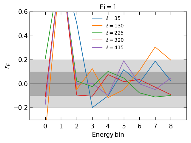


For the sake of validation by summing energy bins together when estimate all bins in Tab. 2, we implement a correlation coefficient to describe the covariance between different energy bins. This Gaussian estimator can be determined by
| (14) |
which the covariance at fixed multipole above in one energy bin is calculating by
| (15) |
The is the coverage percentage of CMB map over full sky map.
With fixed multipole, the illustrates the off-diagonal elements of the covariance between -ray maps and CMB map.
There are four arbitrary energy slices among 9 bins of cross-correlation coefficient in Fig. 4.
For instance, the left-top one is showing the result of first bin with the other 9 bins.
Those peaks are the diagonal of covariance which equal to 1 by definition. Other points are off-diagonal terms.
They show the off-diagonal elements of the covariance matrix in high multipole are mainly below 10% deviation, which means the independence between them.
Despite the correlation are higher at low than other place, which means the different energy bin maps contribute similar way to ISW signal, it allows us to analyze the combining detection by summing them up because of most of them are under 10% deviation.
5 Systematic Tests
To check the robustness of the results, we performed further tests using mock catalogs with no cross correlation with CMB temperature fluctuations, verifying that the computed cross-correlation power spectra are compatible with a null signal.
In each energy bin, we create a Monte Carlo catalog that redistributed the galaxies of the catalog randomly over the sky area and remains the same total flux with the original map. In this case the new catalog contains no intrinsic clustering. Following the procedures above, we could use these random mock catalog to cross-correlate with the Planck map and measure the normalized amplitude parameter. As we expected, the obtained significance is very close to zero, . The clustering feature disappears when using the random mock catalog.
| Samples | Amplitude | SNR | |
|---|---|---|---|
| 1.0 | 1.0 | ||
| 1.7 | 1.6 | ||
| 1.8 | 1.8 | ||
| 1.0 | 0.9 | ||
| 0.4 | 0.4 |
Furthermore, we vary the galactic cut from to in order to test the robustness of our results with the galactic mask. Then we computed the residuals of real Fermi maps using different galactic cut on the mask in all energy bins and measured the cross-correlation power spectra with the Planck map to estimate the significance of ISW detection. In table 3, we list the obtained significance using different galactic cuts on the mask. As we expected, the highest significance comes from the Fermi map with the galactic cut , which is consistent with our previous result (Xia et al., 2011). When we increase the galactic cut area on the mask, the UGRB information will be significantly lost, for example, the area of Fermi map with the cut is only half of that of the map with cut. Therefore, the obtained error bar of the normalized amplitude parameter becomes very large. Consequently, the values of SNR are smaller. When decreasing the galactic cut area, the galactic contamination will be strong and the systematic errors could be larger, which caused the significance lower than before.
6 Conclusions
In this paper, we use the UGRB data in the energy range [0.631, 1000]GeV from the latest Fermi-LAT -ray observation to estimate the cross-correlation power spectra with the Planck CMB map, and investigate its capability on the detection of the well-known ISW effect. Following the procedure of foreground cleaning in Xia et al. (2015); Cuoco et al. (2017); Ackermann et al. (2018), for the first time, we obtain a positive evidence with about significance for the ISW detection from the UGRB information of the Fermi P8 data.
Here we summarize our main conclusions in more detail:
-
•
We report the positive evidence at about confidence level from the cross-correlation power spectra of Fermi -ray maps and Planck CMB map in the energy range [1.202, 2.290] GeV and [17.38, 36.31] GeV. When combining these two energy bins together, we obtain a detection of the ISW effect: (68% C.L.).
-
•
Then we use the single power-law model to normalize the amplitude in each energy bin [equation (12)] and estimate the normalized amplitude parameter from all nine energy bins together. For the first time, we obtain the significance of the ISW effect at about confidence level: . When comparing with the result of Xia et al. (2011), the main improvement comes for the updated Fermi-LAT data.
-
•
Finally, we implement a null hypothesis to test the cross-correlation between CMB and the UGRB of Fermi by randomizing the Fermi maps of nine energy bins, and obtain that these randomized mock Fermi maps contain no intrinsic clustering. This null test confirm the above signal with its near zero significant. The correlation coefficient as an indicator to expose the relation between energy bins, help us to confirm the calculation of combination signal.
-
•
Furthermore, we generate several mask maps with different galactic cut and check the influence of these galactic cut on the obtained significance of ISW effect. Similar with our previous work, we find the galactic cut could give the highest signal to noise ratio.
Acknowledgements
We would like to thank Marco Regis for helpful discussions. This work was supported by the National Science Foundation of China under grants Nos. U1931202, 11633001, and 11690023 and the National Key R&D Program of China No. 2017YFA0402600.
References
- Aghanim et al. (2018) N. Aghanim, et al. (Planck), Planck 2018 results. VI. Cosmological parameters (2018). arXiv:1807.06209.
- Eisenstein et al. (2005) D. J. Eisenstein, et al. (SDSS), Detection of the Baryon Acoustic Peak in the Large-Scale Correlation Function of SDSS Luminous Red Galaxies, Astrophys. J. 633 (2005) 560–574. doi:10.1086/466512. arXiv:astro-ph/0501171.
- Riess et al. (2004) A. G. Riess, et al. (Supernova Search Team), Type Ia supernova discoveries at z ¿ 1 from the Hubble Space Telescope: Evidence for past deceleration and constraints on dark energy evolution, Astrophys. J. 607 (2004) 665–687. doi:10.1086/383612. arXiv:astro-ph/0402512.
- Bacon et al. (2000) D. J. Bacon, A. R. Refregier, R. S. Ellis, Detection of weak gravitational lensing by large-scale structure, Mon. Not. Roy. Astron. Soc. 318 (2000) 625. doi:10.1046/j.1365-8711.2000.03851.x. arXiv:astro-ph/0003008.
- Sachs and Wolfe (1967) R. K. Sachs, A. M. Wolfe, Perturbations of a cosmological model and angular variations of the microwave background, Astrophys. J. 147 (1967) 73–90. doi:10.1007/s10714-007-0448-9, [Gen. Rel. Grav.39,1929(2007)].
- Crittenden and Turok (1996) R. G. Crittenden, N. Turok, Looking for Lambda with the Rees-Sciama effect, Phys. Rev. Lett. 76 (1996) 575. doi:10.1103/PhysRevLett.76.575. arXiv:astro-ph/9510072.
- Boughn et al. (1998) S. P. Boughn, R. G. Crittenden, N. G. Turok, Correlations between the cosmic X-ray and microwave backgrounds: Constraints on a cosmological constant, New Astron. 3 (1998) 275–291. doi:10.1016/S1384-1076(98)00009-8. arXiv:astro-ph/9704043.
- Afshordi et al. (2004) N. Afshordi, Y.-S. Loh, M. A. Strauss, Cross - correlation of the Cosmic Microwave Background with the 2MASS galaxy survey: Signatures of dark energy, hot gas, and point sources, Phys. Rev. D69 (2004) 083524. doi:10.1103/PhysRevD.69.083524. arXiv:astro-ph/0308260.
- Francis and Peacock (2010) C. L. Francis, J. A. Peacock, An estimate of the local ISW signal, and its impact on CMB anomalies, Mon. Not. Roy. Astron. Soc. 406 (2010) 14. doi:10.1111/j.1365-2966.2010.16866.x. arXiv:0909.2495.
- Dupe et al. (2011) F. X. Dupe, A. Rassat, J. L. Starck, M. J. Fadili, Measuring the Integrated Sachs-Wolfe Effect, Astron. Astrophys. 534 (2011) A51. doi:10.1051/0004-6361/201015893. arXiv:1010.2192.
- Nolta et al. (2004) M. R. Nolta, et al. (WMAP), First year Wilkinson Microwave Anisotropy Probe (WMAP) observations: Dark energy induced correlation with radio sources, Astrophys. J. 608 (2004) 10–15. doi:10.1086/386536. arXiv:astro-ph/0305097.
- Scranton et al. (2003) R. Scranton, et al. (SDSS), Physical evidence for dark energy (2003). arXiv:astro-ph/0307335.
- Fosalba et al. (2003) P. Fosalba, E. Gaztanaga, F. Castander, Detection of the ISW and SZ effects from the CMB-galaxy correlation, Astrophys. J. 597 (2003) L89–92. doi:10.1086/379848. arXiv:astro-ph/0307249.
- Granett et al. (2008) B. R. Granett, M. C. Neyrinck, I. Szapudi, An Imprint of Super-Structures on the Microwave Background due to the Integrated Sachs-Wolfe Effect, Astrophys. J. 683 (2008) L99–L102. doi:10.1086/591670. arXiv:0805.3695.
- Chen and Schwarz (2016) S. Chen, D. J. Schwarz, Angular two-point correlation of NVSS galaxies revisited, Astron. Astrophys. 591 (2016) A135. doi:10.1051/0004-6361/201526956. arXiv:1507.02160.
- Goto et al. (2012) T. Goto, I. Szapudi, B. R. Granett, Cross-correlation of WISE Galaxies with the Cosmic Microwave Background, Mon. Not. Roy. Astron. Soc. 422 (2012) L77–L81. doi:10.1111/j.1745-3933.2012.01240.x. arXiv:1202.5306.
- Ferraro et al. (2015) S. Ferraro, B. D. Sherwin, D. N. Spergel, WISE measurement of the integrated Sachs-Wolfe effect, Phys. Rev. D91 (2015) 083533. doi:10.1103/PhysRevD.91.083533. arXiv:1401.1193.
- Boughn et al. (2002) S. P. Boughn, R. G. Crittenden, G. P. Koehrsen, The Large scale structure of the x-ray background and its cosmological implications, Astrophys. J. 580 (2002) 672–684. doi:10.1086/343861. arXiv:astro-ph/0208153.
- Boughn and Crittenden (2004) S. Boughn, R. Crittenden, A Correlation of the cosmic microwave sky with large scale structure, Nature 427 (2004) 45–47. doi:10.1038/nature02139. arXiv:astro-ph/0305001.
- Giannantonio et al. (2008) T. Giannantonio, R. Scranton, R. G. Crittenden, R. C. Nichol, S. P. Boughn, A. D. Myers, G. T. Richards, Combined analysis of the integrated Sachs-Wolfe effect and cosmological implications, Phys. Rev. D77 (2008) 123520. doi:10.1103/PhysRevD.77.123520. arXiv:0801.4380.
- Xia et al. (2011) J.-Q. Xia, A. Cuoco, E. Branchini, M. Fornasa, M. Viel, A cross-correlation study of the Fermi-LAT -ray diffuse extragalactic signal, Mon. Not. Roy. Astron. Soc. 416 (2011) 2247–2264. doi:10.1111/j.1365-2966.2011.19200.x. arXiv:1103.4861.
- Khosravi et al. (2016) S. Khosravi, A. Mollazadeh, S. Baghram, ISW-galaxy cross correlation: a probe of dark energy clustering and distribution of dark matter tracers, JCAP 1609 (2016) 003. doi:10.1088/1475-7516/2016/09/003. arXiv:1510.01720.
- Ade et al. (2014) P. A. R. Ade, et al. (Planck), Planck 2013 results. XIX. The integrated Sachs-Wolfe effect, Astron. Astrophys. 571 (2014) A19. doi:10.1051/0004-6361/201321526. arXiv:1303.5079.
- Ade et al. (2016) P. A. R. Ade, et al. (Planck), Planck 2015 results. XXI. The integrated Sachs-Wolfe effect, Astron. Astrophys. 594 (2016) A21. doi:10.1051/0004-6361/201525831. arXiv:1502.01595.
- Stölzner et al. (2018) B. Stölzner, A. Cuoco, J. Lesgourgues, M. Bilicki, Updated tomographic analysis of the integrated Sachs-Wolfe effect and implications for dark energy, Phys. Rev. D97 (2018) 063506. doi:10.1103/PhysRevD.97.063506. arXiv:1710.03238.
- Camera et al. (2015) S. Camera, M. Fornasa, N. Fornengo, M. Regis, Tomographic-spectral approach for dark matter detection in the cross-correlation between cosmic shear and diffuse -ray emission, JCAP 1506 (2015) 029. doi:10.1088/1475-7516/2015/06/029. arXiv:1411.4651.
- Cuoco et al. (2015) A. Cuoco, J.-Q. Xia, M. Regis, E. Branchini, N. Fornengo, M. Viel, Dark Matter Searches in the Gamma-ray Extragalactic Background via Cross-correlations With Galaxy Catalogs, Astrophys. J. Suppl. 221 (2015) 29. doi:10.1088/0067-0049/221/2/29. arXiv:1506.01030.
- Regis et al. (2015) M. Regis, J.-Q. Xia, A. Cuoco, E. Branchini, N. Fornengo, M. Viel, Particle dark matter searches outside the Local Group, Phys. Rev. Lett. 114 (2015) 241301. doi:10.1103/PhysRevLett.114.241301. arXiv:1503.05922.
- Xia et al. (2015) J.-Q. Xia, A. Cuoco, E. Branchini, M. Viel, Tomography of the Fermi-lat -ray Diffuse Extragalactic Signal via Cross Correlations With Galaxy Catalogs, Astrophys. J. Suppl. 217 (2015) 15. doi:10.1088/0067-0049/217/1/15. arXiv:1503.05918.
- Tröster et al. (2016) T. Tröster, et al., Cross-correlation of weak lensing and gamma rays: implications for the nature of dark matter (2016). doi:10.1093/mnras/stx365. arXiv:1611.03554, [Mon. Not. Roy. Astron. Soc.467,no.3,2706(2017)].
- Cuoco et al. (2017) A. Cuoco, M. Bilicki, J.-Q. Xia, E. Branchini, Tomographic imaging of the Fermi-LAT gamma-ray sky through cross-correlations: A wider and deeper look (2017). doi:10.3847/1538-4365/aa8553. arXiv:1709.01940, [Astrophys. J. Suppl.232,10(2017)].
- Branchini et al. (2017) E. Branchini, S. Camera, A. Cuoco, N. Fornengo, M. Regis, M. Viel, J.-Q. Xia, Cross-correlating the -ray sky with Catalogs of Galaxy Clusters, Astrophys. J. Suppl. 228 (2017) 8. doi:10.3847/1538-4365/228/1/8. arXiv:1612.05788.
- Colavincenzo et al. (2020) M. Colavincenzo, X. Tan, S. Ammazzalorso, S. Camera, M. Regis, J.-Q. Xia, N. Fornengo, Searching for gamma-ray emission from galaxy clusters at low redshift, Mon. Not. Roy. Astron. Soc. 491 (2020) 3225–3244. doi:10.1093/mnras/stz3263. arXiv:1907.05264.
- Tan and Colavincenzo (2019) X. Tan, M. Colavincenzo, Bounds on WIMP dark matter from galaxy clusters at low redshift (2019). arXiv:1907.06905.
- Akrami et al. (2018) Y. Akrami, et al. (Planck), Planck 2018 results. IV. Diffuse component separation (2018). arXiv:1807.06208.
- Kamionkowski (1996) M. Kamionkowski, Matter microwave correlations in an open universe, Phys. Rev. D54 (1996) 4169–4170. doi:10.1103/PhysRevD.54.4169. arXiv:astro-ph/9602150.
- Song et al. (2007) Y.-S. Song, W. Hu, I. Sawicki, The Large Scale Structure of f(R) Gravity, Phys. Rev. D75 (2007) 044004. doi:10.1103/PhysRevD.75.044004. arXiv:astro-ph/0610532.
- Limber (1954) D. N. Limber, The Analysis of Counts of the Extragalactic Nebulae in Terms of a Fluctuating Density Field. II, Astrophys. J. 119 (1954) 655. doi:10.1086/145870.
- Szapudi et al. (2001) I. Szapudi, S. Prunet, S. Colombi, Fast clustering analysis of inhomogeneous megapixel cmb maps (2001). arXiv:astro-ph/0107383.
- Chon et al. (2004) G. Chon, A. Challinor, S. Prunet, E. Hivon, I. Szapudi, Fast estimation of polarization power spectra using correlation functions, Mon. Not. Roy. Astron. Soc. 350 (2004) 914. doi:10.1111/j.1365-2966.2004.07737.x. arXiv:astro-ph/0303414.
- Efstathiou (2004) G. Efstathiou, A Maximum likelihood analysis of the low CMB multipoles from WMAP, Mon. Not. Roy. Astron. Soc. 348 (2004) 885. doi:10.1111/j.1365-2966.2004.07409.x. arXiv:astro-ph/0310207.
- Challinor and Chon (2005) A. Challinor, G. Chon, Error analysis of quadratic power spectrum estimates for CMB polarization: Sampling covariance, Mon. Not. Roy. Astron. Soc. 360 (2005) 509–532. doi:10.1111/j.1365-2966.2005.09076.x. arXiv:astro-ph/0410097.
- Landy and Szalay (1993) S. D. Landy, A. S. Szalay, Bias and variance of angular correlation functions, Astrophys. J. 412 (1993) 64. doi:10.1086/172900.
- Ammazzalorso et al. (2018) S. Ammazzalorso, N. Fornengo, S. Horiuchi, M. Regis, Characterizing the local gamma-ray Universe via angular cross-correlations, Phys. Rev. D98 (2018) 103007. doi:10.1103/PhysRevD.98.103007. arXiv:1808.09225.
- Ackermann et al. (2018) M. Ackermann, et al. (Fermi-LAT), Unresolved Gamma-Ray Sky through its Angular Power Spectrum, Phys. Rev. Lett. 121 (2018) 241101. doi:10.1103/PhysRevLett.121.241101. arXiv:1812.02079.