Search for continuous gravitational waves from ten H.E.S.S. sources
using a hidden Markov model
Abstract
Isolated neutron stars are prime targets for continuouswave (CW) searches by groundbased gravitationalwave interferometers. Results are presented from a CW search targeting ten pulsars. The search uses a semicoherent algorithm, which combines the maximumlikelihood statistic with a hidden Markov model (HMM) to efficiently detect and track quasimonochromatic signals which wander randomly in frequency. The targets, which are associated with TeV sources detected by the High Energy Stereoscopic System (H.E.S.S.), are chosen to test for gravitational radiation from young, energetic pulsars with strong ray emission, and take maximum advantage of the frequency tracking capabilities of HMM compared to other CW search algorithms. The search uses data from the second observing run of the Advanced Laser Interferometer GravitationalWave Observatory (aLIGO). It scans 1Hz subbands around , 4/3, and 2, where denotes the star’s rotation frequency, in order to accommodate a physically plausible frequency mismatch between the electromagnetic and gravitationalwave emission. The 24 subbands searched in this study return 5,256 candidates above the Gaussian threshold with a false alarm probability of 1 per subband per target. Only 12 candidates survive the three data quality vetoes which are applied to separate nonGaussian artifacts from true astrophysical signals. CW searches using the data from subsequent observing runs will clarify the status of the remaining candidates.
I Introduction
The catalogue of gravitational wave (GW) transients [1] observed during the first two observing runs of the Advanced Laser Interferometer GravitationalWave Observatory (aLIGO) and advanced Virgo detectors is a testament to the recent advances in the field of GW astronomy [2, 3]. The signals observed to date primarily come from the coalescence of binary black holes [4, 5, 6] and binary neutron stars [7, 8]. An isolated neutron star whose mass is distributed asymmetrically about its rotation axis is also a promising source of persistent, quasimonochromatic continuous gravitational waves (CW) [9, 10]. Emission from such sources is predicted to be at multiples of the star’s spin frequency [11]. For example, a mass quadrupole caused by a thermoelastic or magnetic mountain emits a CW signal at and [12, 13], rmodes emit at roughly /3 [14] and a current quadrupole produced by nonaxisymmetric circulation of neutron superfluid pinned to the crust emits a signal at [15].
Extracting a CW signal from noisy detector data often involves matched filtering against a bank of templates. Managing the size of this template bank and thus the computational cost of the search is an important part of designing a practical search [16, 17]. For a coherent search over a total observation time , the required number of templates grow as , whereas the sensitivity increases as [18]. The value of the exponent is determined by the number of unknown parameters. For example, one has for an allsky search, which typically involves searching over sky position, frequency, and frequency derivatives [18].
In a search directed at a particular object, such as the one described here, typically has a smaller value as the sky position, and in many cases, some frequency derivatives are known. Nevertheless the computational challenge is acute, and it is common to use a semicoherent approach, which involves dividing the search into short blocks of length , coherently searching for signals in each block, and then incoherently combining these blocks to cover the entire search space. The sensitivity of a semicoherent search than scales as [18]. Although this makes it less sensitive than coherent matched filtering, it allows more data to be used, which in turn improves the sensitivity of the search while allowing it to remain computationally tractable [18].
Phase templates for CW signals from isolated pulsars are often expressed as Taylor expansions about some reference time of form (e.g., see Eq. (18) in Ref. [19])
| (1) |
where is the phase at the reference time, is the time derivative of evaluated at and is the highestorder time derivative included in the search. One therefore has , which grows rapidly with [20].
The challenge increases dramatically when the phase of the signal wanders stochastically on timescales of days to weeks. Radio and Xray timing of isolated pulsars show “spinwandering” to be a widespread phenomenon, often going by the name timing noise [21, 22, 23]. It is attributed to various mechanisms including changes in the star’s magnetosphere [24], spin microjumps [25], superfluid dynamics in the stellar interior [26, 27] and fluctuations in the spindown torque [28, 29]. It is especially pronounced in young pulsars with characteristic ages kyr [30, 21], among which include three targets in this paper. While spinwandering could, in principal, be modelled with higherorder derivatives, the number of derivatives required would make impractically large and thus make the search computationally infeasible.
In this paper, we use a hidden Markov model (HMM) solved by the classic Viterbi algorithm to search for CW signals from isolated neutron stars. This scheme combines an existing, efficient and thoroughly tested maximum likelihood detection statistic called the statistic [19] with a HMM. Loosely speaking, the statistic coherently searches for a constantfrequency signal within a block of data, and the HMM tracks the stochastic wandering of the signal frequency from one block to the next [31]. The method shares some common elements with other semicoherent methods such as StackSlide [20, 32] and facilitates the use of data from the entire second observing (O2) run while remaining computationally manageable. Finally, it can accommodate the situation where the gravitationalwaveemitting quadrupole is not phase locked to the stellar crust, even when the ephemeris is accurately measured via electromagnetic observation [33].
To sharpen the astrophysical focus of the search, we select 10 pulsars whose pulsations and/or pulsar wind nebulae have been observed by very highenergy (VHE) ray surveys such as the High Energy Stereoscopic System (H.E.S.S.) and the Very Energetic Radiation Imaging Telescope Array System (VERITAS). Previous CW searches have searched for signals from eight of these targets [34, 35, 33, 36, 37, 38, 39, 40, 41, 42, 43]. Leptonic models are often used to completely describe the TeV rays originating from these sources [44, 45, 46]. The ray emission is unlikely to be tied directly to a gravitationalwaveemitting mass or current quadrupole, as it comes from lowdensity plasma accelerated in magnetosphere vacuum gaps [47, 48]. However, it is entirely possible that ray emission is a reliable cosignature of gravitational radiation, because it is tied to young pulsars, whose mass and current quadrupoles at birth have had relatively little time to relax via slow dissipative processes [49, 50, 51]. Moreover such objects are surrounded by active magnetospheric and particle production processes, which may react back on the star. For example, the heating of polar caps by downwardmoving particles bombarding the stellar surface can induce nonaxisymmetric variations in the stellar mass density and thus yield a gravitationalwaveemitting mass quadrupole [52, 53, 54, 55].
In anticipation of a future detection, it is crucial to note that the TeV spectrum provides a comprehensive picture of the electron population around the pulsar [56]. We can therefore obtain better estimates for the age and magnetic field strength around the progenitors, while multiwavelength observations can yield accurate estimates of the distance to the source. Therefore, the sources in this paper offer unusually rich opportunities to do highimpact astrophysics in the event of a detection. Likewise, in the absence of a detection, the accurate age, distance, and magnetisation measurements can be converted into accurate GW spindown upper limits [9, 57, 41] to be interpreted in the light of the upper limits from the GW search.
This paper is organised as follows. We outline the targets selected for this study and briefly review their GeV and TeV properties in Section II. In Section III, we review the results from previous CW searches targeting the selected pulsars. Section IV explains the search algorithm which includes a review of the signal model, the detection statistic known as the statistic and the HMM formulation. In Section V, we define the search parameter space for each pulsar as well as the detection threshold and data quality vetoes. The results are presented in Section VI. We conclude with a brief statement on the astrophysical implications in Section VII.
II Targets
The targets for this search are selected from the publicly available TeV catalogue 111http://tevcat2.uchicago.edu/. We restrict the analysis to TeVemitting pulsars, sources firmly associated with isolated neutron stars and located within the galactic disk (i.e., up to a distance of 7kpc). With these restrictions in place, the catalogue includes two rayemitting pulsars and eight H.E.S.S. sources firmly identified as pulsar wind nebulae (PWNe) powered by known pulsars. Table 1 gives the astrophysical parameters for the ten targets. Note that a small discrepancy exists between the position of the H.E.S.S. sources and their associated pulsar due to the pulsar being offset from the centre of the TeV emission region, possibly due to its proper motion, asymmetric crushing of the PWN by the surrounding supernova remnant or by asymmetric pulsar outflow [46, 59]. Below, we briefly discuss the GeV and TeV properties of the H.E.S.S. targets.
| HESS name | Pulsar name | RA | DEC | Age | Distance | Spin frequency |
|---|---|---|---|---|---|---|
| J2000] | [J2000] | [kyrs] | Min/Max [kpc] | [Hz] | ||
| - | J05342200 | 1.26 | 1.5/2.5 | 29.946923(1) | ||
| - | J08354510 | 11.3 | 0.26/0.30 | 11.1946499395(5) | ||
| J1018589 B | J10165857 | 21 | 3.16/8.01 | 9.31216108951(13) | ||
| J1356645 | J13576429 | 7.31 | 2.83/3.88 | 6.0201677725(5) | ||
| J1420607 | J14206048 | 13 | 5.63 | 14.667084337(5) | ||
| J1514591 | J15135908 | 1.57 | 3.6/5.7 | 6.59709182778(19) | ||
| J1718385 | J17183825 | 89.5 | 3.49/3.60 | 13.39227352093(7) | ||
| J1825137 | J18261334 | 21.4 | 3.61/3.93 | 9.85349875132(2) | ||
| J1831098 | J18310952 | 128 | 3.68/4.05 | 14.8661645038(3) | ||
| J1849000 | J18490001 | 43.1 | 7 | 25.961252072(9) |
PSR J05342200 (Crab pulsar): Fermi Large Area Telescope (FermiLAT) observations of the rays emitted by the Crab pulsar reveal a light curve with two main peaks, labelled P1 and P2, both of which are extremely stable in position across the ray energy band (See Fig. 1 of Ref. [64]). The first ray pulse leads the radio pulses by 281s [64]. This combined with the measurement of photons up to 20GeV constraints the production site of nonthermal emission in the pulsar magnetosphere [64]. In addition, observations taken by VERITAS between 20072011 reveal ray pulses at energies 100GeV [65] which are narrower than those recorded by FermiLAT at 100MeV. Combined analysis of FermiLAT and VERITAS data yields important information about the shape and location of the particle acceleration site and TeV emission mechanism [65].
PSR J08354510 (Vela pulsar): FermiLAT observations of this pulsar reveal two narrow and widely separated pulses (labelled P1 and P2) typically observed in high energy pulsars [66]. A complex bridge emission (labelled P3) is also observed between the two main peaks (See Fig. 2 of Ref. [67]). H.E.S.S. IICT5 observations from 2013 to 2015 confirm the characteristics previously known from FermiLAT studies and reveal a change in the P2 pulse morphology as well as the onset of a new component near P2 at higher energies [68]. FermiLAT and H.E.S.S. measurements of the phaseaveraged spectrum also contains important information about the location and origin of TeV emission [67].
HESS J1018589B: This is one of two regions of TeV ray emission around the supernova remnant G284.31.8. The TeV emission has a radius of and is likely to be associated with a pulsar wind nebula powered by PSR J10165857 [69].
HESS J1356-645: The morphology of this source in radio and Xrays, combined with its spectral energy distribution in TeV, as measured by FermiLAT in 2013, leads to its classification as a clearly identified PWN [70]. The emission is most likely associated with the young and energetic pulsar PSR J13576429, which is located at a distance of 5pc from the center of the TeV emission [71].
HESS J1420607 (Kookaburra PWN): This is one of the two TeV sources in a complex of compact and extended radio and Xray sources, called Kookaburra. It is centered north of a young and energetic pulsar PSR J14206048, believed to be one of the sources powering the complex [72]. Pulsed ray and extended Xray emissions from the source provide evidence for its PWN nature [73].
HESS J1514591 (MSH 1552):
This composite supernova remnant contains a bright Xray PWN powered by PSR J15135908 which is surrounded by a shell that dominates the emission in the radio band. Correlation between the H.E.S.S. and Xray data and pulsar jets in the Xray domain lead to its classification as a clearly identified PWN [74]. The TeV morphology also suggests asymmetric expansion of the supernova remnant, displacing the PWN in the direction away from the high photon density region [75].
HESS J1718385: Observation of this H.E.S.S. source by the space based Xray MultiMirror Mission (XMMNewton) reveals a hard Xray source at the position of PSR J17183825. Diffuse emission in the vicinity of the pulsar suggests the existence of a synchrotron nebula and strengthens its association with the pulsar. However, the relationship between the Xray and ray emission is not straight forward. The overall asymmetry of the nebula with respect to the pulsar is consistent with the idea of supernova remnant expanding into a nonuniform environment [76].
HESS J1825-137: TeV emissions from the PWN extend out to 1.5∘ from the pulsar’s location, which makes it one the most luminous and potentially the largest of all firmly identified PWNs in the Milky Way [77]. The XMMNewton’s observation of the region, including the pulsar, reveals an elongated nonthermalemitting nebula with the pulsar located on the northern border and a tail towards the peak of the H.E.S.S. source. This is also consistent with TeV rays originating from the inverse Compton mechanism within the PWN powered by PSR J18261256 [78].
HESS J1831098: Detected by the H.E.S.S. survey in 2011, this source is proposed to be a member of a new class of TeV emitters known as extended TeV halos [79]. A 67ms pulsar, PSR J18310952, lies at a small angular offset of 0.05∘ from the bestfit position of the H.E.S.S. source. A conversion efficiency from spindown power to 120 TeV rays of would be required to power this H.E.S.S. source, a value typically inferred for other TeV/PWN systems. This combined with the lack of other plausible counterparts in multiwavelength searches provides evidence for a PWN as the most favorable scenario [80].
HESS J1849-000: This extended TeV source is coincident with a hard Xray source IGR J184900000 [81]. Followup observations of the source by XMMNewton and Rossi Xray Timing Explorer confirm HESS J1849000 as a PWN powered by a young and energetic pulsar, PSR J18490001 [63]. This study also provides clear evidence of a PWN that is asymmetric in Xrays [82].
III Previous pulsar searches
Numerous CW searches have previously looked for signals from eight of the targets chosen for this study. In particular, PSR J05342200 (Crab) has been extensively studied using data from the LIGO science runs (S) 25 [34, 35, 33, 36] and Virgo science run (VSR) 4 [33]. Most of these searches exploited a Bayesian method, except Refs. [36] and [33] which used Markov Chain Monte Carlo (MCMC) and 5nvector techniques, respectively. Although none of these searches found strong evidence of a CW signal from the Crab pulsar, they improved the upper limits (ULs) on the GW strain amplitude from to over a period of five years.
Data from VSR2 [37] and VSR4 [39] was used to search for a CW signal from PSR J08354510 (Vela). These searches were carried out using three largely independent methods; Bayesian and -statistic methods in Ref. [37] and a 5n-vector method in Ref. [39]. No CW signal was detected and ULs were set on the GW strain amplitude. In 2014, Aasi et al. combined observations from S6, VSR2 and VSR4 to look for CW signals from 179 pulsars [38], four of which are included in this HMM search. For seven highvalue targets, the search was performed using three largely independent methods; Bayesian, -statistic, and 5n-vector methods. Only the Bayesian method was applied to the remaining 172 pulsars. The search found no credible evidence for GW emission from any pulsar and produced ULs on the emission amplitude.
In early 2017, Abbott et al. [41] repeated a similar analysis for 200 pulsars, five of which are considered here, using the data from aLIGO’s first observing run (O1). For 11 highvalue targets, the search was performed using the Bayesian, -statistic, and 5n-vector methods. Only the Bayesian method was used for the remaining 189 pulsars. No detections were reported, and ULs were set on the GW strain amplitude and ellipticity of each target.
Following the second observing run (O2), Abbott et al. [42] performed a CW search for 33 pulsars using the 5n-vector pipeline. These included three of the targets chosen for this study. The narrowband search found no evidence for a GW signal from any of the targets, but significantly improved on ULs for pulsars with rotation frequency 30Hz. Later that year, Abbott et al. [43] combined data from O1 and O2 to search for CW signals from 222 pulsars at and . As in Ref. [40], they used Bayesian, -statistic and 5n-vector methods for 34 highvalue targets and only the Bayesian method for the remaining 188 pulsars. Although the search found no strong evidence for GW emission from any pulsar, it did allow for updated ULs on the GW amplitude, mass quadrupole moment and ellipticity for 167 pulsars, and first such limits for 55 others.
We summarise the ULs set by the aforementioned studies for targets relevant to this search in Table 2. Although these targets have been studied in the past, the HMM enables the examination of a much more inclusive set of spinwandering templates than the Taylorexpanded phase model assumed in the above references. Young pulsars with TeV ray emission, such as the ones considered here, exhibit rapid spinwandering. Hence they derive maximum benefit from being searched again with a HMM.
| Name J2000 | Observing run | Search method(s) | [] | Ref |
| J05342200 | O1O2 | Bayesian, statistic, 5nvector | 0.19(0.15), 0.22(0.13), 0.29(0.29) | [43] |
| O2 | 5nvector | 1.64[BG], 1.31 [AG] | [42] | |
| O1 | Bayesian, statistic, 5nvector | 0.67(0.61), 0.42 (0.24), 0.52 (0.50) | [41] | |
| SR6, VSR2 VSR4 | Bayesian, statistic, 5nvector | 1.6(1.4), 2.3 (1.8), 1.8(1.6) | [38] | |
| VSR4 | 5nvector | 7.0 | [39] | |
| S5 | MCMC | 2.4 | [36] | |
| S5 [1st 9 months] | Bayesian/statistic | 4.9/3.9 | [33] | |
| SR3SR4 | Bayesian | 30.9 | [35] | |
| SR2 | Bayesian | 410 | [34] | |
| J0835-4510 | O1O2 | Bayesian, statistic, 5nvector | 1.4(1.2), 2.6(2.0), 2.3(2.4) | [43] |
| O2 | 5nvector | 8.82 | [42] | |
| O1 | Bayesian, Fstatistic, 5nvector | 3.2(2.8), 3.8 (3.3), 2.9 (2.9) | [41] | |
| SR6, VSR2 VSR4 | Bayesian, statistic, 5nvector | 11(10), 4.2(9.0), 11(11) | [38] | |
| VSR4 | 5nvector | 32 | [39] | |
| VSR2 | Bayesian, statistic,5nvector | 21(1), 19(1), 22(1) | [37] | |
| J1016-5857 | O1 | Bayesian | 14 | [41] |
| J1420-6048 | O1O2 | Bayesian, 5nvector | 0.41, 0.76 | [43] |
| O2 | 5nvector | 2.75 | [42] | |
| J1718-3825 | O1O2 | Bayesian, 5nvector | 0.87, 0.65 | [43] |
| O1 | Bayesian | 1.7 | [41] | |
| SR6, VSR2 VSR4 | Bayesian | 0.80 | [38] | |
| J1826-1334 | O1 | Bayesian | 12 | [41] |
| J1831-0952 | O1O2 | Bayesian, 5nvector | 0.69, 0.43 | [43] |
| SR6, VSR2 VSR4 | Bayesian | 0.65 | [38] | |
| J1849-0001 | O1O2 | Bayesian, statistic, 5nvector | 0.19, 0.28, 0.20 | [43] |
IV Search Algorithm
In this paper, we subdivide the total observation time into blocks of duration , during which the signal frequency is assumed to remain constant to a good approximation. Within each block, we search for a signal predicted to be emitted by a biaxial rotor by coherently combining the detector data. This data is available in the form of short Fourier transforms (SFTs), each with length = 30min. In Sections IV.1 and IV.2, we review the signal model and the maximum likelihood detection statistic called the statistic, as defined in Ref. [19]. Finally, we incoherently combine the output of each block and recover the optimal frequency path through the data using a HMM. We briefly review the HMM framework in Section IV.3.
IV.1 Signal model
In the absence of noise, we model the GW strain from a pulsar as
| (2) |
where denote the amplitudes associated with four linearly independent components, as defined in Eqs. (28)(31) of Ref. [19]. They depend on parameters such as the characteristic strain (), sky location (RA, DEC), source inclination with respect to the line of sight (), initial phase () and wave polarisation. Here, represents four linearly independent components
| (3) | ||||
| (4) | ||||
| (5) | ||||
| (6) |
where and are the antennapattern functions as defined in Eqs. (12) and (13) of Ref. [19]. The signal phase, , as measured by a detector on Earth, includes contributions from three terms [83],
| (7) |
where represents the time shift produced by the diurnal and annual motion of the detector relative to the solar system barycentre. The term represents the phase shift which results from the intrinsic evolution of the source in its rest frame through the frequency derivatives [ with ].
The frequency evolution of a CW signal has a secular and a stochastic term. The (slow) secular spindown of the pulsar can be easily modelled by specifying the frequency derivatives measured via electromagnetic observations. However, the stochastic term cannot be easily measured, and it is computationally infeasible to conduct an exhaustive search over physicallyplausible stochastic paths. Instead, we use a HMM, as outlined in Section IV.3, to handle the stochastic evolution of the signal phase and the Viterbi algorithm to efficiently backtrack the optimal pathway in frequency. In other words, in this paper, we set according to the spindown rate () reported in a pulsar catalogue and set higher derivatives to zero within each coherent block. We then let the HMM (instead of the Taylor expansion) do the work of tracking , as it evolves from one block to the next.
IV.2 -statistic
Following Ref. [19], we use the maximum likelihood statistic to extract a CW signal buried in detector noise. The statistic involves maximising the likelihood function () with respect to the amplitudes . The values of the parameters which maximise are known as the maximum likelihood estimators. Below, we briefly review how the statistic is defined.
The timedependent output of a single detector can be assumed to take the following form [19]:
| (8) |
where represents stationary, additive noise and is the GW signal as defined in Eq. 2. We can then define a normalised loglikelihood function of form [19]
| (9) |
where the inner product is given by
| (10) |
By maximising with respect to the four amplitudes () over the observation period (), we find the optimal set of signal parameters. These parameters, also known as the maximum likelihood (ML) estimators, are then used to define a frequency-domain detection statistic called the statistic of form
| (11) |
with , , and . A full derivation of Eq. (11) can be found in Sec III.A of Ref. [19].
We claim a detection if the functional exceed a predefined threshold, which is calculated to give a desired false alarm probability. Once above threshold, the magnitude of indicates the probability of detection [19]. In the case of white, Gaussian noise with no signal, the probability density function (PDF) for the statistic takes the form of a centralised distribution with four degrees of freedom, . When a signal is present, the PDF has a noncentral distribution with four degrees of freedom, . The noncentrality parameter is
| (12) |
where the constant depends on the number of detectors, orientation of the source and the sky location, is the characteristic strain of the GW signal, and represents the onesided noise spectral density of the detector.
IV.3 HMM framework
A HMM offers a powerful method for detecting and tracking the wandering frequency of a pulsar [31]. This is done by modelling the signal frequency probabilistically as a Markov chain of transitions between unobservable (hidden) states and using the statistic as a detection statistic to relate the observed data to the hidden states. HMM tracking plays a critical role in various industrial applications including computational biology [84], radar target detection systems [85] and biometric recognition [86]. It estimates accurately when the signaltonoise ratio is low but the sample size is large, a situation commonly encountered in CW searches [31]. HMMs have been used to search for CW signals from lowmass Xray binary systems [83, 87, 88], supernova remnants [89] and the postmerger remnant of GW170817 [90].
As in Ref. [83], we model the spin parameter of a CW signal as a hidden Markov process where the hidden (unobservable) state variable transitions between values in a set {} at discrete times {}. Meanwhile, the observable state variable transitions between values from the set {}. Under the Markov assumption, the hidden state at time only depends on the state at time . This is described by the transition probability matrix
| (13) |
The likelihood that the hidden state gives rise to the observation is described by the emission probability matrix
| (14) |
Finally, the model is completed by specifying the probability of the system occupying each hidden state initially, which is described by the prior vector
| (15) |
For a Markov process, the probability that a hidden path } gives rise to the observed sequence can be obtained using the following expression [91]
| (16) |
The path which maximises is known as the most probable path and is defined as
| (17) |
The Viterbi algorithm, as outlined in Refs [91, 23] provides a recursive, computationally efficient route to computing from Eqs. (13) to (17). It relies on the Principle of Optimality, which states that all subpaths of an optimal path are themselves optimal [92]. To speed up the computation process, we evaluate , whereby Eq. (16) becomes a sum of loglikelihoods.
Previous HMM searches [88, 83] have modelled timing noise as an unbiased random walk, in which the frequency of the signal () moves by at most one bin up or down during a timescale . This is represented by the following transition matrix
| (18) |
An unbiased random walk is not appropriate in this paper because, for all targets considered here, the evolution of is dominated by the secular spindown of the pulsar rather than its timing noise [Refer to Section V.2, Table 3]. Consequently, the secular spindown sets and moves down by one bin in each segment. Since the stochastic spinwandering timescales are typically longer than the secular timescales, one could argue that an appropriate transition matrix would be the trivial matrix:
| (19) |
However, the drift timescales given in Table 3 are conservative estimates, they are only estimates and significant modelling uncertainties remain, particularly because the precise mechanism of GW emission is not yet established. With such a precise prescription as in Eq. (19), any spinwandering leads to a substantial loss of sensitivity [22]. Therefore, it is appropriate to model the system as a biased random walk, with the bias in this case accounting for the secular spindown. A looser prescription also ensures that the HMM can continue to track the signal even if is mis-measured or if the emission frequency shifts randomly (e.g. due to internal stellar processes [27]) with respect to . The resulting transition matrix is
| (20) |
with all other terms being zero. For simplicity, we choose equal weighting for the three allowed transitions, which does not have a significant effect on sensitivity of such searches [89].
The emission probability takes the following form [91, 89]
| (21) |
where the is computed for each segment of length at a frequency resolution of . Section V.2 outlines the criteria used for setting . We choose a uniform prior over the subband expected to contain the GW signal (see Section V.1):
| (22) |
where is the total number of frequency bins.
V Searching O2
We use publicly available data from the O2 run of the aLIGO detectors, specifically the GWOSC4KHzR1STRAIN channel, to search for CW signals from the pulsars listed in Table 1 [93]. This observing run took place between 30112016 and 25082017. The advanced Virgo detector was also operating for the last month of O2. However, we do not use the data from this detector due to its relatively short observation period and lower sensitivity [93]. During O2, there was a break in the operation of both detectors from 22122016 23:00:00 UTC to 04012017 16:00:00 UTC. In addition, a commissioning break took place at the Livingston detector between 08052017 and 26052017, while at the Hanford detector it lasted from 08052017 to 08062017 [93]. In order to perform a joint search between the two aLIGO detectors, we choose a common period from 04012017 to 25082017, with a total 234 days.
In Sections V.1 and V.2, we outline the procedure for setting the search parameters, namely the frequency range and coherence timescale. In Section V.3, we briefly discuss whether pulsar glitches have any affect on this search. Section V.4 outlines the procedure for setting the detection threshold. Finally, we describe the vetoes used to distinguish a real signal from a nonGaussian noise feature in Section V.5.
V.1 Frequency range
All of the targets chosen for this study are observed to pulse electromagnetically, meaning their spin frequency is known to a precision of at least one part in a million. We use v1.63 of the Australian Telescope National Facility (ATNF) pulsar catalogue [60] to obtain an accurate ephemeris for each pulsar. The search is carried out at simple multiples of the star’s spin frequency (, and ) to account for the different emission mechanisms listed in Section I [15]. We search a 1Hz subband around each multiple to accommodate stochastic spinwandering, secular spindown and the possibility that the signal is displaced systematically from the relevant multiple of , i.e., because the Xrayemitting crust and GWemitting quadrupole are not exactly locked together [94, 95]. The HMM’s speed enables us make the subbands generously wide, viz. 1Hz, and track a larger set of spectral displacements and spinwandering histories than typical coherent searches based on a Taylor series phase model [43, 41, 33, 38, 37]. We do not search in subbands where the expected signal frequency falls below 10Hz as the strain data is not calibrated below this frequency. This is primarily because the detector noise rises rapidly below 10Hz and is significantly larger than any plausible GW strain signal. Additionally, the GW open data is aggressively highpassfiltered at 8Hz to avoid signal processing issues and thus does not accurately represent either the signal or noise at low frequencies [96, 93].
V.2 Coherence timescale
The coherence timescale, , is an important parameter as it sets the frequency resolution () of the search. It is chosen such that the signal frequency falls in one frequency bin during a single coherent step. For each pulsar, we weigh the drift timescale expected due to the secular spindown () against the stochastic spinwandering timescale (). We then use the shorter of the two timescales to define for this search.
Overestimating the drift timescale means that, in general, the CW signal wanders by more than one search frequency bin (i.e., ) over a single coherent step of length . This presents a difficulty for the HMM tracker, which can only “keep up” with signals that wander down by zero, one or two bins per coherent step, as defined by the transition matrix in Eq. 20. Once the HMM loses track, the phase mismatch between the signal and model increases monotonically, and the signal-to-noise ratio (SNR) decreases, until it falls below the detection threshold [97].
In contrast, underestimating does not affect the tracking ability of the HMM; the drift condition given by Eq. 24 is still satisfied, and the HMM can easily track the signal. However, shorter coherence timescales increase the total number of segments () which are combined incoherently, reducing the sensitivity of the search, which scales as [18]. For this reason, it is arguably safer to underestimate rather than overestimate .
V.2.1 Spindown timescale
The spindown rate of a pulsar is governed by the rate at which rotational energy is extracted by magnetic dipole and gravitational quadrupole radiation [98, 99]. The spindown drift timescale () is chosen to satisfy the following relation, satisfying mismatch 0.2 [89]:
| (23) |
Here, represents the frequency resolution of the search. We also require the change in the signal frequency due to the secular spindown over [] to satisfy
| (24) |
for [89]. Even though the signal frequency may not be locked to the star’s spin frequency [94, 95], we can assume that to a good approximation. Combining relation 23 with 24, we arrive at the following equality
| (25) |
Hence, one obtains , which depends solely on the spindown rate of the pulsar (). We obtain the most conservative estimate for by using , where denotes the maximum allowed value of from electromagnetic observations. The spindown drift timescales for the ten targets are presented in column 3 of Table 3.
V.2.2 Stochastic spinwandering timescale
Pulsar timing measurements reveal stochastic spinwandering as a widespread phenomenon which manifests itself as timing noise [21, 22], autocorrelated on the order of days to weeks [23]. The timing noise in pulsars can be characterised as a random walk in some combination of rotation phase, frequency and spindown rate. These idealised cases are commonly referred to as phase noise, frequency noise and spindown noise [100, 101]. The stochastic spinwandering timescale () can be estimated in terms of two parameters defined below, and , which characterise the power spectral density (PSD) of the timing noise phase residuals [102]. One finds
| (26) |
refer to Appendix B for a full derivation. In equation 26, is the exponent of powerlaw PSD of phase residuals, [101, 102]. Also in Eq. 26, we have the parameter which is defined as follows
| (27) |
where is the rms phase residual accumulated over timegap . Depending on which random process best describes the observed timing noise, can be 2, 4 or 6 for phase noise, frequency noise or spindown noise, respectively. The spectral index has only been measured for a handful of the selected targets, namely the Crab pulsar ( = 4) [103], Vela pulsar ( 6) [101] and PSR J15135908 ( 6) [102]. For the remaining targets, we experiment with all three scenario (i.e., ) and quote the most conservative timescale (i.e., shortest ) in Table 3, obtained using .
Conservatives estimates for the two drift timescales indicate that on average. We pick . Tables 615 in Appendix A summarise the search parameters for each target.
| Pulsar name | Spindown rate | |||
|---|---|---|---|---|
| J2000 | [ Hzs-1] | [days] | [Cycles] | [yrs] |
| J05342200 | 377.535(2) | 0.41 | 0.003 | 1.902 |
| J08354510 | 15.666(6) | 2.06 | 4.9 | 0.609 |
| J10165857 | 7.00965(5) | 3.08 | 0.0401 | 2.87 |
| J13576429 | 13.05395(5) | 2.25 | 0.0217 | 1.51 |
| J14206048 | 17.8912(7) | 1.94 | 1.02 | 0.57 |
| J15135908 | 66.5310558(2.7) | 1.00 | 1.97 | 4.52 |
| J17183825 | 2.371346(1.1) | 5.31 | 0.361 | 1.73 |
| J18261334 | 7.3062994(9) | 3.02 | 22.35 | 1.79 |
| J18310952 | 1.839595(5) | 6.04 | 0.0297 | 13.04 |
| J18490001 | 9.59(4) | 2.63 | 0.0136 | 1.52 |
V.3 Glitches
Glitches are another form of timing irregularity commonly observed in a subset of the isolated pulsar population [62]. They show up as abrupt changes in , often followed by a relaxation. Glitches offer an opportunity to probe the interior of a neutron star and the properties of matter at supernuclear densities [104, 105].
The Crab pulsar underwent a small glitch on 27032017 222http://www.jb.man.ac.uk/pulsar/glitches.html. This event changed the star’s spin frequency by Hz which is significantly smaller than Hz. The Vela pulsar also experienced a glitch on 12122016, at the start of O2 [107, 108], with Hz. This is conveniently outside the chosen observation period and does not affect our analysis. None of the other pulsars are reported to have glitches in the chosen observation period.
V.4 Threshold
As outlined in Section IV, we apply the statistic to the O2 dataset to calculate the probability of a signal being detected for a given set of parameters. We then use the Viterbi algorithm to find a set of optimal paths through the frequency space. Each optimal Viterbi path ends in one of the final states () and has an associated loglikelihood as defined in Eq. 16. A path is classified as a detection candidate if its exceeds a predetermined threshold .
We aim to find such that the search has a false alarm probability P per subband, per target. To do this, we generate 100 Gaussian noiseonly realisations for each subband using the lalappsMakefakedatav4 tool in the LIGO Scientific Collaboration Algorithm Library (LAL) [109]. Each realisation is searched using the procedure outlined in Section IV, and is chosen to yield at-most one (false) detection [88]. The thresholds obtained using the above procedure are listed in the third column of Table 4.
V.5 Vetoes
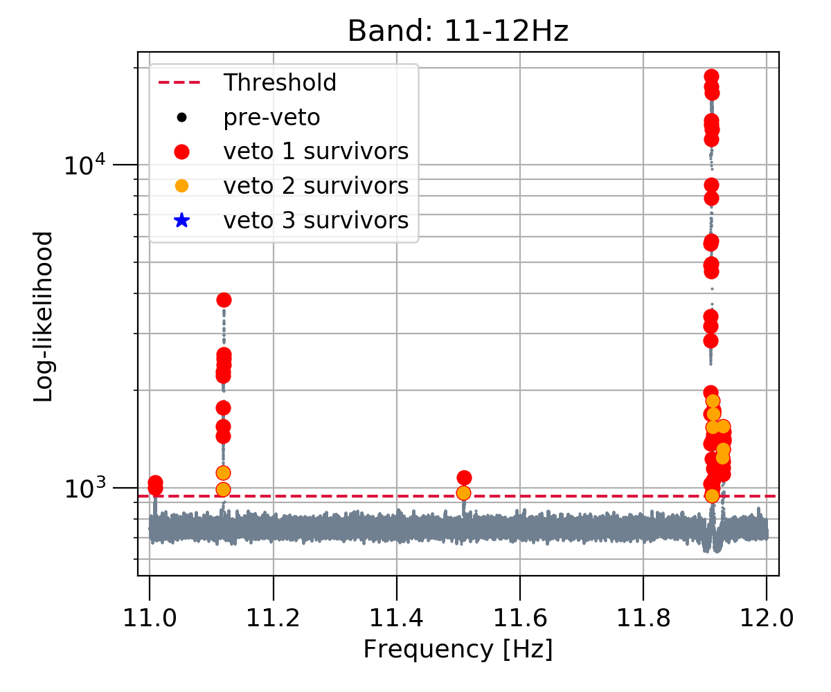
Some of the signal templates produce candidates with . The number of candidates may exceed the number expected from Pfa because of nonGaussian features in the real aLIGO detector noise. Here we lay out three veto criteria used to discard candidates as nonastrophysical sources. These are adapted from the vetoes previously used in published HMM searches [83, 87, 88].
-
1.
Known lines veto: Numerous persistent instrumental lines are identified during the aLIGO detector characterisation process [110]. These lines are produced by a number of sources, including resonant modes of the suspension system, external environmental causes and interference from equipment around the detector [87]. If the Viterbi path of a candidate crosses a known noise line over the duration of the observing run, it can be safely vetoed as a known instrumental line.
-
2.
Single interferometer (IFO) veto: A strong noise artifact which is only present in one of the detectors can produce candidates above threshold in the twindetector search. To veto such artifacts, we analyse the data from the Hanford and Livingston detectors separately and compare the loglikelihood in each case (i.e., and ) with the loglikelihood from the twindetector search (). If in either interferometer (but not both) exceeds , the candidate can be safely vetoed as an instrumental artifact. Otherwise we keep the candidate for further analysis.
-
3.
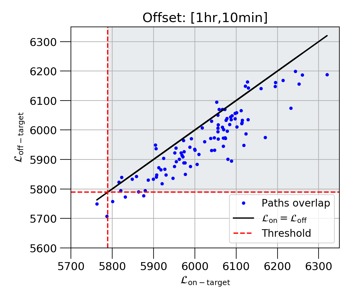
Offtarget veto: This veto was first introduced in Ref. [88] and extensively studied in Refs. [111, 112, 113]. It involves analysing the detector data in an offtarget sky position. For this study, we offset the search from the pulsar’s sky location by in right ascension and in declination, while keeping all other parameters of the search constant. If the offtarget search returns 0.9, where denotes the loglikelihood from the dual interferometer, ontarget search, we veto the candidate as an instrumental artifact. This veto criteria is based on the outcome of the injection studies presented in Appendix C.
Previous HMM searches have used an additional veto, known as the veto, whereby the data is split in two halves and each half is analysed separately [83, 87]. A true astrophysical signal should be present in both segments unless it is a transient source like an rmode which happens, by luck, to be off for half of the observation [114]. These searches used Viterbi score as a detection statistic, which is defined as the number of standard deviations the loglikelihood of the optimal path exceeds the mean loglikelihood of all alternative pathways. Due to the normalisation step, which is inherent to the score calculation, the distribution of final is (approximately) the same for typical observation lengths. This implies that the detection statistic is independent of . However, since the distribution of unnormalised varies with , separate thresholds will need to be established for the two data segments in order to adapt the veto to this search. For this reason, we do not use here.
VI Results
All of the targets listed in Table 1 return candidates with . This is not surprising as the detector noise is not Gaussian. We apply the three data quality vetoes outlined in Section V.5 to each candidate to separate a real signal from a nonGaussian noise artifact. The results are summarised in Table 4 while Figs. 1322 in Appendix D show against the terminating frequency of the Viterbi paths for each subband of each target. The search returns 5,256 candidates across 24 subbands, only 12 of which survive the three data quality vetoes.
| Pulsar name | Subband | Candidates | Candidates | |
| J2000] | [Hz] | (preveto) | (postveto) | |
| J05342200 | 29.530.5 | 4090 | 11 | 1 |
| 39.540.5 | 4775 | 9 | 0 | |
| 59.560.5 | 5789 | 12 | 0 | |
| J08354510 | 1112 | 943 | 64 | 0 |
| 14.515.5 | 1069 | 196 | 0 | |
| 2223 | 1290 | 54 | 0 | |
| J10165857 | 1213 | 756 | 29 | 0 |
| 1819 | 896 | 10 | 0 | |
| J13576429 | 11.512.5 | 1187 | 44 | 0 |
| J14206048 | 1415 | 1006 | 58 | 1 |
| 1920 | 1146 | 46 | 1 | |
| 2930 | 1356 | 35 | 1 | |
| J15135908 | 12.513.5 | 2483 | 23 | 0 |
| J17183825 | 1314 | 413 | 2051 | 0 |
| 17.518.5 | 468 | 165 | 1 | |
| 26.527.5 | 523 | 417 | 0 | |
| J18261334 | 12.513.5 | 760 | 89 | 0 |
| 1920 | 904 | 63 | 0 | |
| J18310953 | 14.515.5 | 379 | 1413 | 2 |
| 19.520.5 | 419 | 263 | 2 | |
| 2930 | 498 | 81 | 0 | |
| J18490001 | 25.526.5 | 761 | 57 | 3 |
| 3435 | 860 | 61 | 0 | |
| 51.552.5 | 1030 | 5 | 0 |
VI.1 Survivors
We summarise the properties of the surviving candidates in Table 5. These include the terminating frequency of all surviving Viterbi paths (column 3) and Gaussian thresholds for each subband (column 4). For each candidate, we also report the loglikelihood from the dualinterferometer, ontarget search ( or ), single IFO search ( and ) and offtarget search () in columns 5 through to 8. Below, we briefly discuss the characteristics of the surviving candidates.
| Pulsar | Sub-band | Frequency | |||||
|---|---|---|---|---|---|---|---|
| J2000] | [Hz] | [Hz] | () | ||||
| J05342200 | 29.530.5 | 29.804989 | 4090 | 5159 | 4025 | 4668 | 3662 |
| J14206048 | 1415 | 14.510879 | 1006 | 1539 | 928 | 1409 | 1045 |
| 1920 | 19.514528 | 1146 | 1829 | 1005 | 1664 | 1296 | |
| 2930 | 29.521799* | 1356 | 1487 | 1098 | 1395 | 1263 | |
| J17183825 | 17.518.5 | 17.503407* | 468 | 481 | 438 | 412 | 390 |
| J18310953 | 14.515.5 | 14.50181* | 379 | 383 | 244 | 372 | 324 |
| 15.401251* | - | 395 | 229 | 384 | 318 | ||
| 19.520.5 | 19.999155 | 419 | 985 | 278 | 962 | 644 | |
| 19.999173 | - | 1256 | 296 | 1255 | 664 | ||
| J18490001 | 25.526.5 | 26.307929* | 761 | 1141 | 561 | 1136 | 860 |
| 26.308067* | - | 1064 | 702 | 1061 | 825 | ||
| 26.341044* | - | 808 | 573 | 797 | 718 |
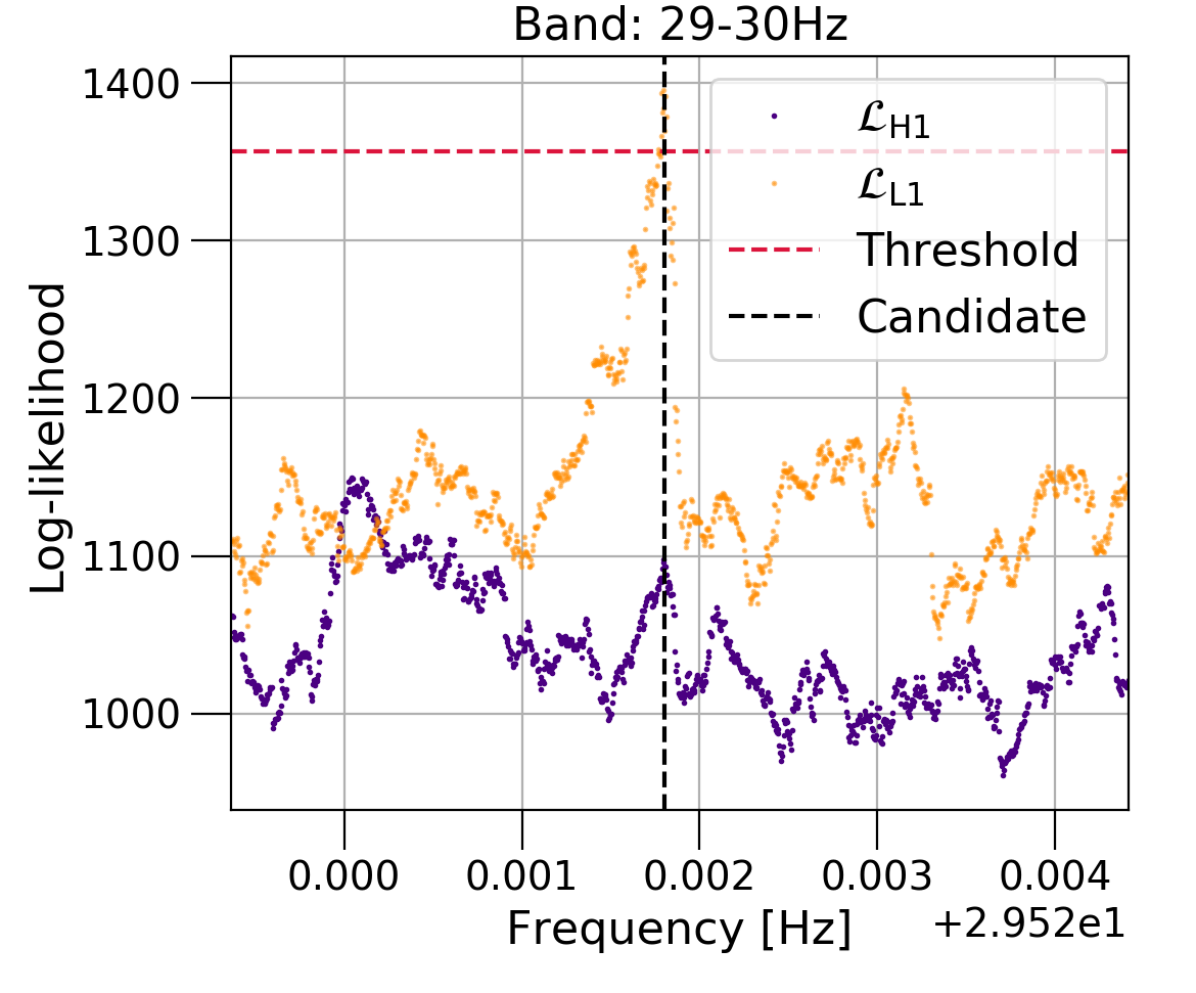
PSR J0534+2200: We search for a signal from this pulsar in the 29.530.5Hz (), 39.540.5Hz () and 59.560.5Hz () subbands. The search returns 11 candidates at , nine at and 12 at . Only one of these candidates survives the data quality vetoes.
-
1.
29.530.5Hz: The sole survivor in this subband is located on the peak of a spectral feature in the Livingston data and has , as shown in the top panel of Fig. 1. It also appears as a significant outlier in the Hanford only search with and in the offtarget search with 0.7. Since the candidate does not satisfy any of the veto criteria used here, we keep it for a followup study.
PSR J14206048: We search for a signal from this pulsar in the 1415Hz (), 1920Hz () and 2930Hz (2) subbands. The search returns 58 candidates at , 46 at and 35 at . Only one candidate survives the data quality vetoes in each subband.
-
1.
1415Hz: The candidate at 14.510Hz is more prominent in the Livingston data () than at Hanford (), as shown in the top panel of Fig. 2. It also resurfaces in the offtarget search with . Since the candidate does not satisfy any of the veto criteria used here, we keep it for a followup study.
-
2.
1920Hz: The sole survivor in this subband is more prominent in the Livingston data () than at Hanford (). It also resurfaces as a significant outlier in the offtarget search with , as shown in the bottom panel of Fig. 3. We keep the candidate for a followup study as it does not satisfy any of the veto criteria used here.
-
3.
2930Hz: The survivor at 29.5218Hz returns in the single IFO search and is shown in the top panel of Fig. 4. It also resurfaces as a significant outlier in the offtarget search with . Although it does not strictly satisfy any of the veto criteria used here, the relatively large in only one of the detectors, combined with a large points towards a nonastrophysical origin.


PSR J17183825: We look for a signal from this pulsar in the 1314Hz (), 17.518.5Hz () and 26.527.5Hz () subbands. The search returns 2051 candidates at , 165 at and 417 at . Only one candidate survives the data quality vetoes at , while none survive at or .
-
1.
17.518.5Hz: The sole candidate in this subband is visibly more prominent in the Hanford data than at Livingston, as shown in the top panel of Fig. 5. However, it has a comparable in both detectors (, ). The survivor also resurfaces in the offtarget search with . Although we keep this candidate for a followup study, its characteristics point towards a nonastrophysical origin.


PSR J1831-0953: We search for signals from this pulsar in 14.515.5Hz (), 19.520.5Hz () and 2930Hz () subbands. The search returns 1413 candidates at , 263 at and 81 at . Only two candidates survive the data quality vetoes at and , while none survive at .
-
1.
14.515.5Hz: The candidate at 14.50181Hz has and , as shown in Fig. 6. Although we keep this candidate for a followup study, the relatively large points toward a nonastrophysical origin. The second survivor at 15.40125Hz is more prominent in the Livingston data () than at Hanford (), as shown in Fig. 7. It also resurfaces in the offtarget search with . Although the candidate passes the data quality vetoes, its characteristics point towards a nonastrophysical origin.
-
2.
19.520.5Hz: The two survivors in this subband have frequency around 19.999Hz. Both have in the single IFO search, as shown in the top panel of Fig. 8. This could be explained by the fact that the Livingston detector is more sensitive than Hanford during O2 [93]. The candidates also show up in the offtarget search with . Since these candidates do not strictly satisfy any of the veto criteria, we keep them for a followup study. Despite this, their proximity to a spectral feature in the Livingston detector points towards a nonastrophysical origin.


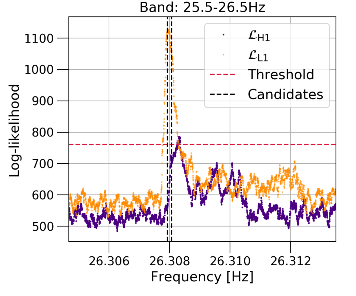
PSR J1849-0001: Search for a signal from this pulsar returns 57 candidates in the 25.526.5Hz () subband, 61 candidates at 3435Hz () and five in the 51.552.5Hz () subband. Only three candidates survive the data quality vetoes at , while none survive at or .
-
1.
25.526.5Hz: The first two survivors in this subband have frequency around Hz. Both have and , as shown in the top panel of Fig. 9. These candidates also survive the offtarget veto since they return . However, their characteristics point towards a nonastrophysical origin. The remaining candidate at 26.3410Hz is more prominent in the Livingston data () than at Hanford (), as shown in Fig. 10. It also survives the offtarget veto as it has . Despite this, the characteristics of the survivor as well as its proximity to a spectral feature in the Livingston detector points towards a nonastrophysical origin.


VII Conclusion
In this paper, we present a search for CW signals from ten pulsars selected on the basis of their highenergy emissions and association with TeV sources. The search uses publicly available data from the O2 run of the aLIGO detectors. We use a method which combines the maximumlikelihood statistic with a HMM to efficiently track the secular spindown and stochastic spin wandering of a CW signal. In addition to being fast, HMM has the ability to search a much wider set of histories than a coherent search with a Taylor series phase model, noting that the electromagnetic pulsations and CW signal are not necessarily locked together.
For each target, we scan 1Hz subbands around and and omit bands below 10Hz. Additionally, we choose a coherence timescale to ensure that the signal frequency falls within one frequency bin over a single coherent step. For all targets chosen for this search, the duration of the coherent segments is limited by the secular spindown () and not the stochastic spin wandering (). Despite this, it is vital to include stochastic spin wandering in the GW phase model because the CW signal may not be locked to the electromagnetic pulsations; the spin of the gravitationalwaveemitting quadrupole may wander invisibly a lot more than the electromagnetically timed solid crust.
The search returns a total of 5,256 candidates across 24 subbands. Only 12 candidates survive the three data quality vetoes outlined in Section V.5. Followup analysis indicates that seven candidates have and a single IFO loglikelihood (i.e., or ) which is comparable to . These survivors are marked with an asterisk in Table 5. Although these candidates survive the vetoes, their characteristics point towards a nonastrophysical origin. The remaining five candidates only exceed in the Livingston data and have . This is particularly true for the two survivors in 19.520.5Hz subband of PSR J18310953, both of which have and . However, we cannot reject these candidates purely on the basis of the outcome of single IFO veto, as Livingston is more sensitive than the Hanford detector during O2 [93].
A dedicated followup study using the method outlined here, but with data from the O3 run and future observing runs will provide further clarity on the nature of the remaining candidates. While we argue that the 12 candidates identified here are likely nonastrophysical in origin, they are potential signals and thus special care should be taken in following up on them. If they do prove to be from instrumental noise, future work should also consider additional vetoes that can be used to effectively rule out such artifacts.
A followup O3 search using the HMM will also provide an opportunity to undertake an injection study to determine upper limits. We do not attempt the exercise here because the phase model used in this paper (a biased random walk defined by the HMM’s transition probabilities) differs markedly from the phase models assumed in previous coherent CW searches for these targets (a Taylor series guided by the radio ephemeris). As upper limits are always conditional on the signal model used in the search, it is difficult to make an equivalent comparison. If the true GW signal is exactly locked (or nearly so) to the radio ephemeris, then a coherent search is more sensitive than the semicoherent HMM search by a factor in the characteristic wave strain [115, 116, 83, 87]. However, if the GW signal is displaced from the radio ephemeris and experiences significant spin wandering, a coherent search may miss the signal entirely, and the upper limits from the semicoherent HMM become decisive. In either scenario, the next significant step of placing constraints on the emission mechanism will be achieved once O3 data have been analysed.
Acknowledgements.
The authors would like to express their gratitude towards Ling Sun, Meg Millhouse, Hannah Middleton, Patrick Meyers, Lucy Strang and Julian Carlin for numerous discussions and their ongoing support throughout this project. Additionally, we extend our special thank you to Prof. Gavin Rowell for discussions of the various HESS targets. This research is supported by the Australian Research Council Centre of Excellence for Gravitational Wave Discovery (OzGrav) with project number CE170100004. This work was performed on the OzSTAR national facility at Swinburne University of Technology. The OzSTAR program receives funding in part from the Astronomy National Collaborative Research Infrastructure Strategy (NCRIS) allocation provided by the Australian Government. This research has made use of data, software and/or web tools obtained from the Gravitational Wave Open Science Center (https://www.gw-openscience.org/ ), a service of LIGO Laboratory, the LIGO Scientific Collaboration and the Virgo Collaboration. LIGO Laboratory and Advanced LIGO are funded by the United States National Science Foundation (NSF) as well as the Science and Technology Facilities Council (STFC) of the United Kingdom, the Max-Planck-Society (MPS), and the State of Niedersachsen/Germany for support of the construction of Advanced LIGO and construction and operation of the GEO600 detector. Additional support for Advanced LIGO was provided by the Australian Research Council. Virgo is funded, through the European Gravitational Observatory (EGO), by the French Centre National de Recherche Scientifique (CNRS), the Italian Istituto Nazionale di Fisica Nucleare (INFN) and the Dutch Nikhef, with contributions by institutions from Belgium, Germany, Greece, Hungary, Ireland, Japan, Monaco, Poland, Portugal, Spain.Appendix A Target parameters
Tables 6-15 outline the parameters used to search for CW signals from ten pulsars. Pulsars are named in the table titles. For each target, we report the reference time relevant to the measured ephemeris and bounds of the subbands at , and . The coherence timescale , number of transition steps , frequency resolution and the spindown rate measured via electromagnetic observations () are also reported. Finally, we quote the average onesided noise PSD for each subband of each target.
| Parameters | Search | Units | ||
|---|---|---|---|---|
| Ref time | 48442.5 | MJD | ||
| Band | 29.530.5 | 39.540.5 | 59.560.5 | Hz |
| 10.0 | 8.5 | 7 | hrs | |
| 560 | 659 | 801 | - | |
| 1.3889 | 1.6340 | 1.9841 | Hz | |
| -3.77535 | -5.03380 | -7.55070 | Hz | |
| S | 2.4 | 1.3 | 0.86 | Hzs-1 |
| Parameters | Search | Units | ||
|---|---|---|---|---|
| Ref time | 51559.319 | MJD | ||
| Band | 1112 | 14.515.5 | 2223 | Hz |
| 49.5 | 43 | 35 | hrs | |
| 113 | 130 | 160 | - | |
| 2.8058 | 3.2300 | 3.9683 | Hz | |
| -1.5666 | -2.0888 | -3.1332 | Hzs-1 | |
| S | 2.5 | 0.48 | 0.060 | Hzs-1 |
| Parameters | Search | Units | |
| Ref time | 52717.00000 | MJD | |
| Band | 1213 | 1819 | Hz |
| 64.0 | 52.0 | hrs | |
| 88 | 107 | - | |
| 2.1701 | 2.6455 | Hz | |
| -0.934620 | -1.40193 | Hzs-1 | |
| S | 1.5 | 0.18 | Hzs-1 |
| Parameters | Search | Units |
| Ref time | 52921.00000 | MJD |
| Band | 11.512.5 | Hz |
| 38.5 | hrs | |
| 146 | ||
| 3.6075 | Hz | |
| -2.610790 | Hzs-1 | |
| S | 2.3 | Hzs-1 |
| Parameters | Search | Units | ||
|---|---|---|---|---|
| Ref time | 51600.00 | MJD | ||
| Band | 1415 | 1920 | 2930 | Hz |
| 46.5 | 40 | 33 | hrs | |
| 121 | 140 | 170 | ||
| 2.9869 | 3.4722 | 4.2088 | Hz | |
| -1.78912 | -2.38549 | -3.57824 | Hzs-1 | |
| S | 5.1 | 1.2 | 0.25 | Hzs-1 |
| Parameters | Search | Units |
| Ref time | 55336 | MJD |
| Band | 12.513.5 | Hz |
| 17 | hrs | |
| 330 | ||
| 8.1699 | Hz | |
| -1.33062112 | Hzs-1 | |
| S | 1.2 | Hzs-1 |
| Parameters | Search | Units | ||
|---|---|---|---|---|
| Ref time | 51184.000 | MJD | ||
| Band | 1314 | 17.518.5 | 26.527.5 | Hz |
| 127.5 | 110.5 | 90 | hrs | |
| 44 | 51 | 62 | ||
| 1.0893 | 1.2569 | 1.5432 | Hz | |
| -2.371346 | -3.16179 | -4.742692 | Hzs-1 | |
| S | 8.0 | 2.5 | 0.3 | Hzs-1 |
| Parameters | Search | Units | |
| Ref time | 54200 | MJD | |
| Band | 12.513.5 | 1920 | Hz |
| 63 | 51.5 | hrs | |
| 89 | 109 | ||
| 2.2046 | 2.6969 | Hz | |
| -0.97417325 | -1.4612599 | Hzs-1 | |
| S | 1.2 | 0.12 | Hzs-1 |
| Parameters | Search | Units | ||
|---|---|---|---|---|
| Ref time | 52412.0000 | MJD | ||
| Band | 14.515.5 | 19.520.5 | 2930 | Hz |
| 145 | 125.5 | 102.5 | hrs | |
| 39 | 45 | 55 | ||
| 0.95785 | 1.1067 | 1.3550 | Hz | |
| -1.839595 | -2.452793 | -3.679190 | Hzs-1 | |
| S | 4.8 | 1.0 | 0.2 | Hzs-1 |
| Parameters | Search | Units | ||
|---|---|---|---|---|
| Ref time | 55535.285052933 | MJD | ||
| Band | 25.526.5 | 3435 | 51.552.5 | Hz |
| 63 | 55 | 44.5 | hrs | |
| 89 | 102 | 126 | ||
| 2.2046 | 2.5253 | 3.1210 | Hz | |
| -9.59 | -12.79 | -19.18 | Hzs-1 | |
| S | 3.4 | 1.5 | 0.90 | Hzs-1 |
Appendix B Spinwandering timescale
The strength of timing noise, inferred from timing the radio pulsation of a pulsar, is quantified by , the rms phase residual separating the actual signal and the best fit Taylor series which typically contains terms up to and including first frequency derivatives [97]. For random walks in rotation phase, frequency and spindown rate, the rms phase residual scales with the duration of the observation () as
| (28) |
where is a normalisation parameter and is the exponent of a powerlaw PSD used to model the observed timing noise [101, 102]. This powerlaw PSD is defined by
| (29) |
where, is the rednoise amplitude in units of and is the reference frequency of 1 cycle per year.
In this HMM search, the stochastic spin wandering timescale () is chosen such that the signal frequency falls in one frequency bin during a single coherent step. This sets the frequency resolution of the search to be
| (30) |
We also require the change in the signal frequency due to the stochastic spin wandering over [] to satisfy
| (31) |
where denotes the rms frequency residual used to estimate the scale of frequency wandering. We obtain an estimate for by differentiating Eq. 28 with respect to [103];
| (32) |
By combining Eqs. 30 and 32, we arrive at the following expression for , which depends on the parameters and .
| (33) |
We estimate for nine out of the ten pulsars in this study by first solving for parameter in Eq. 28. To do this, we estimate by
| (34) |
where denotes the rms timing residuals (in seconds) accumulated over a reference epoch used in the timing solution and denotes the star’s rotation frequency at the midpoint of this epoch. This combined with an appropriate choice of value for the parameter is then used to obtain an estimate for the normalisation parameter and thus .
We cannot find timing residuals for PSR J15135908 in the literature and thus estimate it using the fit parameters from its powerlaw PSD [102]
| (35) |
where, and are parameters as defined above, is the total observation time (in years) used to obtain a timing solution and is the reference timescale of 1 year.
The parameters used to estimate the stochastic spin wandering timescales for all pulsars are summarised in Table 16.
| Pulsar | Date Range | Res | Refs | ||||
|---|---|---|---|---|---|---|---|
| J2000] | [MJD] | [Hz] | [yrs] | [ms] | [Cycles] | [yrs] | |
| J05342200 | 4842248452 | 29.9466088403 | 0.082 | 0.1 | 0.003 | 1.902 | [117]333http://www.jb.man.ac.uk/pulsar/crab/crab2.txt |
| J08354510 | 5420055000 | 11.1856 | 2.19 | 440 | 4.922 | 0.609 | [118] |
| J10165857 | 5145152002 | 9.31274229245(4) | 1.51 | 4.3 | 0.0401 | 2.87 | [119] |
| J13576429 | 5348753714 | 6.019298216(5) | 0.62 | 3.6 | 0.0217 | 1.51 | [120] |
| J14206048 | 5420054600 | 14.66275659824 | 1.09 | 70 | 1.02 | 0.57 | [118] |
| J15135908 | 5422058469 | 6.59709182778(19) | 11.6 | 298.2 | 1.97 | 4.52 | [102] |
| J17183825 | 5420055000 | 13.386880856760 | 2.19 | 27 | 0.361 | 1.73 | [118] |
| J18261334 | 48486.4-52793.4 | 9.856 | 11.8 | 2267.62 | 22.35 | 1.79 | [21] |
| J18310952 | 5130253523 | 14.8661645038(14) | 6 | 2.0 | 0.0297 | 13.04 | [121] |
| J18490001 | 58166.458355.9 | 25.9590178660(19) | 0.52 | 0.525 | 0.0136 | 1.52 | [122] |
Appendix C Offtarget veto
Here, we outline the procedure used to select an appropriate offset for the offtarget veto. It is based on injecting signals into the aLIGO O2 data. To simplify the study, we use the same search parameters as the ones used in the 59.560.5Hz subband of PSR J05342200. The source and search parameters are outlined in Tables 17 and 18. We conservatively use a coherence time of 7hrs for this study since shorter coherence times exhibit less sensitivity to sky position, as the Earth experiences less diurnal motion.
| Parameters | Value | Units |
|---|---|---|
| 1 | - | |
| [0, ) | rad | |
| 0.3842248 | rad | |
| 2.5 | - | |
| 7 | hrs | |
| 233.6 | days |
| Parameters | Value | Units |
|---|---|---|
| Band | 59.560.5 | Hz |
| + | rad | |
| + | rad | |
| 7 | hrs | |
| 801 | - | |
| 1.9841 | Hz | |
| -7.55070 | Hz |
Here, we experiment with three different values of , the offset in right ascension of the search from source’s location. These include of 0.262 rad (1hr), 0.524 rad (2hrs) and 0.785 rad (3hrs). In each case, we set (i.e., the offset in search declination) to 0.003 rad (10min). Note that the because the response of the two detectors changes with , which would artificially adjust of the recovered signal [19]. For each , we repeat the following procedure for 100 realisations.
-
1.
Generate a fake signal: The parameters of the injected signal are outlined in Table 17. We use , which corresponds to the upper limit on the detectable signal () for this subband. Additionally, we generate a Viterbi path where the signal frequency follows a biased random walk as described by the transition matrix in Eq. 20 of Section IV.3.
-
2.
Inject signal in LIGO data: We use the lalappsMakefakedatav4 tool in the LAL suite [109] to inject fake signals into the Hanford and Livingston detector data. To randomise the search between each run, we sample (i.e., right ascension of the source) from a uniform distribution of values between [0, 2) while fixing rad from EM measurements (i.e., ).
-
3.
Search for the injected signal: We search for the injected signal in O2 data using a combination of the statistic and Viterbi algorithm. As shown in Fig. 11, this LIGO subband is contaminated by noise lines. Therefore, we choose to restrict the analysis to a 0.2Hz wide region around the injected signal frequency. The search is then performed at an ontarget (i.e., at the same location as the injected signal) and offtarget sky position.
-
4.
Compare results: We compare loglikelihood and Viterbi path of the candidate from the on and offtarget searches. The two Viterbi paths are classified as overlapping if the offtarget path lies within the extended ontarget path, which accounts for the frequency shift expected due to the Doppler modulation of the Earth.

The outcomes of the injection studies are presented in Fig. 12. We plot against for three cases. The top panel shows the results for the case where the search is offset from the source’s location by () in right ascension and declination, respectively. The search returns candidates with 95 of the time. This is problematic if the offtarget veto criterion is based on comparing with , as is the case in Ref. [88]. This offset and veto criterion would incorrectly reject astrophysical signals 95 of the time. Additionally, both on and offtarget searches return comparable , as most of the data points lie along to the line. Hence we cannot safely discern between an astrophysical signal and a noise artifact in the detector, which would be expected to produce comparable in on and offtarget searches.
The middle panel shows the results for the case where the offtarget search is offset from the source’s location by () in right ascension and declination. Approximately 67 of the abovethreshold, ontarget candidates are subthreshold in the offtarget search. Although this is significantly better than the above case, the offtarget veto would incorrectly reject approximately 33 of the true astrophysical signals, provided the criterion is set to reject candidates with . None of the candidates in this search have . This implies that this offtarget offset would produce a noticeable (but not significant) change in of an astrophysical candidate. Therefore, it may still be difficult to discern a true astrophysical signal from a noise artifact.
We show the results for a search offset of () in the bottom panel of Fig. 12. The crosses indicate the Viterbi paths which do not overlap since the recovered offtarget path doesn’t lie within the extended ontarget path, which accounts for the Doppler modulation of the Earth. In three out of five cases, this occurs because of the injected signals is comparable to the background noise. Since the algorithm backtracks the Viterbi path with the highest in a 0.2Hz wide region around the injected signal frequency, a nonoverlapping Viterbi path is recovered in the offtarget search. In the remaining two cases, the recovered path lies just outside the extended ontarget path and thus deemed to be nonoverlapping. The results here clearly indicate that this offset should reduce for an astrophysical signal. This should be sufficient to easily distinguish between an astrophysical signal and a noise artifact, which is expected to produce comparable in both on and offtarget searches. Additionally, we can also compare with for candidates that are marginally abovethreshold in the ontarget search. This is because the offset should yield for signals close to the Gaussian threshold.
Based on these results, we conclude that an offset of in right ascension and in declination for the offtarget search should produce a noticeable change in of an astrophysical signal. Our most conservative estimates suggest that with this offset, a real signal would produce . Additionally, searches with longer coherence times would be expected to produce significantly lower . Therefore, we choose to reject candidates with in this study. This should reject noise lines without unduly affecting the false alarm or false dismissal probabilities.


Appendix D Candidates
Figs. 13-22 show the results for 24 subbands explored in this study. For each subband, we plot the loglikelihood () against the terminating frequency of the associated Viterbi path. Candidates are overlaid along with the outcome at each stage of the data quality vetoes. We discuss the characteristics of veto 3 survivors (indicated by blue stars) in Section VI.1.


References
- Abbott et al. [2019a] B. P. Abbott et al. (LIGO Scientific and Virgo Collaborations), GWTC-1: A Gravitational-Wave Transient Catalog of Compact Binary Mergers Observed by LIGO and Virgo during the First and Second Observing Runs, Phys. Rev. X 9, 031040 (2019a).
- Aasi et al. [2015a] J. Aasi et al. (LIGO Scientific Collaboration), Advanced LIGO, Classical Quantum Gravity 32, 074001 (2015a).
- Acernese et al. [2014] F. Acernese et al., Advanced Virgo: A second-generation interferometric gravitational wave detector, Classical Quantum Gravity 32, 024001 (2014).
- Abbott et al. [2016a] B. P. Abbott et al. (LIGO Scientific and Virgo Collaboration), Observation of Gravitational Waves from a Binary Black Hole Merger, Phys. Rev. Lett. 116, 061102 (2016a).
- Abbott et al. [2016b] B. P. Abbott et al., GW151226: Observation of Gravitational Waves from a 22-Solar-Mass Binary Black Hole Coalescence, Phys. Rev. Lett. 116, 241103 (2016b).
- Abbott et al. [2017a] B. P. Abbott et al., GW170814: A Three-Detector Observation of Gravitational Waves from a Binary Black Hole Coalescence, Phys. Rev. Lett. 119, 141101 (2017a).
- Abbott et al. [2017b] B. P. Abbott et al., GW170817: Observation of Gravitational Waves from a Binary Neutron Star Inspiral, Phys. Rev. Lett. 119, 161101 (2017b).
- Abbott et al. [2017c] B. P. Abbott et al., Multi-messenger observations of a binary neutron star merger, Astrophys. J. 848, L12 (2017c).
- Riles [2013] K. Riles, Gravitational waves: Sources, detectors and searches, Prog. Part. Nucl. Phys. 68, 1 (2013).
- Riles [2017] K. Riles, Recent searches for continuous gravitational waves, Mod. Phys. Lett. A 32, 1730035 (2017).
- Mastrano et al. [2013] A. Mastrano, P. Lasky, and A. Melatos, Neutron star deformation due to multipolar magnetic fields, Mon. Not. Roy. Astron. Soc. 434, 1658 (2013).
- Ushomirsky et al. [2000] G. S. Ushomirsky, C. Cutler, and L. Bildsten, Deformations of accreting neutron star crusts and gravitational wave emission, Mon. Not. R. Astron. Soc. 319, 902 (2000).
- Melatos and Payne [2005] A. Melatos and D. Payne, Gravitational radiation from an accreting millisecond pulsar with a magnetically confined mountain, Astrophys. J. 623, 1044 (2005).
- Owen et al. [1998] B. J. Owen, L. Lindblom, C. Cutler, B. F. Schutz, A. Vecchio, and N. Andersson, Gravitational waves from hot young rapidly rotating neutron stars, Phys. Rev. D 58, 084020 (1998).
- Jones and Andersson [2001] D. I. Jones and N. Andersson, Freely precessing neutron stars: model and observations, Mon. Not. R. Astron. Soc. 324, 811 (2001).
- Wette et al. [2018] K. Wette, S. Walsh, R. Prix, and M. A. Papa, Implementing a semicoherent search for continuous gravitational waves using optimally-constructed template banks, Phys. Rev. D 97, 123016 (2018).
- Jones [2015] D. I. Jones, Parameter choices and ranges for continuous gravitational wave searches for steadily spinning neutron stars, Mon. Not. R. Astron. Soc. 453, 53 (2015).
- Wette [2012] K. Wette, Estimating the sensitivity of wide-parameter-space searches for gravitational-wave pulsars, Phys. Rev. D 85, 042003 (2012).
- Jaranowski et al. [1998] P. Jaranowski, A. Krolak, and B. F. Schutz, Data analysis of gravitational-wave signals from spinning neutron stars. I. The signal and its detection, Phys. Rev. D 58, 063001 (1998).
- Prix and Shaltev [2012] R. Prix and M. Shaltev, Search for continuous gravitational waves: Optimal StackSlide method at fixed computing cost, Phys. Rev. D 85, 084010 (2012).
- Hobbs et al. [2010] G. Hobbs, A. G. Lyne, and M. Kramer, An analysis of the timing irregularities for 366 pulsars, Mon. Not. R. Astron. Soc. 402, 1027 (2010).
- Ashton et al. [2015] G. Ashton, D. I. Jones, and R. Prix, Effect of timing noise on targeted and narrow-band coherent searches for continuous gravitational waves from pulsars, Phys. Rev. D 91, 062009 (2015).
- Suvorova et al. [2017] S. Suvorova, P. Clearwater, A. Melatos, L. Sun, W. Moran, and R. J. Evans, Hidden Markov model tracking of continuous gravitational waves from a binary neutron star with wandering spin. II. Binary orbital phase tracking, Phys. Rev. D 96, 102006 (2017).
- Lyne et al. [2010] A. Lyne, G. Hobbs, M. Kramer, I. Stairs, and B. Stappers, Switched magnetospheric regulation of pulsar spin-down, Science 329, 408 (2010).
- Janssen and Stappers [2006] G. H. Janssen and B. W. Stappers, 30 glitches in slow pulsars, Astron. Astrophys. 457, 611 (2006).
- Price et al. [2012] S. Price, B. Link, S. Shore, and D. Nice, Time-correlated structure in spin fluctuations in pulsars, Mon. Not. R. Astron. Soc. 426, 2507 (2012).
- Melatos and Link [2014] A. Melatos and B. Link, Pulsar timing noise from superfluid turbulence, Mon. Not. R. Astron. Soc. 437, 21 (2014).
- Cheng [1987] K. S. Cheng, Could glitches inducing magnetospheric fluctuations produce low-frequency pulsar timing noise?, Astrophys. J. 321, 805 (1987).
- Urama et al. [2006] J. O. Urama, B. Link, and J. M. Weisberg, A strong correlation in radio pulsars with implications for torque variations, Mon. Not. R. Astron. Soc. Lett. 370, L76 (2006).
- Arzoumanian et al. [1994] Z. Arzoumanian, D. Nice, J. Taylor, and S. Thorsett, Timing behavior of 96 radio pulsars, Astrophys. J. 422, 671 (1994).
- Quinn and Hannan [2001] B. G. Quinn and E. J. Hannan, The Estimation and Tracking of Frequency, Cambridge Series in Statistical and Probabilistic Mathematics (Cambridge University Press, Cambridge, England, 2001).
- Dreissigacker et al. [2018] C. Dreissigacker, R. Prix, and K. Wette, Fast and accurate sensitivity estimation for continuous-gravitational-wave searches, Phys. Rev. D 98, 084058 (2018).
- Abbott et al. [2008] B. P. Abbott et al., Beating the spin-down limit on gravitational wave emission from the Crab pulsar, The Astrophysical Journal 683, L45 (2008).
- Abbott et al. [2005] B. P. Abbott et al. (LIGO Scientific Collaboration), Limits on Gravitational-Wave Emission from Selected Pulsars Using LIGO Data, Phys. Rev. Lett. 94, 181103 (2005).
- Abbott et al. [2007] B. P. Abbott et al. (LIGO Scientific Collaboration), Upper limits on gravitational wave emission from 78 radio pulsars, Phys. Rev. D 76, 042001 (2007).
- Abbott et al. [2010] B. P. Abbott et al., Searches for gravitational waves from known pulsars with science run 5 LIGO data, Astrophys. J. 713, 671 (2010).
- Abadie et al. [2011] J. Abadie et al. (LIGO Scientific and Virgo Collaborations), Beating the spin-down limit on gravitational wave emission from the Vela pulsar, Astrophys. J. 737, 93 (2011).
- Aasi et al. [2014] J. Aasi et al., Gravitational waves from known pulsars: Results from the initial detector era, Astrophys. J. 785, 119 (2014).
- Aasi et al. [2015b] J. Aasi et al. (LIGO Scientific and Virgo Collaborations), Narrow-band search of continuous gravitational-wave signals from Crab and Vela pulsars in Virgo VSR4 data, Phys. Rev. D 91, 022004 (2015b).
- Abbott et al. [2017d] B. P. Abbott et al. (LIGO Scientific and Virgo Collaborations), First narrow-band search for continuous gravitational waves from known pulsars in advanced detector data, Phys. Rev. D 96, 122006 (2017d).
- Abbott et al. [2017e] B. P. Abbott et al., First search for gravitational waves from known pulsars with advanced LIGO, Astrophys. J. 839, 12 (2017e).
- Abbott et al. [2019b] B. P. Abbott et al. (LIGO Scientific and Virgo Collaborations), Narrow-band search for gravitational waves from known pulsars using the second LIGO observing run, Phys. Rev. D 99, 122002 (2019b).
- Abbott et al. [2019c] B. P. Abbott et al., Searches for gravitational waves from known pulsars at two harmonics in 2015-2017 LIGO data, Astrophys. J. 879, 10 (2019c).
- Cui [2009] W. Cui, TeV gamma-ray astronomy, Res. Astron. Astrophys. 9, 841 (2009).
- Holder [2012] J. Holder, Tev gamma-ray astronomy: A summary, Astropart. Phys. 39-40, 61 (2012).
- Abdalla et al. [2018a] H. Abdalla et al. (HESS Collaboration), The population of TeV pulsar wind nebulae in the H.E.S.S. Galactic plane survey, Astron. Astrophys. 612, A2 (2018a).
- Grenier and Harding [2015] I. A. Grenier and A. K. Harding, Gamma-ray pulsars: A gold mine, C. R. Phys. 16, 641 (2015).
- Bai and Spitkovsky [2010] X. Bai and A. Spitkovsky, Modelling of gamma-ray pulsar light curves using the force-free magnetic fields, Astrophys. J. 715, 1282 (2010).
- Chugunov and Horowitz [2010] A. I. Chugunov and C. J. Horowitz, Breaking stress of neutron star crust, Mon. Not. R. Astron. Soc. Lett. 407, L54 (2010).
- Knispel and Allen [2008] B. Knispel and B. Allen, Blandford’s argument: The strongest continuous gravitational wave signal, Phys. Rev. D 78, 044031 (2008).
- Wette et al. [2010] K. Wette, M. Vigelius, and A. Melatos, Sinking of a magnetically confined mountain on an accreting neutron star, Mon. Not. R. Astron. Soc. 402, 1099 (2010).
- Harding and Muslimov [1998] A. K. Harding and A. G. Muslimov, Particle acceleration zones above pulsar polar caps: Electron and positron pair formation fronts, Astrophys. J. 508, 328 (1998).
- Harding and Muslimov [2002] A. K. Harding and A. Muslimov, Pulsar polar cap heating and surface thermal x-ray emission. II. Inverse Compton radiation pair fronts, Astrophys. J. 568, 862 (2002).
- Levinson et al. [2005] A. Levinson, D. Melrose, A. Judge, and Q. Luo, Large-amplitude, pair-creating oscillations in pulsar and black hole magnetospheres, Astrophys. J. 631, 456 (2005).
- Muslimov and Harding [2003] A. G. Muslimov and A. K. Harding, Extended acceleration in slot gaps and pulsar high-energy emission, Astrophys. J. 588, 430 (2003).
- Abdalla et al. [2018b] H. Abdalla et al., The H.E.S.S. Galactic plane survey, Astron. Astrophys. 612, A1 (2018b).
- Pitkin [2011] M. Pitkin, Prospects of observing continuous gravitational waves from known pulsars, Mon. Not. R. Astron. Soc. 415, 1849 (2011).
- Note [1] http://tevcat2.uchicago.edu/.
- Vigelius et al. [2007] M. Vigelius, A. Melatos, S. Chatterjee, B. M. Gaensler, and P. Ghavamian, Three-dimensional hydrodynamic simulations of asymmetric pulsar wind bow shocks, Mon. Not. R. Astron. Soc. 374, 793 (2007).
- Manchester et al. [2005] R. N. Manchester, G. B. Hobbs, A. Teoh, and M. Hobbs, The Australia Telescope National Facility Pulsar Catalogue, Astrophys. J. 129, 1993 (2005).
- Cordes and Lazio [2002] J. M. Cordes and T. J. W. Lazio, NE2001.I. A New Model for the Galactic Distribution of Free Electrons and its Fluctuations, arXiv e-prints , astro-ph/0207156 (2002), arXiv:astro-ph/0207156 [astro-ph] .
- Lyne et al. [2006] A. Lyne, F. Graham-Smith, and F. Graham-Smith, Pulsar Astronomy, Cambridge Astrophysics (Cambridge University Press, Cambridge, England, 2006).
- Gotthelf et al. [2011] E. Gotthelf, J. Halpern, R. Terrier, and F. Mattana, Discovery of an energetic 38.5 ms pulsar powering the gamma-ray source IGR J18490-0000/HESS J1849-000, Astrophys. J. 729, L16 (2011).
- Abdo et al. [2009] A. Abdo et al., Fermi large area telescope observations of the crab pulsar and nebula, Astrophys. J. 708, 1254 (2009).
- Aliu et al. [2011] E. Aliu et al., Detection of pulsed gamma rays above 100 GeV from the Crab pulsar, Science 334, 69–72 (2011).
- Venter et al. [2018] C. Venter, A. Harding, and I. Grenier, High-energy emission properties of pulsars, Proc. Sci. MULTIF2017, 038 (2018).
- Abdo et al. [2010] A. A. Abdo et al., The Vela pulsar: Results from the first year of Fermi-LAT observations, Astrophys. J. 713, 154 (2010).
- Abdalla et al. [2018c] H. Abdalla, F. Aharonian, F. Ait Benkhali, E. O. Angüner, M. Arakawa, C. Arcaro, C. Armand, M. Arrieta, M. Backes, et al., First ground-based measurement of sub-20 GeV to 100 GeV -Rays from the Vela pulsar with H.E.S.S. II, Astron. Astrophys. 620, A66 (2018c).
- Abramowski et al. [2015] A. Abramowski, F. Aharonian, et al., Discovery of variable VHE -ray emission from the binary system 1FGL J1018.6-5856, Astron. Astrophys. 577, A131 (2015).
- Acero et al. [2013] F. Acero et al., Constraints on the galactic population of TeV pulsar wind nebulae using fermi large area telescope observations, Astrophys. J. 773, 77 (2013).
- Abramowski et al. [2011] A. Abramowski et al., Discovery of the source HESS J1356-645 associated with the young and energetic PSR J1357-6429, Astron. Astrophys. 533, A103 (2011).
- de los Reyes et al. [2012] R. de los Reyes, A. Zajczyk, and R. C. G. Chaves (HESS Collaboration), A newly discovered VHE gamma-ray PWN candidate around PSR J1459-60, arXiv e-prints , arXiv:1205.0719 (2012), arXiv:1205.0719 [astro-ph.HE] .
- Roberts et al. [2001] M. S. E. Roberts, R. W. Romani, and S. Johnston, Multi-wavelength Studies of PSR J1420-6048, a young pulsar in the Kookaburra, Astrophys. J. 561, L187 (2001).
- Aharonian et al. [2005] F. Aharonian, A. G. Akhperjanian, et al., Discovery of extended VHE gamma-ray emission from the asymmetric pulsar wind nebula in MSH 15-52 with HESS, Astron. Astrophys. 435, L17 (2005).
- Tsirou et al. [2018] M. Tsirou, Y. Gallant, R. Zanin, and R. Terrier (H.E.S.S.), VHE gamma-ray study of the composite SNR MSH 15-52 with H.E.S.S, Proc. Sci. ICRC2017, 681 (2018), arXiv:1709.01422 .
- Hinton et al. [2007] J. A. Hinton, S. Funk, S. Carrigan, Y. A. Gallant, O. C. de Jager, K. Kosack, A. Lemière, and G. Pühlhofer, Discovery of an x-ray nebula around PSR J1718-3825 and implications for the nature of the gamma-ray source HESS-J1718-385, Astron. Astrophys. 476, L25 (2007).
- Mitchell et al. [2018] A. Mitchell, S. Caroff, R. D. Parsons, J. Hahn, V. Marandon, and J. Hinton (HESS Collaboration), Observations of the pulsar wind nebula HESS J1825-137 with H.E.S.S. II, Proc. Sci. ICRC2017, 707 (2018).
- Duvidovich et al. [2019] L. Duvidovich et al., A new study towards PSR J1826-1334 and PSR J1826-1256 in the region of HESS J1825-137 and HESS J1826-130, Astron. Astrophys. 623, A115 (2019).
- Linden et al. [2017] T. Linden, K. Auchettl, J. Bramante, I. Cholis, K. Fang, D. Hooper, T. Karwal, and S. W. Li, Using hawc to discover invisible pulsars, Phys. Rev. D 96, 103016 (2017).
- Sheidaei et al. [2011] F. Sheidaei, A. Djannati-Ataï, and H. Gast (H.E.S.S.), Discovery of very-high-energy -ray emission from the vicinity of PSR J1831-952 with H.E.S.S., in Proceedings of the 3rd International Cosmic Ray Conference (ICRC2011) (2011) pp. 244–247, arXiv:1110.6837 .
- Abeysekara et al. [2017] A. U. Abeysekara et al., The 2HWC HAWC observatory gamma-ray catalog, Astrophys. J. 843, 40 (2017).
- Vleeschower Calas et al. [2018] L. Vleeschower Calas, S. Kaufmann, C. Alvarez Ochoa, and O. Tibolla, Studies of high-energy pulsars: The special case of PSR J1849-0001, Nucl. Part. Phys. Proc. 297-299, 102 (2018).
- Abbott et al. [2017f] B. P. Abbott et al. (LIGO Scientific and Virgo Collaborations), Search for gravitational waves from Scorpius X-1 in the first Advanced LIGO observing run with a hidden Markov model, Phys. Rev. D 95, 122003 (2017f).
- Henderson et al. [1997] J. Henderson, S. Salzberg, and K. H. Fasman, Finding genes in DNA with a hidden markov model, J. Comput. Biol. 4, 127 (1997).
- Tugac and Efe [2012] S. Tugac and M. Efe, Radar target detection using hidden Markov models, Prog. Electromagn. Res. B 44, 241 (2012).
- Nefian and Hayes [1998] A. V. Nefian and M. H. Hayes, Hidden Markov Models for Face Recognition, in Proceedings of the 1998 IEEE International Conference on Acoustics, Speech and Signal Processing, ICASSP ’98 (Cat. No.98CH36181), Vol. 5 (1998) pp. 2721–2724 vol.5.
- Abbott et al. [2019d] B. P. Abbott et al., Search for gravitational waves from Scorpius X-1 in the second Advanced LIGO observing run with an improved hidden Markov model, Phys. Rev. D 100, 122002 (2019d).
- Middleton et al. [2020] H. Middleton, P. Clearwater, A. Melatos, and L. Dunn, Search for gravitational waves from five low mass x-ray binaries in the second Advanced LIGO observing run with an improved hidden Markov model, Phys. Rev. D 102, 023006 (2020).
- Sun et al. [2018] L. Sun, A. Melatos, S. Suvorova, W. Moran, and R. J. Evans, Hidden Markov model tracking of continuous gravitational waves from young supernova remnants, Phys. Rev. D 97, 043013 (2018).
- Sun and Melatos [2019] L. Sun and A. Melatos, Application of hidden Markov model tracking to the search for long-duration transient gravitational waves from the remnant of the binary neutron star merger GW170817, Phys. Rev. D 99, 123003 (2019).
- Suvorova et al. [2016] S. Suvorova, L. Sun, A. Melatos, W. Moran, and R. J. Evans, Hidden Markov model tracking of continuous gravitational waves from a neutron star with wandering spin, Phys. Rev. D 93, 123009 (2016).
- Bellman [1966] R. Bellman, Dynamic programming, Science 153, 34 (1966).
- Abbott et al. [2021] R. Abbott et al. (LIGO Scientific and Virgo Collaborations), Open data from the first and second observing runs of advanced ligo and advanced virgo, SoftwareX 13, 100658 (2021), https://www.gw-openscience.org/O2/.
- Link and Epstein [1991] B. Link and R. Epstein, Mechanics and energetics of vortex unpinning in neutron stars, Astrophys. J. 373, 592 (1991).
- Melatos [2012] A. Melatos, Fast fossil rotation of neutron star cores, Astrophys. J. 761, 32 (2012).
- Cahillane et al. [2017] C. Cahillane et al., Calibration uncertainty for Advanced LIGO’s first and second observing runs, Phys. Rev. D 96, 102001 (2017).
- Jones [2004] D. I. Jones, Is timing noise important in the gravitational wave detection of neutron stars?, Phys. Rev. D 70, 042002 (2004).
- Lyne et al. [2015] A. G. Lyne et al., 45 years of rotation of the Crab pulsar, Mon. Not. R. Astron. Soc. 446, 857 (2015).
- Ferrari and Ruffini [1969] A. Ferrari and R. Ruffini, Theoretical implications of the second time derivative of the period of the pulsar NP 0532, Astrophys. J. 158, L71 (1969).
- Phillips and Thorsett [1994] J. A. Phillips and S. E. Thorsett, Planets around pulsars: A review, in Planetary Systems: Formation, Evolution, and Detection, edited by B. F. Burke, J. H. Rahe, and E. E. Roettger (Springer Netherlands, Dordrecht, 1994) pp. 91–106.
- Shannon et al. [2016] R. M. Shannon et al., Characterizing the rotational irregularities of the Vela pulsar from 21yr of phase-coherent timing, Mon. Not. R. Astron. Soc. 459, 3104 (2016).
- Parthasarathy et al. [2019] A. Parthasarathy et al., Timing of young radio pulsars - I. Timing noise, periodic modulation, and proper motion, Mon. Not. R. Astron. Soc. 489, 3810 (2019).
- Cordes [1980] J. Cordes, Pulsar timing. II. Analysis of random walk timing noise : Application to the Crab pulsar., Astrophys. J. 237, 216 (1980).
- Espinoza et al. [2011] C. M. Espinoza et al., A study of 315 glitches in the rotation of 102 pulsars, Mon. Not. R. Astron. Soc. 414, 1679 (2011).
- Haskell and Melatos [2015] B. Haskell and A. Melatos, Models of pulsar glitches, Int. J. Mod. Phys. D 24, 1530008 (2015).
- Note [2] http://www.jb.man.ac.uk/pulsar/glitches.html.
- Basu et al. [2019] A. Basu et al., Observed glitches in eight young pulsars, Mon. Not. R. Astron. Soc. 491, 3182 (2019).
- Palfreyman et al. [2018] J. Palfreyman, J. Dickey, et al., Alteration of the magnetosphere of the vela pulsar during a glitch, Nature 556 (2018).
- LIGO Scientific Collaboration [2018] LIGO Scientific Collaboration, LIGO Algorithm Library - LALSuite, free software (GPL) (2018).
- Covas et al. [2018] P. B. Covas et al. (LSC Instrument Authors), Identification and mitigation of narrow spectral artifacts that degrade searches for persistent gravitational waves in the first two observing runs of Advanced LIGO, Phys. Rev. D 97, 082002 (2018).
- Jones and Sun [2021] D. Jones and L. Sun, Search for continuous gravitational waves from Fomalhaut b in the second Advanced LIGO observing run with a hidden Markov model, Phys. Rev. D 103, 023020 (2021).
- Isi et al. [2020] M. Isi et al., Establishing the significance of continuous gravitational-wave detections from known pulsars, Phys. Rev. D 102, 123027 (2020).
- [113] R. Abbott et al. (LIGO Scientific and Virgo Collaborations), Searches for continuous gravitational waves from young supernova remnants in the early third observing run of Advanced LIGO and Virgo, to be published.
- Caride et al. [2019] S. Caride, R. Inta, B. J. Owen, and B. Rajbhandari, How to search for gravitational waves from r-modes of known pulsars, Phys. Rev. D 100, 064013 (2019).
- Dhurandhar et al. [2008] S. Dhurandhar, B. Krishnan, H. Mukhopadhyay, and J. T. Whelan, Cross-correlation search for periodic gravitational waves, Phys. Rev. D 77, 082001 (2008).
- Aasi et al. [2015c] J. Aasi et al. (LIGO Scientific and Virgo Collaborations), Directed search for gravitational waves from Scorpius X-1 with initial LIGO data, Phys. Rev. D 91, 062008 (2015c).
- Lyne et al. [1993] A. G. Lyne, R. S. Pritchard, and F. Graham Smith, 23 years of Crab pulsar rotational history, Mon. Not. R. Astron. Soc. 265, 1003 (1993).
- Weltevrede et al. [2010] P. Weltevrede et al., Pulsar timing with the Parkes radio telescope for the fermi mission, Publ. Astron. Soc. Aust. 27, 64 (2010).
- Camilo et al. [2001] F. Camilo et al., PSR J1016-5857: A young radio pulsar with possible supernova remnant, x-ray, and gamma-ray associations, Astrophys. J. 557, L51 (2001).
- Zavlin [2007] V. E. Zavlin, First x-ray observations of the young Pulsar J1357-6429, Astrophys. J. 665, L143 (2007).
- Lorimer et al. [2006] D. R. Lorimer et al., The parkes multibeam pulsar survey - VI. Discovery and timing of 142 pulsars and a galactic population analysis, Mon. Not. R. Astron. Soc. 372, 777 (2006).
- Bogdanov et al. [2019] S. Bogdanov, W. C. G. Ho, T. Enoto, S. Guillot, A. Harding, G. K. Jaisawal, C. Malacaria, S. S. Manthripragada, Z. Arzoumanian, and K. Gendreau, NICER X-ray Timing of Radio and Gamma-ray Quiet Pulsars for Continuous Gravitational Wave Source Searches, Astrophys. J. 877, 69 (2019).