SDSS-IV MaNGA: The [$\alpha$/Fe] of Early-Type Galaxies

The data for our analysis in this work are from the SDSS Data Release 15 (DR15), MaNGA Product Launch 7 (MPL7). All raw MaNGA data are firstly reduced by the Data Reduction Pipeline (DRP; Law et al., 2016). Then these science-ready data cubes are analysed by the Data Analysis Pipeline (DAP; Westfall et al., 2019). In this step, DAP spatially bins the data cubes in a certain way, and measure the physical parameters from the stacked spectrum in each bin. Our work is based on the DAP products. The binning method we adopted is the Voronoi binning (Cappellari & Copin, 2003) at a target S/N of 10.

DAP produces both the three dimensional LOGCUBE files and the two dimensional MAPS files. The LOGCUBE files are similar to the DRP cubes. Behind each spaxel in LOGCUBE files, the spectra in different dimensions correspond to either the spectrum stacked from the bin it belongs to or the fitting outputs from this stacked spectrum. The MAPS files record a range of parameters that are measured from the corresponding spectra in DAP cubes.

Li et al. (2018, hereafter L18) estimated the velocity dispersions within 1R_e ($\sigma_{e}$) of MaNGA MPL5 galaxies by dynamical modelling. We adopt their $\sigma_{e}$ measurements and take the MPL5 galaxies as our parent sample. L18 also provided the morphological classification of these galaxies, which was based on the GalaxyZoo project (Lintott et al., 2008, 2011). We adopt this traditional classification to select out ETGs, so that our results are comparable to most previous studies in this field (Cappellari, 2016).

For the purpose of studying high-S/N spectra, we only select the ETGs with the median S/N within 1R_e higher than 30. The median S/N within 1R_e is provided by DAP MAPS files. This criterion ensures the S/N of our binned spectra all above 50 and mostly higher than 80 (See Figure 2 and further description in §3.1), high enough for a relatively accurate spectral fitting analysis (see §4.1). Because we check the representativeness of our sample by means of the Lick index analysis (§4.3), our sample only includes the galaxies with all the related indices (Fe4383, Mg$b$, Fe5270, Fe5335) available. These galaxies also have useable H_β index for age estimations. Under these criteria, our sample contains 196 ETGs. Their $\sigma_{e}$ ranges from 27 to 270 km/s.

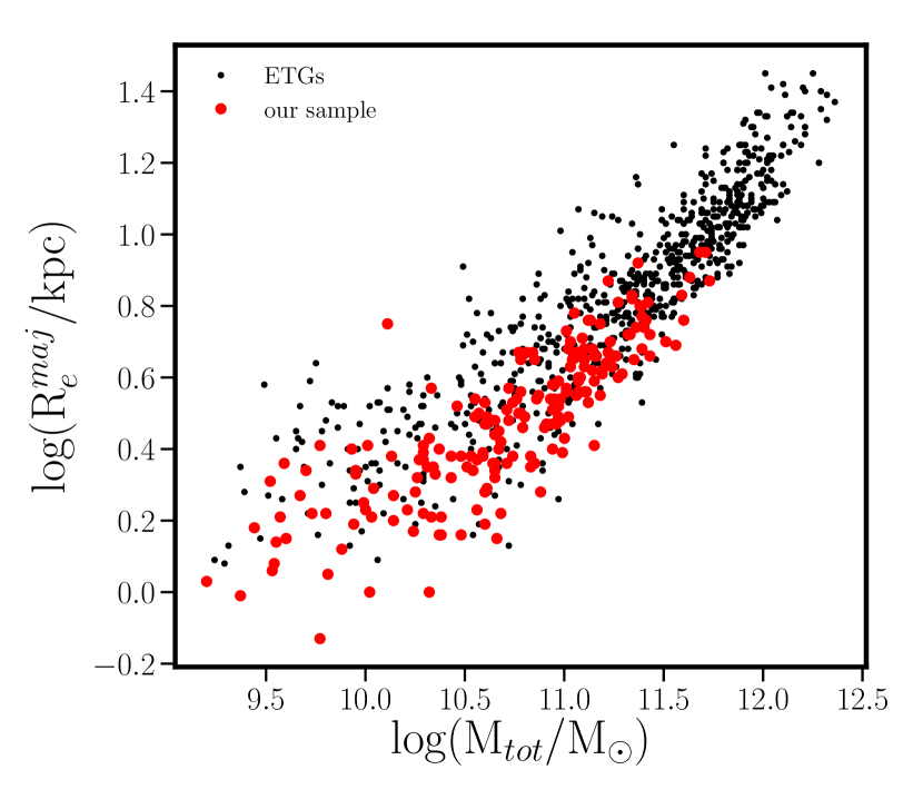
Figure 1 shows the mass-size distribution of our sample galaxies (red circles) comparing to the ETGs from the entire parent sample (black dots). The mass and size measurements are from L18. The masses are two times of the dynamical masses that are enclosed in 1R_e spheres. The sizes are the major axis of the half-light isophote (R${}_{e}^{maj}$).

Note that MaNGA applies a volume limited target selection. The more massive galaxies are from higher redshifts hence have lower S/N. Therefore our high-S/N selection criterion excludes the galaxies that are more massive than 10^11.8M_⊙. According to the studies from the literature, the global stellar population properties of the most massive and intermediate-mass ETGs have the same trends with galactic velocity dispersions (e.g., Thomas et al., 2005; McDermid et al., 2015). Thus the lack of ETGs at massive end should not affect our major results, at least for the relations between global stellar population parameters and $\sigma$.

We combine the light from the inner 1R${}_{e}^{maj}$ ellipse of our sample ETGs for the study of their global stellar population properties. The geometry calculation is based on the photometric position angle and ellipticity provided by Graham et al. (2018), together with the R${}_{e}^{maj}$ from L18. The blue histogram in Figure 2 illustrates the S/N distribution of these stacked spectra. The S/N shown in this figure is calculated by the best fitting spectra and the residuals. All the S/N is higher than 50, enough for our spectral fitting analysis (see §4.1).

When studying the stellar population gradients, we equally divide the galactic major axis in log space with the interval of 0.08 log(R${}_{e}^{maj}$), starting from 0.4 R${}_{e}^{maj}$. The central 0.4 R${}_{e}^{maj}$ ellipses are the innermost bins. Then we stack the spectra within each elliptical annulus.

We measure the one-dimension radial gradients within 1R${}_{e}^{maj}$ along the major axis. From Figure 2, the S/N of the radial bins at 1R${}_{e}^{maj}$ (red histogram) is acceptable for spectral fits (see §4.1). Beyond 1R${}_{e}^{maj}$, however, the S/N of the radial bins could be lower than 10, insufficient for an accurate spectral fitting analysis. Therefore we only calculate the gradients within 1R${}_{e}^{maj}$.

For the gradient calculations, we find the r-band luminosity weighted mean radius of each radial bin and fit the linear relation between log(R_mean/R${}_{e}^{maj}$) and [Z/H] or [$\alpha$/Fe]. We take the fitted slopes as radial gradients.

For each galaxy, we calculate the median S/N between 4800 and 5500 Å of the spectrum behind every spaxel in the DAP LOGCUB files. The signal and noise we adopt for this calculation are simply the flux and error provided by DAP. When doing stacking we only combine the spectra with S/N higher than 5. The DAP files provide the precise fits of emission lines (Westfall et al., 2019). We subtract the emission components before the fits.

For each stacked spectrum with emission line subtraction, we apply the pPXF spectral fitting programme to fit the r-band luminosity weighted stellar population parameters. The templates are made from the V15 models which are constructed on the BaSTI scaled-solar and $\alpha$-enhanced isochrones with a Salpeter IMF. pPXF produces the best fitted spectra by weighting templates.

The templates with [$\alpha$/Fe] = 0.0 and 0.4 correspond to the models with BaSTI scaled-solar and $\alpha$-enhanced isochrones respectively. At either [$\alpha$/Fe], V15 provides the templates with ages ranging from 0.03 to 14 Gyr with narrow steps and [Z/H] = [-2.27, -1.79, -1.49, -1.26, -0.96, -0.66, -0.35, -0.25, 0.06, 0.15, 0.26, 0.40]. We do not use these original templates for our fits. In [Z/H] dimension, we only choose the templates at [Z/H] = -1.49, -1.26, -0.96, -0.66, -0.35, 0.06, 0.26, and 0.40, in order to have similar intervals across the full range. At each [Z/H] and [$\alpha$/Fe], we linearly interpolate the templates in log(age) space from log(0.06 Gyr) to log(14 Gyr) to obtain 24 ages with equal interval.

V15 showed examples of the spectral fits of galactic spectra. They only fitted the spectra from 4800Å to 5500Å. In this work, we adopt the same wavelength range for our fits. The fit of each galactic spectrum iterates twice. In the first step, we apply 10-order both additive and multiplicative polynomials in order to obtain fine fits for bad pixel clipping. In the second step, we take the kinematic estimations from the first step as the initial guess, assume a reddening curve given by Calzetti et al. (2000) and do not apply any polynomials. The initial guess of E(B-V) is the value provided by the DAP map. In both steps, the templates are normalised by the r-band luminosity. The wavelength resolution of V15 templates is 2.5 Å. Although it is similar to that of the MaNGA spectra, during the fits we broaden it to the accurate MaNGA spectral resolution, which is a function of wavelength.

Before applying our spectral fits for the main results, we did test work with Lick index analysis (see §4.3). In our test work, the index analysis relates to two stellar population models, Thomas et al. (2011, hereafter TMJ11) and V15.

TMJ11 is constructed with a Salpeter IMF. It has the same spectral resolution as V15. TMJ11 provides the model grids of Lick indices that are produced from two sets of stellar evolutionary tracks. One is entirely based on Cassisi et al. (1997, hereafter C97), while the other is based on C97 at low metallicity but on Girardi et al. (2000, hereafter P00) at [Z/H]$\geqslant-$0.33. TMJ11 grids have age = [0.1, 0.2, 0.4, 0.6, 0.8, 1, 2, 3, 4, 5, 6, 7, 8, 9, 10, 11, 12, 13, 14, 15] Gyr, [Z/H] = [-2.25, -1.35, -0.33, 0.0, 0.35, 0.67], and [$\alpha$/Fe] = [-0.3, 0.0, 0.3, 0.5]. We keep their age dimensions and linearly interpolate the [Z/H] and [$\alpha$/Fe] dimensions across their full ranges with a step of 0.05 for our analysis.

For V15, we construct the model grids by measuring the Lick indices of their model templates. Still based on the V15 model templates that are constructed on BaSTI scaled-solar and $\alpha$-enhanced isochrones with a Salpeter IMF, we firstly measure the Lick indices of all the original spectral templates. Then, similar to TMJ11, we keep their age dimension and linearly interpolate the [Z/H] and [$\alpha$/Fe] dimensions across their full ranges with a step of 0.05.

DAP MAPS files provide the Lick index measurements of the spectrum behind each Voronoi binned spaxel at a 2.5 Å wavelength resolution, which is the same as the resolutions of TMJ11 and V15 model spectra. We calculate the mean indices by weighting the index maps within the stacking areas by the r-band luminosity. Then we choose certain indices to fit the three stellar population parameters by searching the minimum reduced $\chi^{2}$ solutions from the interpolated TMJ11 or V15 grids.

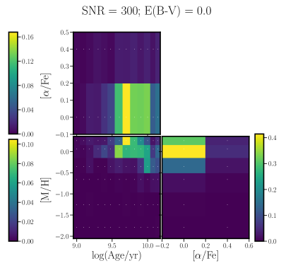
In order to test how the pPXF fits work on different stellar population compositions at a range of S/N, we test our methods on mock spectra first. We make the mock spectra with four stellar population compositions by weighting the V15 model templates which are constructed on the BaSTI scaled-solar or $\alpha$-enhanced isochrones with a Salpeter IMF. The left column in Figure 3 displays the projected weighting maps of these four stellar population compositions.

Two of them have one major component in each, mimicking single burst star formation histories. Both these two single major components are centred at log(age/Gyr) = log(6) and [Z/H] = 0.06 (the solar metallicity in V15 models). Their [$\alpha$/Fe] is centred at 0 and 0.4 respectively. Each component has an 1$\sigma$ Gaussian dispersion of ($\delta$(log(age/Gyr)), $\delta$([Z/H]), $\delta$([$\alpha$/Fe])) = (0.2, 0.3, 0.2).

Each of the other two compositions contains two major components. One composition mimics ETGs, which contains a compact “bulb" at a relatively old age, rich [Z/H], and high [$\alpha$/Fe] in the parameter space, plus a more extended younger component with lower [Z/H] and [$\alpha$/Fe]. These two components are centred at (log(age/Gyr), [Z/H], [$\alpha$/Fe]) = (log(10), 0.2, 0.3) and (log(3.5), -0.5, 0.1), with the 1$\sigma$ dispersion of ($\delta$(log(age/Gyr)), $\delta$([Z/H]), $\delta$([$\alpha$/Fe])) = (0.1, 0.15, 0.1) and (0.15, 0.3, 0.1), respectively.

The other composition is more similar to late-type galaxies. It contains a bulge component with a rapid metal enrichment history plus a disk component with a mild and extended star formation history. The mean (log(age/Gyr), [Z/H], [$\alpha$/Fe]) of the bulge and disk components are (log(10), -0.66, 0.25) and (log(2), 0.06, 0). The 1$\sigma$ dispersions ($\delta$(log(age/Gyr)), $\delta$([Z/H]), $\delta$([$\alpha$/Fe])) are (0.1, 0.5, 0.1) and (0.5, 0.3, 0.15) for the two components, respectively.

For each composition, we add constant noise and Calzetti et al. (2000) reddening curve to the combined mock spectra. The mean S/N we add are 5, 15, 30, 60, 100, 300, and 1000. The E(B-V) of our test spectra are either 0 or 0.3. Because the templates cannot be shrunk during the fitting procedures, we broaden our mock spectra to a velocity dispersion of 150 km/s.

The fitting method is the same as the second fit in each iteration for our MaNGA spectra. The only difference is that the templates used in the fits are the original model templates without interpolations, which are the same as the ones that make the mock spectra. Thus the difference between the parameters of the mock spectra and our fitting results will be purely driven by the fitting methods and the noise of the spectra. For each mock spectrum, after the simultaneous fits for both its stellar populations and kinematics, we fix the kinematic results as inputs and preform 500 bootstrapping realisations to estimate the scatter of the stellar population parameters.

We show the representative results of the weighting maps for the spectra at S/N = 5, 60, and 300 with E(B-V)=0 in Figure 3. Each row corresponds to one composition. From left to right, the first column displays the weighting maps of the mock spectra. The next three columns display the outputs at three S/N respectively. For all the four compositions, the results from S/N = 5 spectra do not show reasonable indications of age and [Z/H]. At S/N = 60, the fitting programmes may produce similar stellar population parameters to the input values, but fail in reconstructing the weighting maps. The input and output weighting maps become similar at S/N = 300, though not exactly the same. From the S/N distribution of our spectra (Figure 2), our fitting procedures will not be able to tell the accurate stellar components. Therefore we do not show the weighting maps from our scientific analysis in this paper.

Figure 4 shows the difference between the input and output of the stellar population parameters as functions of log(S/N). From (a) to (d), the magenta, green, and cyan colours represent log(age), [Z/H], and [$\alpha$/Fe], respectively. The circles and squares indicate the results from the spectra with E(B-V) = 0 and 0.3. In all cases, the differences converge to zero at S/N=10000. The differences at S/N$\sim$60 are below 0.05, which is acceptable for our study.

L18 applied pPXF to fit the ages and [Z/H] of MPL5 galaxies and provided the mean values within 1R_e. They used the similar methods but only searched the best fits from the two dimensional parameter space of age and [Z/H] with the use of Vazdekis et al. (2010, hereafter V10) templates. To check if our programmes work correctly, we apply our programmes on the entire MPL5 galaxies but replacing the V15 templates with V10. Then we compare our results with L18’s in Figure 5. Our parameter settings are the same as those in L18.

In Figure 5, the x and y-axis indicate the the age (left) and [Z/H] (right) measurements from and L18 and our work, respectively. Our results are in good agreement, indicating that our spectral fitting programmes are reliable. Note that L18 measured the age and [Z/H] of the Voronoi bins within 1R_e then averaged them respectively, while we estimate the parameters from the total light within 1R_e. However, the results should be basically the same with such small difference.

Zheng et al. (2019) studied the [$\alpha$/Fe]-$\sigma$ relation based on the entire MPL7 sample of 2997 galaxies. They did the analysis with the use of TMJ11 model and four indices of H_β, Mg$b$, Fe5270, and Fe5335. Although they included both star-forming and passive galaxies, the passive galaxies (H_β < 3) are significantly dominated in their massive sample and the star-forming and passive galaxies follow similar distributions of [$\alpha$/Fe] and $\sigma$ at low masses. Therefore we expect the [$\alpha$/Fe]-$\sigma$ relation shown in their work is similar to the relation fitted by the ETGs in their sample only.

To check the representativeness of our high-S/N sample, we repeat the analysis in Zheng et al. (2019) on the spectra stacked from the inner 1R${}_{e}^{maj}$ ellipses of our sample ETGs and compare our resulted [$\alpha$/Fe]-$\sigma$ relation with theirs. In Figure 6 we plot our [$\alpha$/Fe] measurements against log($\sigma_{e}$/km s^-1). The red and magenta dashed lines are the [$\alpha$/Fe]-log($\sigma$) relations fitted from our results of the entire and massive samples respectively. The cyan dot-dashed line is the [$\alpha$/Fe]-log($\sigma$) relation adopted from the Figure 17 in Zheng et al. (2019). The slopes of the red dashed line and the cyan dot-dashed line are 0.06 and 0.08, respectively. The small difference indicates that our sample is well representative. When limiting to the massive sample (log($\sigma_{e}$/km s^-1) > 1.9), the slope of the [$\alpha$/Fe]-log($\sigma$) relation is 0.22, agree with the results from the literature.

V15 showed another test with Lick index analysis. They estimated the “true [$\alpha$/Fe]" of 4671 nearby ETGs by fitting their [$\alpha$/Fe] and [Z/H] from three indices Mg$b$, [MgFe]’=$\sqrt{Mgb\times(0.72Fe5270+0.28Fe5335)}$, and Fe3=(Fe4383+Fe5270+Fe5335)/3 at fixed ages. The fixed ages were estimated by the spectral fitting method with V10 templates. Their results from the fits with V15 and TMJ11 models followed a relation as [$\alpha$/Fe]_V15=0.04+1.21[$\alpha$/Fe]_TMJ11. We apply the same analysis on the spectra stacked from the inner 1R${}_{e}^{maj}$ of our sample ETGs. Figure 7 shows the results. The relation that are fitted from our results is [$\alpha$/Fe]_V15=0.05+1.02[$\alpha$/Fe]_TMJ11 (red dashed line), consistent with the relation that V15 derived (yellow dot-dashed line) within uncertainties.

We stack the spectrum within the inner 1R${}_{e}^{maj}$ ellipse of each ETG in our sample and fit its [$\alpha$/Fe] by pPXF. In Figure 8 we show the spectral fits of two representative ETGs with different $\sigma_{e}$. On the top of each panel we label the related parameters, among which the S/N and three stellar population parameters are derived from the fits. In each panel, the top row displays the fits of the spectra over the entire wavelength range of 4800-5500Å. The middle and bottom rows are the zoom-in plots for Mg and Fe bands respectively. The black and green lines are the galactic spectra and the best fitting results. The cyan and magenta spectra are constructed by the model templates with the same weights in age and [Z/H] dimensions as the best fit’s. However, their [$\alpha$/Fe] are forced to be 0 or 0.4 respectively. The lower flat lines with fluctuations are the residuals from the fit. The colours correspond to the three colours of the fitting spectra. The grey horizontal line is the baseline for the residuals.

The blue bands illustrate the index bandpass of H_β. The magenta and cyan bands mark the $\alpha$-element and Fe indicators respectively. The three indices that indicate the $\alpha$-elements in this wavelength range are Mg₁, Mg₂, and Mg$b$. The Mg₂ and Mg$b$ indices are overlapped with each other. The four Fe tracers are Fe5015, Fe5270, Fe5335, and Fe5406. The grey bands are the regions which are excluded from our fits.

For both ETGs with different $\sigma_{e}$, the best fits match the spectra precisely. The cyan and magenta model spectra with different [$\alpha$/Fe] fail in fitting the Mg and Fe features. The magenta spectra with a higher [$\alpha$/Fe] have stronger Mg$b$ and weaker Fe absorption features. The cyan spectra show the offset in the opposite direction. These indicate that our spectral fitting programmes work well. Especially, they are able to tell the difference in [$\alpha$/Fe].

Particularly, the magenta and cyan spectra are above and below the green spectra at Mg₁ features respectively. It indicates that the V15 templates with higher [$\alpha$/Fe] have lower Mg₁ index values and vice versa. V15 mentioned such unusual behaviour of Mg₁. We have further discussions in Section 6.3.

Figure 9 presents our fitting results of [$\alpha$/Fe] as a function of log($\sigma_{e}$/km s^-1). The error bars show the 1$\sigma$ scatter from the bootstrapping fits with a 500 times realisation. Similar to the [$\alpha$/Fe]-$\sigma$ relations shown in Liu et al. (2016) and Zheng et al. (2019), the scatter of [$\alpha$/Fe] is relatively large at low masses. Unfortunately, we do not have enough low-mass ETGs for statistical analysis.

The red and magenta dashed lines are the fitted relations for our entire and massive (log($\sigma_{e}$/km s^-1) > 1.9) samples respectively. For reference, we plot the [$\alpha$/Fe]-log($\sigma$) relation from Zheng et al. (2019) as the cyan dot-dashed line (the same as the cyan dot-dashed line in Figure 6). The slopes of the red and magenta dashed lines are 0.01 and 0.03, respectively. The flatness of these relations indicates that the [$\alpha$/Fe] of ETGs from our analysis does not have significant dependence on galactic potential wells, even if limiting to the massive ETGs only.

At the same time, however, the results from our analysis with TMJ11 model support the classic positive [$\alpha$/Fe]-$\sigma$ relation of ETGs. From Section 4.3, the slopes of the TMJ11-based [$\alpha$/Fe]-log($\sigma_{e}$) relations of the same entire and massive samples (the red and magenta dashed lines in Figure 6) are 0.06 and 0.22 respectively. We will further discuss it in Section 6.

For reference, we show our measurements of age and [Z/H] as functions of log($\sigma_{e}$/km s^-1) in Figure 10. Both the log(age) and [Z/H] have positive correlations with log($\sigma_{e}$), in agreement with the results from the literature. The slopes of our log(age)-log($\sigma_{e}$) and [Z/H]-log($\sigma_{e}$) relations are 0.51 and 1.28. However, the former number is unreliable, for a significant fraction of our sample have their age estimations limited by the model’s upper boundary.

In Figure 11, we plot the V15 model grids in H_β-[MgFe]’ planes. The data points of our sample ETGs are colour coded according to their log($\sigma_{e}$/km s^-1). A significant fraction of our sample have their H_β lower than the model boundary, indicating that the oldest age in V15 models, 14 Gyr, is not enough for our oldest ETGs. As a result, the age measurements of these ETGs are limited by the model’s upper boundary, which are untrue.

Figure 12 presents the radial gradients of log(age), [Z/H], and [$\alpha$/Fe] within 1R${}_{e}^{maj}$ of our sample ETGs. The error bars show the 1$\sigma$ scatter from the Monte Carlo simulation with a 500 times realisation. The magenta symbols show the mean gradients and 1$\sigma$ scatter in every 0.2 interval of log($\sigma_{e}$/km s^-1) starting from 1.4. Their error bars show the scatter of the gradients within the log($\sigma_{e}$) bins. Figure 13 presents the log(age/Gyr), [Z/H], and [$\alpha$/Fe] profiles of the individual ETGs in different log($\sigma_{e}$) bins. The magenta dots and error bars illustrate the mean radii, mean log(age/Gyr), [Z/H], or [$\alpha$/Fe], and the mean 1$\sigma$ uncertainties of them within the radial bins. In both figures, the grey symbols in the top panel indicate the ETGs which have ages reaching the model boundary in more than one radial bins, and they are not taken into account in the mean calculation.

On average, the age and [Z/H] gradients have similar trends with log($\sigma_{e}$), but the age profiles are much flatter at each $\sigma_{e}$. The [Z/H] gradients are positive at low $\sigma_{e}$. They gradually decrease to negative in the high-mass range. The [$\alpha$/Fe] gradients are flat when log($\sigma_{e}$/km s^-1) is below 2.1. This agrees with the previous results, e.g., Mehlert et al. (2003); Kuntschner (2004); Greene et al. (2015); Alton et al. (2018); Parikh et al. (2019). At higher $\sigma_{e}$, it slightly turns to positive. Goddard et al. (2017) measured the age and metallicity gradients of the ETGs from the MaNGA MPL4 sample. They employed the FIREFLY spectral fitting code (Maraston & Strömbäck, 2011) to analysis the stellar populations and divided the space by Voronoi binning method. Though their results of age gradients are generally zero, they are consistent with ours within error bars. Their metallicity gradients are similar to ours, which are, on average, positive at low masses, and gradually decrease to zero and then negative as the increase of galactic masses. Based on the CALIFA data, Martín-Navarro et al. (2018) stacked 45 massive ETGs with $\sigma_{e}$ > 150 km/s in three $\sigma_{e}$ bins and made their stellar population radial profiles within 1R_e. Their [Z/H] gradients are negative, and the age and [$\alpha$/Fe] gradients are close to zero. These are all in agreement with our results.

These results indicate that massive ETGs have higher metallicity, slightly older ages and lower [$\alpha$/Fe] in galactic central regions. The differences between central and outer regions get larger as galactic mass increases. For the flat age gradients, probably because in galactic centres the star formation processes start earlier and last longer, and the balance of old and young stars makes the mean stellar ages in galactic centres similar to the outer regions. The slightly more old or young stars in central regions would make the gradients little negative or positive.

Regarding to the [Z/H] and [$\alpha$/Fe] gradients, in massive ETGs, the reasons might be that they have deeper gravitational potential wells in the centre therefore have higher gas content to support more extended star formation activities than in outskirts. In intermediate-mass galaxies, though the central regions still have more intense star formation activities than outside, the metal enriched gas in the centres are easier to be blown out and fall into outer regions comparing to the most massive galaxies. Thus less massive ETGs have flatter profiles.

In the low-mass range, while the [$\alpha$/Fe] profiles are flat, a significant fraction of galaxies have positive metallicity gradients, indicating a lower metallicity in galactic centres. A possible scenario is that the star formation activities of low-mass galaxies do not vary too much from centre to outside. At the same time, galactic central regions have more infall gas with relatively low metallicity. When the central metal enrichment cannot overcome the metallicity dilution caused by gas infall, there will be a positive metallicity gradient.

A caveat is that the uncertainty of these radial gradient estimations cannot be neglected, especially for ages and [$\alpha$/Fe]. From Figure 11, the resolution of age estimations is low when it is older than 7 Gyr. Thus the age radial profiles could significantly change after considering the uncertainties at old ages. In Section 6.3, we demonstrate that V15 models might underestimate the [$\alpha$/Fe] of some massive ETGs. Such underestimation might flatten the intrinsically positive [$\alpha$/Fe]-$\sigma$ relation and make the [$\alpha$/Fe] distribution flat in Figure 9. At the same time, it could also flatten the [$\alpha$/Fe] radial profiles.

Using pPXF, our spectral fitting method looks for the best weightings of the templates with different stellar population parameters. Essentially, it looks for the best combinations of different stellar population components. The results are the composite stellar population (CSP) parameters. However, our index analysis works in a different way. It searches the best matched single-equivalent stellar population (SSP) parameters from the model grids.

To investigate the difference between CSP and SSP results, we interpolate the V15 templates according to the ages, [Z/H], and [$\alpha$/Fe] in the interpolated V15 model grid of Lick indices we introduce in Section 3.3. Then we apply pPXF to fit our galactic spectra that are stacked from the inner 1R${}_{e}^{maj}$ ellipses with a single interpolated template at one time. Thus we are searching the best fitting SSP templates. The parameter settings and the wavelength range for our fits are the same as what we adopt for the analysis in Section 5.1.

Figure 14 presents how the [$\alpha$/Fe] measurements change after we switch the spectral fits into SSP mode. The y-axis is the difference between the SSP results and our CSP results which Figure 9 shows. From left to right, the x-axis indicates log($\sigma_{e}$/km s^-1), log(age/Gyr), and [Z/H]. The [Z/H] is derived from the same spectral fitting analysis for our [$\alpha$/Fe] estimations. In Section 5.1 we mention that a significant fraction of our sample have their age estimations reach the model boundary of 14 Gyr. To avoid this problem, the age measurements are from the spectral fits with V10 templates. The yellow horizontal dashed lines mark the zero difference.

In the high-mass range, the differences are relatively small (below 0.1 dex). At low $\sigma$, the SSP results are systematically higher. These changes do not change our result of a flat [$\alpha$/Fe]-log($\sigma_{e}$) relation of ETGs, especially at massive end. The slopes of the SSP based [$\alpha$/Fe]-log($\sigma_{e}$) relations for the entire and massive samples are 0.0 and 0.07.

The differences correlate with [Z/H] best. Below [Z/H]$=-$0.5, the difference becomes larger at lower [Z/H]. It is probably due to the degeneracy between low [Z/H] and high [$\alpha$/Fe], and the CSP fits have an advantage in breaking the degeneracy. Above [Z/H]$=-$0.4, the [$\alpha$/Fe] differences show a positive correlation with [Z/H]. However, this is because of the inclusion of the wavelength ranges for Mg₁ and Fe5015.

According to the Figure 13 in V15, Mg₁, which is traditionally regarded as an indicator of $\alpha$ elements, has unusual behaviours. When the ages are older than 1 Gyr, at a same [Z/H], the V15 templates with higher [$\alpha$/Fe] have lower Mg₁ index values. The reason is possibly that Mg₁ is more sensitive to C than Mg. Besides, because Fe5015 is sensitive to both Fe and Ti, an $\alpha$ element, it shows less sensitivity to the change of $\alpha$ element abundance in the models comparing to other Fe indicators.

We mask the wavelength ranges of Mg₁ and Fe5015 and repeat both the SSP and CSP fits for our sample ETGs. Figure 15 is similar to Figure 14 but the y-axis is the difference between the SSP-[$\alpha$/Fe] and CSP-[$\alpha$/Fe] that are measured under the masks. In this figure, the difference is still anti-correlated with [Z/H] at low [Z/H], but the dependence with [Z/H] disappears above [Z/H]$=-$0.5.

Another key difference between our spectral fits and index analysis is that they take information from different spectral features. While the former takes into account the flux at every wavelength, the latter only makes use of the most prominent features within the wavelength range. In this section we examine how much difference the non-prominent features would make in the [$\alpha$/Fe] measurement.

The wavelength range for our spectral fits (4800-5500Å) covers 8 Lick indices: H_β, Fe5015, Mg₁, Mg₂, Mg$b$, Fe5270, Fe5335, and Fe5406. We apply the same spectral fitting methods as we do for the main scientific results on the spectra stacked from the inner 1R${}_{e}^{maj}$ ellipses of our sample ETGs, but limiting the wavelength range to the bands of these Lick indices only. Then we compare the resulted [$\alpha$/Fe] to our main results. Similar to Figure 14, Figure 16 shows the difference as functions of log($\sigma_{e}$/km s^-1), log(age/Gyr), and [Z/H]. For all of our ETGs, the [$\alpha$/Fe] measured from two wavelength ranges are consistent with each other within the uncertainties. It indicates that over 4800-5500Å, the non-prominent spectral features do not make significant difference in stellar population analysis.

In Section 6.1 we mention that Mg₁ has higher values in the scaled-solar models than in the $\alpha$-enhanced models. It is contrary to the behaviours of Mg₁ in other stellar population models (e.g., TMJ11). In Figure 17 we compare the model grids of V15 and TMJ11. We plot the grids of these two models in black and cyan respectively. The upper panels display the grids in Mg₁-$<$Fe$>$ planes. The [Z/H] and [$\alpha$/Fe] values are labeled beside the corresponding isolines. We colour code the data points according to the log($\sigma_{e}$/km s^-1) of our sample ETGs. At each [Z/H], while the Mg₁ index has a higher value at a higher [$\alpha$/Fe] in TMJ11 model, it behaves inversely in V15 models. In the lower panels, we replace the Mg₁ with Mg$b$ for y-axis. In this case, in both models, the Mg$b$ index has higher values at higher [$\alpha$/Fe]. The different behaviour of Mg₁ may be due to the different treatment of C in two models. From the Figure 1 in Johansson et al. (2012), while Mg$b$ is mostly sensitive to Mg abundance, Mg₁ is much more sensitive to the abundance of C comparing to Mg.

It is possible that Mg₁ plays a role in shaping the [$\alpha$/Fe]-$\sigma$ relation. Therefore we compare the results from the fits with and without Mg₁ to examine the role of Mg₁. In Section 6.2 we apply the spectral fits with the wavelength coverage of only the 8 Lick indices within 4800-5500Å. Here we exclude the Mg₁ index and repeat the fits on the same data we apply in Section 6.2.

We compare the [$\alpha$/Fe] results from the fits over the bands of 7 and 8 Lick indices. Figure 18 shows the differences. While including Mg₁ or not does not change the [$\alpha$/Fe] measurements at log($\sigma_{e}$/km s^-1)$<$2.1, the difference increases with $\sigma$ at the massive end. At super solar [Z/H]  log(age/Gyr)>0.7, or log($\sigma_{e}$/km s^-1)$>$2.1, the differences have slightly tighter correlation with [Z/H] or log(age) than with log($\sigma_{e}$). It implies that the Mg₁-driven difference is related to [Z/H]. According to V15, the $\alpha$-enhanced models at high metallicity incorporate theoretical differential spectral response to switch from the abundance pattern of the Milky Way to the desired enhancement. However, the computation of very cool star spectra, which contribute to the molecular bands like MgH is difficult, making these features less reliable for the analysis performed here. We suggest avoiding this rather wide index, which covers 471Å, as it might suffer from other effects such as flux-calibration issues.

Such offset of the [$\alpha$/Fe] measurements at high-[Z/H] and massive ends significantly steepens the [$\alpha$/Fe]-$\sigma$ relation. In Figure 19 we plot the [$\alpha$/Fe] measured from the spectral fits over the 7 indices against log($\sigma_{e}$/km s^-1). The red and magenta dashed lines are the relations fitted from the entire and massive samples, with the slopes of 0.1 and 0.13 respectively. The yellow dot-dashed line is the relation from our main results (the magenta dashed line in Figure 9), plotted for reference.

In Figure 20, we show more direct comparisons. In Section 4.3, we mention the Lick index approach which V15 suggested. They estimated the “true [$\alpha$/Fe]" by fitting [$\alpha$/Fe] and [Z/H] with three indices Mg$b$, [MgFe]’=$\sqrt{Mgb\times(0.72Fe5270+0.28Fe5335)}$, and Fe3=(Fe4383+Fe5270+Fe5335)/3 at the fixed ages which were derived from the the spectral fits with V10 templates. We have repeated such analysis with both V15 and TMJ11 models on our sample. In Figure 7 we compare the [$\alpha$/Fe] results measured from two models and the correlation is in agreement with V15’s. In Figure 20, we plot these [$\alpha$/Fe] results against log($\sigma_{e}$/km s^-1) in the left column. The upper and lower panels indicate the results from V15 and TMJ11 models respectively. The magenta dashed lines illustrate the linear relations that are fitted from the massive sample. In each panel, we label the slope of the relation in the upper left corner. The [$\alpha$/Fe] fitted from both models has positive correlation with log($\sigma_{e}$) in the massive ranges, but the scatter is larger when using V15 models.

At the same time, we fit the [$\alpha$/Fe] using the same methods but including Mg₁ in our fits in addition to those three indices. We show the results correspondingly in the right column. The inclusion of Mg₁ flattens the classic positive relation when using V15 models. By contrast, using TMJ11 model, the positive [$\alpha$/Fe]-$\sigma$ relation of massive ETGs still holds after the inclusion of Mg₁. The slope becomes even steeper. This is because from Figure 17, our massive sample locate in the positions with higher [$\alpha$/Fe] in Mg₁-$<$Fe$>$ planes than in Mg$b$-$<$Fe$>$ planes. The different relations between log($\sigma_{e}$) and the [$\alpha$/Fe] fitted by different models with or without the inclusion of Mg₁ indicate that V15 models have difficulties in covering the observations in Mg₁.

As mentioned in the introduction, all the previous stellar population analysis with other stellar population models show positive correlations between the global [$\alpha$/Fe] and $\sigma$ among massive ETGs. Although some simulations can produce the positive slopes (e.g., Arrigoni et al., 2010; Yates et al., 2013; Segers et al., 2016; Vincenzo et al., 2018), they all include special mechanisms, e.g., more top-heavy IMFs, different supernova properties, and AGN feedback. None of these mechanisms has been supported by robust evidence from observations.

A potential reason for the discrepancy is that simulations and observations use different $\alpha$ element indicators. In simulations the most common [$\alpha$/Fe] indicator is [O/Fe]. Comparing to [Mg/Fe] and [Si/Fe], the [O/Fe] distribution of the Milky Way stars matches the theoretical predictions better (Matteucci & Greggio, 1986). However, comparing to Mg, it is more difficult to estimate the stellar O abundance using relatively low resolution spectra of the integral extragalactic light. Therefore in most stellar population analysis, the $\alpha$ elements are traced by Mg.

In most previous studies, the adopted indicator of $\alpha$ elements is Mg$b$ index. From our analysis, the inclusion of Mg₁ makes difference in the [$\alpha$/Fe] measurements of ETGs with super-solar [Z/H]. On one hand, according to Section 6.3, we suggest that it is a consequence of the self-inconsistency of V15 models. On the other hand, it indicates that we cannot rule out the probability that the [$\alpha$/Fe] of massive ETGs is not correlated with their $\sigma$. In other words, though the probability is low, the galaxies with deeper potential wells might not have more intense early star formation processes, different IMFs, or special supernova properties.

References

- Alton et al. (2018) Alton P. D., Smith R. J., Lucey J. R., 2018, MNRAS, 478, 4464
- Arrigoni et al. (2010) Arrigoni M., Trager S. C., Somerville R. S., Gibson B. K., 2010, MNRAS, 402, 173
- Bundy et al. (2015) Bundy K., et al., 2015, ApJ, 798, 7
- Calzetti et al. (2000) Calzetti D., Armus L., Bohlin R. C., Kinney A. L., Koornneef J., Storchi-Bergmann T., 2000, ApJ, 533, 682
- Cappellari (2016) Cappellari M., 2016, ARA&A, 54, 597
- Cappellari (2017) Cappellari M., 2017, MNRAS, 466, 798
- Cappellari & Copin (2003) Cappellari M., Copin Y., 2003, MNRAS, 342, 345
- Cappellari & Emsellem (2004) Cappellari M., Emsellem E., 2004, PASP, 116, 138
- Cassisi et al. (1997) Cassisi S., Castellani M., Castellani V., 1997, A&A, 317, 108
- Cid Fernandes et al. (2005) Cid Fernandes R., Mateus A., Sodré L., Stasińska G., Gomes J. M., 2005, MNRAS, 358, 363
- Conroy et al. (2018) Conroy C., Villaume A., van Dokkum P. G., Lind K., 2018, ApJ, 854, 139
- Ferreras & Silk (2003) Ferreras I., Silk J., 2003, MNRAS, 344, 455
- Ge et al. (2018) Ge J., Yan R., Cappellari M., Mao S., Li H., Lu Y., 2018, MNRAS, 478, 2633
- Girardi et al. (2000) Girardi L., Bressan A., Bertelli G., Chiosi C., 2000, A&AS, 141, 371
- Goddard et al. (2017) Goddard D., et al., 2017, MNRAS, 466, 4731
- González Delgado et al. (2015) González Delgado R. M., et al., 2015, A&A, 581, A103
- Graham et al. (2018) Graham M. T., et al., 2018, MNRAS, 477, 4711
- Graves & Schiavon (2008) Graves G. J., Schiavon R. P., 2008, ApJS, 177, 446
- Greene et al. (2015) Greene J. E., Janish R., Ma C.-P., McConnell N. J., Blakeslee J. P., Thomas J., Murphy J. D., 2015, ApJ, 807, 11
- Johansson et al. (2012) Johansson J., Thomas D., Maraston C., 2012, MNRAS, 421, 1908
- Kuntschner (2004) Kuntschner H., 2004, A&A, 426, 737
- Kuntschner et al. (2010) Kuntschner H., et al., 2010, MNRAS, 408, 97
- Law et al. (2016) Law D. R., et al., 2016, AJ, 152, 83
- Li et al. (2018) Li H., et al., 2018, MNRAS, 476, 1765
- Lintott et al. (2008) Lintott C. J., et al., 2008, MNRAS, 389, 1179
- Lintott et al. (2011) Lintott C., et al., 2011, MNRAS, 410, 166
- Liu et al. (2016) Liu Y., Ho L. C., Peng E., 2016, ApJ, 829, L26
- Maoz et al. (2010) Maoz D., Sharon K., Gal-Yam A., 2010, ApJ, 722, 1879
- Maraston & Strömbäck (2011) Maraston C., Strömbäck G., 2011, MNRAS, 418, 2785
- Martín-Navarro et al. (2018) Martín-Navarro I., Vazdekis A., Falcón-Barroso J., La Barbera F., Yıldırım A., van de Ven G., 2018, MNRAS, 475, 3700
- Matteucci & Greggio (1986) Matteucci F., Greggio L., 1986, A&A, 154, 279
- Matteucci & Tornambe (1987) Matteucci F., Tornambe A., 1987, A&A, 185, 51
- McDermid et al. (2015) McDermid R. M., et al., 2015, MNRAS, 448, 3484
- Mehlert et al. (2003) Mehlert D., Thomas D., Saglia R. P., Bender R., Wegner G., 2003, A&A, 407, 423
- Monachesi et al. (2019) Monachesi A., et al., 2019, MNRAS, 485, 2589
- Ogando et al. (2005) Ogando R. L. C., Maia M. A. G., Chiappini C., Pellegrini P. S., Schiavon R. P., da Costa L. N., 2005, ApJ, 632, L61
- Okamoto et al. (2017) Okamoto T., Nagashima M., Lacey C. G., Frenk C. S., 2017, MNRAS, 464, 4866
- Oliva-Altamirano et al. (2015) Oliva-Altamirano P., Brough S., Jimmy Tran K.-V., Couch W. J., McDermid R. M., Lidman C., von der Linden A., Sharp R., 2015, MNRAS, 449, 3347
- Parikh et al. (2019) Parikh T., et al., 2019, MNRAS, 483, 3420
- Sánchez-Blázquez et al. (2007) Sánchez-Blázquez P., Forbes D. A., Strader J., Brodie J., Proctor R., 2007, MNRAS, 377, 759
- Segers et al. (2016) Segers M. C., Schaye J., Bower R. G., Crain R. A., Schaller M., Theuns T., 2016, MNRAS, 461, L102
- Thomas et al. (1999) Thomas D., Greggio L., Bender R., 1999, MNRAS, 302, 537
- Thomas et al. (2003) Thomas D., Maraston C., Bender R., 2003, MNRAS, 339, 897
- Thomas et al. (2005) Thomas D., Maraston C., Bender R., Mendes de Oliveira C., 2005, ApJ, 621, 673
- Thomas et al. (2011) Thomas D., Maraston C., Johansson J., 2011, MNRAS, 412, 2183
- Tortora et al. (2011) Tortora C., Romeo A. D., Napolitano N. R., Antonuccio-Delogu V., Meza A., Sommer-Larsen J., Capaccioli M., 2011, MNRAS, 411, 627
- Vazdekis et al. (2010) Vazdekis A., Sánchez-Blázquez P., Falcón-Barroso J., Cenarro A. J., Beasley M. A., Cardiel N., Gorgas J., Peletier R. F., 2010, MNRAS, 404, 1639
- Vazdekis et al. (2015) Vazdekis A., et al., 2015, MNRAS, 449, 1177
- Vincenzo et al. (2018) Vincenzo F., Kobayashi C., Taylor P., 2018, MNRAS, 480, L38
- Westfall et al. (2019) Westfall K. B., et al., 2019, arXiv e-prints,
- Wilkinson et al. (2015) Wilkinson D. M., et al., 2015, MNRAS, 449, 328
- Wilkinson et al. (2017) Wilkinson D. M., Maraston C., Goddard D., Thomas D., Parikh T., 2017, MNRAS, 472, 4297
- Worthey et al. (1994) Worthey G., Faber S. M., Gonzalez J. J., Burstein D., 1994, ApJS, 94, 687
- Yates et al. (2013) Yates R. M., Henriques B., Thomas P. A., Kauffmann G., Johansson J., White S. D. M., 2013, MNRAS, 435, 3500
- Zheng et al. (2019) Zheng Z., et al., 2019, ApJ, 873, 63