SCOUTER: Slot Attention-based Classifier for Explainable Image Recognition
Abstract
Explainable artificial intelligence has been gaining attention in the past few years. However, most existing methods are based on gradients or intermediate features, which are not directly involved in the decision-making process of the classifier. In this paper, we propose a slot attention-based classifier called SCOUTER for transparent yet accurate classification. Two major differences from other attention-based methods include: (a) SCOUTER’s explanation is involved in the final confidence for each category, offering more intuitive interpretation, and (b) all the categories have their corresponding positive or negative explanation, which tells “why the image is of a certain category” or “why the image is not of a certain category.” We design a new loss tailored for SCOUTER that controls the model’s behavior to switch between positive and negative explanations, as well as the size of explanatory regions. Experimental results show that SCOUTER can give better visual explanations in terms of various metrics while keeping good accuracy on small and medium-sized datasets. Code is available111https://github.com/wbw520/scouter.
1 Introduction
It is of great significance to know how deep models make predictions, especially for the fields like medical diagnosis, where potential risks exist when black-box models are adopted. Explainable artificial intelligence (XAI), which can give a close look into models’ inference process, therefore has gained lots of attention.
The most popular paradigm in XAI is attributive explanation, which gives the contribution of pixels or regions to the final prediction [31, 7, 28, 30]. One natural question that arises here is how these regions contribute to the decision. For a better view of this, let denotes a fully-connected (FC) classifier for category , where and are trainable vector and scalar, respectively. Training this classifier may be interpreted as a process to find from the training samples a combination of discriminative patterns with corresponding weight , i.e.,
| (1) |
In general, these patterns can include positive and negative ones. Given of an image of , a positive pattern gives . A negative pattern, in contrast, gives for of any category other than , which means that the presence of pattern described by is a support of not being category . Therefore, set of all (linearly independent) patterns for can be the union of sets and of all positive and negative patterns.
Differentiation of positive/negative patterns gives useful information on the decision. Figure LABEL:fig_story(top) shows an MNIST image for example. One of positive patterns that makes the image being 7 can be the acute angle formed by white line segments that appears around the top-right corner, as in the second image. Meanwhile, the sixth image shows that the presence of the horizontal line is the support not being 1. A more practical application [2] in medical image analysis also points out the importance of visualizing positive/negative patterns. Nevertheless of the obvious benefit, recent mainstream methods like [49, 31, 27, 10] have not extensively studied this differentiation.
Positive and negative patterns lead to two interesting questions: (i) Can we provide positive explanation and negative explanation that visually show support regions in the image that correspond to positive and negative patterns? (ii) As the combination of patterns to be learned is rather arbitrary and any combination is possible as long as it is discriminative; can we provide preference on the combination in order to leverage prior knowledge on the task in training?
In this paper, we re-formulate explainable AI with an explainable classifier, coined SCOUTER (Slot-based COnfigUrable and Transparent classifiER), which tries to find either positive or negative patterns in images. This approach is similar to the attention-based approach (e.g. [21, 40]) rather than the post-hoc approaches [49, 31, 30]. Our newly proposed explainable slot attention (xSlot) module is the main building block of SCOUTER. This module is built on top of the recently-emerged slot attention [23], which offers an object-centric approach for image representation. The xSlot module identifies the spatial support of either positive or negative patterns for each category in the image, which is directly used as the confidence value of that category; the commonly-used FC classifier is no longer necessary. The xSlot module can also be used to visualize the support as shown in Fig. LABEL:fig_story. SCOUTER is also characterized by its configurability over patterns to be learned, i.e., the choice of positive or negative pattern and the desirable size of the pattern, which can incorporate the prior knowledge on the task. The controllable size of explanation can be beneficial for some applications, e.g., disease diagnosis in medicine, defect recognition in manufacturing, etc.
Contribution
Our transparent classifier, SCOUTER, explicitly models positive and negative patterns with a dedicated loss, allowing to set preference over the spatial size of patterns to be learned. We experimentally show that SCOUTER successfully learns both positive and negative patterns and visualize their support in the given image as the explanation, achieving state-of-the-art results in several commonly-used metrics like IAUC/DAUC [27]. Our case study in medicine also highlights the importance of both types of explanations as well as controlling the area size of explanatory regions.
2 Related Work
2.1 Explainable AI
There are mainly three XAI paradigms [43], i.e. post-hoc, intrinsic, and distillation. The post-hoc paradigm usually provides a heat map highlighting important regions for the decision (e.g. [31, 30]). The heat map is computed besides the forward path of the model. The intrinsic paradigm explores the important piece of information within the forward path of the model, e.g., as attention maps (e.g. [21, 40, 24, 42]). Distillation methods are built upon model distillation [16]. The basic idea is to use an inherently transparent model to mimic the behaviors of a black-box model (e.g. [48, 29]).
The post-hoc paradigm has been extensively studied among them. The most popular type of methods is based on channel activation or back-propagation, including CAM [49], GradCAM [31], DeepLIFT [32], and their extensions [3, 25, 36, 35, 7]. Another type of method is perturbation-based, including Occlusion [45], RISE [27], meaningful perturbations [11], real-time saliency [5], extremal perturbations [10], I-GOS [28], IBA [30], etc. These methods basically give attributive explanation, which visualizes support regions of learned patterns for each category in the set of all possible categories . This visualization can be done by finding regions in feature maps or the input image that give large impact on the score . By definition, attributive explanation is the same as our positive explanation.
Some of the methods for attributive explanation thus can be extended to provide negative explanations by negating the sign of the score, feature maps, or gradients. It should be noted that the interpretation of visual explanation by gradient-based methods [31, 3, 25] may not be straightforward because of linearization of for the given image; and thus the resulting visualization may not highlight the support regions for negative patterns. GradCAM [31] refers to its negative variant as counterfactual explanation that gives regions that can change the decision, emphasizing how it should be interpreted.
Discriminant explanation is a new type of XAI in the post-hoc paradigm, which appeared in [38] to show “why image belongs to category rather than .” This can be interpreted using set of all possible positive patterns for and set of all possible negative patterns for : It try to spot a (combination of) discriminative pattern that is in the intersection . Due to the unavailability of negative patterns, the method [38] first finds (a combination of) positive patterns and uses the complementary of the region containing the positive patterns as a proxy of negative patterns. Goyal et al. gives another line of counterfactual explanation in [13]. Given two images of categories and , they find the region in the image of , of which replacement to a certain region in the image of changes the prediction from to . This can be also implemented using discriminant explanation.
SCOUTER computes a heat map to spot regions important for the decision in the forward path, so it falls into the intrinsic paradigm. Together with the dedicated loss, it can directly identify positive and negative patterns with control over the size of patterns.
2.2 Self-attention in Computer Vision
Self-attention is first introduced in the Transformers [34], in which self-attention layers scan through the input elements one by one and update them using the aggregation over the whole input. Initially, self-attention is used in place of recurrent neural networks for sequential data, e.g., natural language processing [8]. Recently, self-attention is adopted to the computer vision field, e.g., Image Transformer [26], Axial-DeepLab [37], DEtection TRansformer (DETR) [1], Image Generative Pre-trained Transformer (Image GPT) [4], etc. Slot attention [23] is also based on this mechanism to extract object-centric features from images (there are some other works [15, 12] using the concept of slot); however, the original slot attention is tested only on some synthetic image datasets. SCOUTER is based on slot attention but is designed to be an explainable classifier applicable to natural images.


3 SCOUTER
Given an image , the objective of a classification model is to find its most probable category in category set . This can be done by first extracting features using a backbone network . is then mapped into a score vector , representing the confidence values, using FC layers and softmax as the classifier. However, such FC classifiers can learn an arbitrary (nonlinear) transformation and thus can be black-box.
We replace such an FC classifier with our SCOUTER (Fig. 1(a)), consisting of the xSlot attention module, which produces the confidence for each category given features . The whole network, including the backbone, is trained with the SCOUTER loss, which provides control over the size of support regions and switching between positive and negative explanations.
3.1 xSlot Attention
In the original slot attention mechanism [23], a slot is a representation of a local region aggregated based on the attention over the feature maps. A single slot attention module with multiple slots is attached on top of the backbone network . Each slot produces its own feature as output. This configuration is handy when there are multiple objects of interest. This idea can be transferred to spot the supports in the input image that leads to a certain decision.
The main building block of SCOUTER is the xSlot attention module, which is a variant of the slot attention module tailored for SCOUTER. Each slot of the xSlot attention module is associated with a category and gives the confidence that the input image falls into the category. With the slot attention mechanism, the slot for category is required to find support in the image that directly correlates to .
Given feature , the xSlot attention module updates slot for times, where represents the slot after updates and is the category associated to this slot. The slot is initialized with random weights, i.e.,
| (2) |
where and are the mean and variance of a Gaussian, and is the size of the weight vector. We denote the slots for all categories by .
The slot is updated using and feature . Firstly, goes through a convolutional layer to reduce the number of channels and the ReLU nonlinearity as , with ’s spatial dimensions being flattened (). is augmented by adding the position embedding to take the spatial information into account, following [34, 1], i.e. , where PE is the position embedding. We then use two multilayer perceptrons (MLPs) and , each of which has three FC layers and the ReLU nonlinearity between them. This design is for giving more flexibility in the computation of query and key in the self-attention mechanism. Using
| (3) |
we obtain the dot-product attention using sigmoid as
| (4) |
The attention is used to compute the weighted sum of features in the spatial dimensions by
| (5) |
and slot is eventually updated through a gated recurrent unit (GRU) as
| (6) |
taking and as input and hidden state, respectively. Following the original slot attention module, we update the slot for times.
The output of the xSlot attention module is the sum of all elements for category in , which is a function of . Formally, the output of xSlot Attention module is:
| (7) |
where is the column vector with all elements being 1.
From Eqs. (5) and (7), we have , where is a reduction of and is a class-agnostic map. The -th row of can then be viewed as spatial weights over map to spot where the support regions for category is222 can be viewed as a single map that includes a mixture of supports for all categories.. In order for visualizing the support regions, we reshape and resize each row of to the input image size.
Note that in the original slot attention module, a linear transformation is applied to the features, i.e., , which is then weighted using Eq. (5). However, the xSlot attention module omits this transformation as it already has a sufficient number of learnable parameters in , , GRU, etc., and thus the flexibility. Also, the confidences, given by Eq. (7), are typically computed by an FC layer, while SCOUTER just sums up the output of xSlot attention module, which is actually the presence of learned supports for each category. This simplicity is essential for a transparent classifier as discussed in Section 3.3.
3.2 SCOUTER Loss
The whole model, including the backbone network, can be trained by simply applying softmax to xSlot and minimizing cross-entropy loss . However, there is a phenomenon that, in some cases, the model prefers attending to a broad area (e.g., a slot covers a combination of several supports that occupy large areas in the image) depending on the content of the image. As argued in Section 1, it can be beneficial to have control over the area of support regions to constrain the coverage of a single slot.
Therefore, we design the SCOUTER loss to limit the area of support regions. The SCOUTER loss is defined by
| (8) |
where is the area loss, is a hyper-parameter to adjust the importance of the area loss. The area loss is defined by
| (9) |
which simply sums up all the elements in . With larger , SCOUTER attends smaller regions by selecting fewer and smaller supports. On the contrary, it prefers a larger area with smaller .
3.3 Switching Positive and Negative Explanation
The model with the SCOUTER loss in Eq. (8) can only provide positive explanation since larger elements in means the prediction is made based on the corresponding features. We introduce a hyper-parameter in Eq. (7), i.e.,
| (10) |
where . This hyper-parameter configures the xSlot attention module to learn to find either positive or negative supports.
With the softmax cross-entropy loss, the model learns to give the largest confidence corresponding to ground-truth (GT) category and a smaller value to wrong category . For , all elements given by is non-negative since both and are non-negative and thus is. For arbitrary non-negative , thanks to simple reduction in Eq. (7), larger can be produced only when some elements in , the row vector in corresponding to , is close to 1, whereas a smaller is given when all elements in are close to 0. Therefore, by setting to , the model learns to find the positive supports among the images of the GT category. The visualization of thus serves as positive explanation, as in Fig. LABEL:fig_story (left).
On the contrary, for , all elements in are negative and thus the prediction by Eq. (10) gives close to 0 for correct category and smaller for non-GT category . To make close to 0, all elements in must be close to 0, and a smaller is given when has some elements close to 1. For this, the model learns to find the negative supports that do not appear in the images of the GT category. As a result, can be used as negative explanation, as shown in Fig. LABEL:fig_story (right).
4 Experiments
4.1 Experimental Setup
We chose to use the ImageNet dataset [6] for a detailed evaluation of SCOUTER, because of the following three reasons: (i) It is commonly used in the evaluation of classification models. (ii) There are many classes with similar semantics and appearances, and the relationships among them are available in the synsets of the WordNet, which can be used to evaluate positive and negative explanations. (iii) Bounding boxes are available for foreground objects, which helps measure the accuracy of visual explanation. In experiments, we use subsets of ImageNet by extracting the first () categories in the ascending order of the category IDs. Also, we present classification performance on Con-text [20] and CUB-200 [39] datasets and illustrate glaucoma diagnosis using quantitative and qualitative results on ACRIMA [9] dataset.
The size of images is . The feature extracted by the backbone network is mapped into a new feature with the channel number . The models were trained on the training set for epochs and the performance scores are computed on the validation set with the trained models after the last epoch. All the quantitative results are obtained by averaging the scores from three independent runs.
| Methods | Year | Type | Area Size | Precision | IAUC | DAUC | Infidelity | Sensitivity | |
|---|---|---|---|---|---|---|---|---|---|
| Positive | CAM [49] | 2016 | Back-Prop | 0.0835 | 0.7751 | 0.7185 | 0.5014 | 0.1037 | 0.1123 |
| GradCAM [31] | 2017 | Back-Prop | 0.0838 | 0.7758 | 0.7187 | 0.5015 | 0.1038 | 0.0739 | |
| GradCAM++ [3] | 2018 | Back-Prop | 0.0836 | 0.7861 | 0.7306 | 0.4779 | 0.1036 | 0.0807 | |
| S-GradCAM++ [25] | 2019 | Back-Prop | 0.0868 | 0.7983 | 0.6991 | 0.4896 | 0.1548 | 0.0812 | |
| Score-CAM [36] | 2020 | Back-Prop | 0.0818 | 0.7714 | 0.7213 | 0.5247 | 0.1035 | 0.0900 | |
| SS-CAM [35] | 2020 | Back-Prop | 0.1062 | 0.7902 | 0.7143 | 0.4570 | 0.1109 | 0.1183 | |
| w/ threshold | 2020 | Back-Prop | 0.0496 | 0.8243 | 0.6010 | 0.7781 | 0.1079 | 0.0790 | |
| RISE [27] | 2018 | Perturbation | 0.3346 | 0.5566 | 0.6913 | 0.4903 | 0.1199 | 0.1548 | |
| Extremal Perturbation [10] | 2019 | Perturbation | 0.1458 | 0.8944 | 0.7121 | 0.5213 | 0.1042 | 0.2097 | |
| I-GOS [28] | 2020 | Perturbation | 0.0505 | 0.8471 | 0.6838 | 0.3019 | 0.1106 | 0.6099 | |
| IBA [30] | 2020 | Perturbation | 0.0609 | 0.8019 | 0.6688 | 0.5044 | 0.1039 | 0.0894 | |
| SCOUTER+ () | Intrinsic | 0.1561 | 0.8493 | 0.7512 | 0.1753 | 0.0799 | 0.0796 | ||
| SCOUTER+ () | Intrinsic | 0.0723 | 0.8488 | 0.7650 | 0.1423 | 0.0949 | 0.0608 | ||
| SCOUTER+ () | Intrinsic | 0.0476 | 0.9257 | 0.7647 | 0.2713 | 0.0840 | 0.1150 | ||
| Negative | CAM [49] | 2016 | Back-Prop | 0.1876 | 0.3838 | 0.6069 | 0.6584 | 0.1070 | 0.0617 |
| GradCAM [31] | 2017 | Back-Prop | 0.0988 | 0.6543 | 0.6289 | 0.7281 | 0.1060 | 0.5493 | |
| GradCAM++ [3] | 2018 | Back-Prop | 0.0879 | 0.6280 | 0.6163 | 0.6017 | 0.1047 | 0.3114 | |
| S-GradCAM++ [25] | 2019 | Back-Prop | 0.1123 | 0.6477 | 0.6036 | 0.5430 | 0.1071 | 0.0590 | |
| RISE [27] | 2018 | Perturbation | 0.4589 | 0.4490 | 0.4504 | 0.7078 | 0.1064 | 0.0607 | |
| Extremal Perturbation [10] | 2019 | Perturbation | 0.1468 | 0.6390 | 0.2089 | 0.7626 | 0.1068 | 0.8733 | |
| SCOUTER- () | Intrinsic | 0.0643 | 0.8238 | 0.7343 | 0.1969 | 0.0046 | 0.0567 | ||
| SCOUTER- () | Intrinsic | 0.0545 | 0.8937 | 0.6958 | 0.4286 | 0.0196 | 0.1497 | ||
| SCOUTER- () | Intrinsic | 0.0217 | 0.8101 | 0.6730 | 0.7333 | 0.0014 | 0.1895 |
| Methods | Target Classes | |||
|---|---|---|---|---|
| GT | Highly-similar | Similar | Dissimilar | |
| SCOUTER+ | 0.0476 | 0.0259 | 0.0093 | 0.0039 |
| SCOUTER- | 0.0097 | 0.0141 | 0.0185 | 0.0204 |
4.2 Explainability
To evaluate the quality of visual explanation, we use bounding boxes provided in ImageNet as a proxy of the object regions and compute the percentage of the pixels located inside the bounding box over the total pixel numbers in the whole explanation. Specifically, for set of all pixels in the input image and set of all pixels in the bounding box, we define the explanation precision as , where category and is the value of pixel in , which is attention map resized to the same size as the input image by bilinear interpolation. We compute this metric on the visualization results of the GT category for positive explanations and on the least similar class (LSC) (using Eq. 11) for negative explanations, as LSC images usually show strong and consistent negative explanations. This precision metric actually is a generalization of the pointing game [47], which counts one hit when the point with the largest value on the heat map locates in the bounding box and the final score is calculated as .
We also adopt several other metrics, i.e., (i) insertion area under curve (IAUC) [27], which measures the accuracy gain of a model when gradually adding pixels according to their importance given in the explanation (heat map) to a synthesized input image; (ii) deletion area under curve (DAUC) [27], which measures the performance drop when gradually removing important pixels from the input image; (iii) infidelity [44], which measures the degree to which the explanation captures how the prediction changes in response to input perturbations; and (iv) sensitivity [44], which measures the degree to which the explanation is affected by the input perturbations. In addition, we calculate the (v) overall size of the explanation areas by , as for some applications, a smaller value is better to pinpoint the supports to differentiate one class from the others.
We conduct the explainability experiments with the ImageNet subset with the first 100 classes. We train seven models with (1) an FC classifier, (2)–(4) SCOUTER+ (), and (5)–(7) SCOUTER- () using ResNeSt 26 [46] as the backbone. The results of competing methods are obtained from the FC classifier-based model. In addition, as introduced in Section 2.1, some of the existing works can give negative explanations. Therefore, we also implement and compare our results with their negative variants by using negative feature maps/gradients or modifying their objective functions.
The numerical results are shown in Table 1. We can see that SCOUTER can generate explanations with different area sizes while achieving good scores in all metrics. These results demonstrate that the visualization by SCOUTER is preferable in terms of controlling area sizes, high precision, insensitive to noises (sensitivity), and with good explainability (infidelity, IAUC, and DAUC). Among the competing methods, extremal perturbation [10], I-GOS [28], and IBA [30] also take the size of support regions into account, and thus some of them give smaller explanatory regions. Extremal perturbation’s explanatory regions cover some parts of foreground objects. This leads to a high precision score, but the performance over other metrics is not satisfactory. I-GOS and IBA give small explanation areas. I-GOS results in low IAUC and sensitivity scores. IBA gets relatively low scores of IAUC and DAUC, which means its explanations cannot give correct attention to the pixels and thus does not have enough explainability.
It is arguable that area size can be controlled by thresholding the heatmap. In order to verify this, we set a threshold () to one of the back-propagation-based methods (SS-CAM) to get explanations with smaller size. We can see that this variant suffers a deterioration in IAUC and DAUC (significantly worse than I-GOS, IBA, and SCOUTER), which represents a large explainability drop and hampers its uses in actual applications requiring small explanations.
To further explore the explanation for non-GT categories, we define the semantic similarity between categories based on [41], which uses WordNet, as
| (11) |
where gives the depth of category in WordNet, and is to find the least common subsumer of two arbitrary categories and . We define the highly-similar categories as the category pairs with a similarity score no less than , similar categories as with a score in , and the remaining categories are regarded as dissimilar categories. Table 2 summarizes the area sizes of the explanatory regions for GT, highly-similar, similar, and dissimilar categories. We see a clear trend: SCOUTER+ decreases the area size when the inter-category similarity becomes lower, while SCOUTER- gives larger explanatory regions for the dissimilar categories.


Some visualization results are given in Figs. 2 and 3. It can be seen that SCOUTER gives reasonable and accurate explanations. Comparing SCOUTER+’s explanation with SS-CAM [36], and IBA [30], we find that SCOUTER+ can give explanations with more flexible shapes which fit the target objects better. For example, in the first row of Fig. 2, SCOUTER+ gives more accurate attention around the neck. In the second row, it accurately finds the individual entities. Compared with SS-CAM, IBA shows smaller explanatory regions. However, IBA is less precise and less reasonable, which is consistent with the numerical results in Table 1.
In Fig. 3, SCOUTER- can also find the negative supports, e.g., the wattle of the hen, and the hammerhead and the fin of the shark. In addition, although the negative variation of S-GradCAM++ performs well on the first row, its explanation in the second row does not well fit the object’s shape and fails to pinpoint the key difference (the head).
4.3 Classification Performance
We compare SCOUTER and FC classifiers with several commonly used backbone networks with respect to the classification accuracy. The results are summarized in Fig. 4. With the increase of the category number, both the FC classifier and SCOUTER show a performance drop. They show similar trends with respect to the category number.
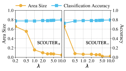
The relationship between , which controls the size of explanatory regions, and the classification accuracy is shown in Fig. 5 for ResNeSt 26 model with . A clear pattern is that the area sizes of both SCOUTER+ and SCOUTER- drop quickly with the increase of . However, there is no significant trend in the classification accuracy, which should be because the cross-entropy loss term works well regardless of .
Also, according to the visualization results in Figs. 2 and 3, a larger does not simply decrease the explanatory regions’ sizes. Instead, SCOUTER shifts its focus from some larger supports to fewer, smaller yet also decisive supports. For example, in the first row of Fig. 3, when is small, SCOUTER- can easily make a decision that the input image is not a cock because of unique feathers on the neck. With a larger , SCOUTER finds smaller combinations of supports (i.e., its wattle) and thus the explanation changes from the (larger) neck to the (smaller) wattle region.
We also summarize the classification performance of the FC classifier, SCOUTER+ (), and SCOUTER- () over ImageNet [6], Con-text [20], and CUB-200 [39] datasets in Table 3. The subsets with are adopted for ImageNet and CUB-200, while all 30 categories are used for the Con-text. The results show that SCOUTER can be generalized to different domains and has a comparable performance with the FC classifier over all datasets. Also, SCOUTER’s number of parameters is comparable to FC’s (more details in supplementary material).
One drawback of SCOUTER is that its training is unstable when . This is possibly because of the increasing difficulty in finding effective supports that consistently appear in all images of the same category but are not shared by other categories. This drawback limits the application of SCOUTER to small- or medium-sized datasets.
4.4 Case Study
SCOUTER uses the area loss, which constrains the size of support. This constraint can benefit some applications, including the classification of medical images, since small support regions can precisely show the symptoms and are more informative in some cases. Also, there was no method that could give the negative explanation but it is actually needed (doctors need reasons to deny some diseases). SCOUTER was designed upon these needs and is being tested in hospitals for glaucoma (Fig. 6), artery hardening (supplementary material), etc.
For glaucoma diagnosis, we tested SCOUTER with over a publicly available dataset, i.e., ACRIMA [9], which has two categories (normal and glaucoma). ResNeSt 26 is used as backbone. The results are shown in Table 4. We can see that both SCOUTER+ and SCOUTER- get better performances than the FC classifier. Besides, SCOUTER is preferred in this task as doctors are eager to know the precise regions in the optic disc that lead to the machine diagnosis. We can see that, in the visualization results in Fig. 6, SCOUTER shows more precise and reasonable explanations that locate on some vessels in the optic disc and show clinical meanings (vessel shape change due to the enlarged optic cup), which are verified by doctors. Although IBA also gives small regions, they cover some unrelated or uninformative locations. In addition, it is notable that the facts to admit category “Glaucoma” need not to match with the facts to deny “Normal”, as they are only subsets of the support sets and an on-purpose negative explanation is especially helpful for the doctors when the machine decisions are against their expectations.
| Models | ImageNet | Con-text | CUB-200 |
|---|---|---|---|
| ResNeSt 26 (FC) | 0.8080 | 0.6732 | 0.7538 |
| ResNeSt 26 (SCOUTER+) | 0.7991 | 0.6870 | 0.7362 |
| ResNeSt 26 (SCOUTER-) | 0.7946 | 0.6866 | 0.7490 |
| ResNeSt 50 (FC) | 0.8158 | 0.6918 | 0.7739 |
| ResNeSt 50 (SCOUTER+) | 0.8242 | 0.6943 | 0.7397 |
| ResNeSt 50 (SCOUTER-) | 0.8066 | 0.6922 | 0.7600 |
| ResNeSt 101 (FC) | 0.8255 | 0.7038 | 0.7804 |
| ResNeSt 101 (SCOUTER+) | 0.8251 | 0.7131 | 0.7428 |
| ResNeSt 101 (SCOUTER-) | 0.8267 | 0.7062 | 0.7643 |

5 Conclusion
An explainable classifier is proposed in this paper, with two variants, i.e., SCOUTER+ and SCOUTER-, which can respectively give positive or negative explanation of the classification process. SCOUTER adopts an explainable variant of the slot attention, namely, xSlot attention, which is also based on the self-attention. Moreover, a loss is designed to control the size of explanatory regions. Experimental results prove that SCOUTER can give accurate explanations while keeping good classification performance.
| Methods | AUC | Acc. | Prec. | Rec. | F1 | Kappa |
|---|---|---|---|---|---|---|
| FC | 0.9997 | 0.9857 | 0.9915 | 0.9831 | 0.9872 | 0.9710 |
| SCOUTER+ | 1.0000 | 1.0000 | 1.0000 | 1.0000 | 1.0000 | 1.0000 |
| SCOUTER- | 0.9999 | 0.9952 | 1.0000 | 0.9915 | 0.9957 | 0.9903 |
6 Acknowledgments
This work was supported by Council for Science, Technology and Innovation (CSTI), cross-ministerial Strategic Innovation Promotion Program (SIP), “Innovative AI Hospital System” (Funding Agency: National Institute of Biomedical Innovation, Health and Nutrition (NIBIOHN)). This work was also supported by JSPS KAKENHI Grant Number 19K10662, 20K23343, 21K17764, MHLW AC Program Grant Number 20AC1006, and JST CREST Grant Number JPMJCR20D3, Japan.
References
- [1] Nicolas Carion, Francisco Massa, Gabriel Synnaeve, Nicolas Usunier, Alexander Kirillov, and Sergey Zagoruyko. End-to-end object detection with transformers. arXiv preprint arXiv:2005.12872, 2020.
- [2] Jooyoung Chang, Jinho Lee, Ahnul Ha, Young Soo Han, Eunoo Bak, Seulggie Choi, Jae Moon Yun, Uk Kang, Il Hyung Shin, Joo Young Shin, et al. Explaining the rationale of deep learning glaucoma decisions with adversarial examples. Ophthalmology, 128(1):78–88, 2021.
- [3] Aditya Chattopadhay, Anirban Sarkar, Prantik Howlader, and Vineeth N Balasubramanian. Grad-CAM++: Generalized gradient-based visual explanations for deep convolutional networks. In IEEE WACV, pages 839–847, 2018.
- [4] Mark Chen, Alec Radford, Rewon Child, Jeff Wu, Heewoo Jun, Prafulla Dhariwal, David Luan, and Ilya Sutskever. Generative pretraining from pixels. In ICML, 2020.
- [5] Piotr Dabkowski and Yarin Gal. Real time image saliency for black box classifiers. In NeurIPS, pages 6967–6976, 2017.
- [6] Jia Deng, Wei Dong, Richard Socher, Li-Jia Li, Kai Li, and Li Fei-Fei. ImageNet: A large-scale hierarchical image database. In IEEE CVPR, pages 248–255, 2009.
- [7] Saurabh Desai and Harish G. Ramaswamy. Ablation-CAM: Visual explanations for deep convolutional network via gradient-free localization. In IEEE WACV, pages 972–980, 2020.
- [8] Jacob Devlin, Ming-Wei Chang, Kenton Lee, and Kristina Toutanova. BERT: Pre-training of deep bidirectional transformers for language understanding. arXiv preprint arXiv:1810.04805, 2018.
- [9] Andres Diaz-Pinto, Sandra Morales, Valery Naranjo, Thomas Köhler, Jose M Mossi, and Amparo Navea. CNNs for automatic glaucoma assessment using fundus images: an extensive validation. Biomedical Engineering Online, 18(1):29, 2019.
- [10] Ruth Fong, Mandela Patrick, and Andrea Vedaldi. Understanding deep networks via extremal perturbations and smooth masks. In IEEE ICCV, pages 2950–2958, 2019.
- [11] Ruth C Fong and Andrea Vedaldi. Interpretable explanations of black boxes by meaningful perturbation. In IEEE ICCV, pages 3429–3437, 2017.
- [12] Anirudh Goyal, Alex Lamb, Phanideep Gampa, Philippe Beaudoin, Sergey Levine, Charles Blundell, Yoshua Bengio, and Michael Mozer. Object files and schemata: Factorizing declarative and procedural knowledge in dynamical systems. arXiv preprint arXiv:2006.16225, 2020.
- [13] Yash Goyal, Ziyan Wu, Jan Ernst, Dhruv Batra, Devi Parikh, and Stefan Lee. Counterfactual visual explanations. In ICML, 2019.
- [14] Kaiming He, Xiangyu Zhang, Shaoqing Ren, and Jian Sun. Deep residual learning for image recognition. In IEEE CVPR, pages 770–778, 2016.
- [15] Mikael Henaff, Jason Weston, Arthur Szlam, Antoine Bordes, and Yann LeCun. Tracking the world state with recurrent entity networks. In ICLR, 2017.
- [16] Geoffrey Hinton, Oriol Vinyals, and Jeff Dean. Distilling the knowledge in a neural network. arXiv preprint arXiv:1503.02531, 2015.
- [17] Andrew G Howard, Menglong Zhu, Bo Chen, Dmitry Kalenichenko, Weijun Wang, Tobias Weyand, Marco Andreetto, and Hartwig Adam. MobileNets: Efficient convolutional neural networks for mobile vision applications. arXiv preprint arXiv:1704.04861, 2017.
- [18] Jie Hu, Li Shen, and Gang Sun. Squeeze-and-excitation networks. In IEEE CVPR, pages 7132–7141, 2018.
- [19] Gao Huang, Zhuang Liu, Laurens Van Der Maaten, and Kilian Q Weinberger. Densely connected convolutional networks. In IEEE CVPR, pages 4700–4708, 2017.
- [20] Sezer Karaoglu, Ran Tao, Jan van Gemert, and Theo Gevers. Con-Text: Text detection for fine-grained object classification. IEEE TIP, 26(8):3965–3980, 2017.
- [21] Jinkyu Kim and John Canny. Interpretable learning for self-driving cars by visualizing causal attention. In IEEE ICCV, pages 2942–2950, 2017.
- [22] Yann LeCun, Léon Bottou, Yoshua Bengio, and Patrick Haffner. Gradient-based learning applied to document recognition. Proceedings of the IEEE, 86(11):2278–2324, 1998.
- [23] Francesco Locatello, Dirk Weissenborn, Thomas Unterthiner, Aravindh Mahendran, Georg Heigold, Jakob Uszkoreit, Alexey Dosovitskiy, and Thomas Kipf. Object-centric learning with slot attention. arXiv preprint arXiv:2006.15055, 2020.
- [24] David Mascharka, Philip Tran, Ryan Soklaski, and Arjun Majumdar. Transparency by design: Closing the gap between performance and interpretability in visual reasoning. In IEEE CVPR, pages 4942–4950, 2018.
- [25] Daniel Omeiza, Skyler Speakman, Celia Cintas, and Komminist Weldermariam. Smooth Grad-CAM++: An enhanced inference level visualization technique for deep convolutional neural network models. arXiv preprint arXiv:1908.01224, 2019.
- [26] Niki Parmar, Ashish Vaswani, Jakob Uszkoreit, Lukasz Kaiser, Noam Shazeer, Alexander Ku, and Dustin Tran. Image transformer. In ICML, 2018.
- [27] Vitali Petsiuk, Abir Das, and Kate Saenko. RISE: Randomized input sampling for explanation of black-box models. In BMVC, 2018.
- [28] Zhongang Qi, Saeed Khorram, and Li Fuxin. Visualizing deep networks by optimizing with integrated gradients. In AAAI, volume 34, pages 11890–11898, 2020.
- [29] Marco Tulio Ribeiro, Sameer Singh, and Carlos Guestrin. Why should I trust you? Explaining the predictions of any classifier. In KDD, pages 1135–1144, 2016.
- [30] Karl Schulz, Leon Sixt, Federico Tombari, and Tim Landgraf. Restricting the flow: Information bottlenecks for attribution. In ICLR, 2020.
- [31] Ramprasaath R. Selvaraju, Michael Cogswell, Abhishek Das, Ramakrishna Vedantam, Devi Parikh, and Dhruv Batra. Grad-CAM: Visual explanations from deep networks via gradient-based localization. In IEEE ICCV, pages 618–626, 2017.
- [32] Avanti Shrikumar, Peyton Greenside, and Anshul Kundaje. Learning important features through propagating activation differences. In ICML, page 3145–3153, 2017.
- [33] Mingxing Tan and Quoc V Le. Efficientnet: Rethinking model scaling for convolutional neural networks. arXiv preprint arXiv:1905.11946, 2019.
- [34] Ashish Vaswani, Noam Shazeer, Niki Parmar, Jakob Uszkoreit, Llion Jones, Aidan N Gomez, Łukasz Kaiser, and Illia Polosukhin. Attention is all you need. In NeurIPS, pages 5998–6008, 2017.
- [35] Haofan Wang, Rakshit Naidu, Joy Michael, and Soumya Snigdha Kundu. SS-CAM: Smoothed Score-CAM for sharper visual feature localization. arXiv preprint arXiv:2006.14255, 2020.
- [36] Haofan Wang, Zifan Wang, Mengnan Du, Fan Yang, Zijian Zhang, Sirui Ding, Piotr Mardziel, and Xia Hu. Score-CAM: Score-weighted visual explanations for convolutional neural networks. In IEEE CVPR Workshops, pages 24–25, 2020.
- [37] Huiyu Wang, Yukun Zhu, Bradley Green, Hartwig Adam, Alan Yuille, and Liang-Chieh Chen. Axial-deeplab: Stand-alone axial-attention for panoptic segmentation. arXiv preprint arXiv:2003.07853, 2020.
- [38] Pei Wang and Nuno Vasconcelos. SCOUT: Self-aware discriminant counterfactual explanations. In IEEE CVPR, pages 8981–8990, 2020.
- [39] Peter Welinder, Steve Branson, Takeshi Mita, Catherine Wah, Florian Schroff, Serge Belongie, and Pietro Perona. Caltech-UCSD Birds 200. Technical Report CNS-TR-2010-001, California Institute of Technology, 2010.
- [40] Zbigniew Wojna, Alex Gorban, Dar-Shyang Lee, Kevin Murphy, Qian Yu, Yeqing Li, and Julian Ibarz. Attention-based extraction of structured information from street view imagery. In ICDAR, pages 844–850, 2017.
- [41] Zhibiao Wu and Martha Palmer. Verbs semantics and lexical selection. In ACL, page 133–138, 1994.
- [42] Ning Xie, Farley Lai, Derek Doran, and Asim Kadav. Visual entailment: A novel task for fine-grained image understanding. arXiv preprint arXiv:1901.06706, 2019.
- [43] Ning Xie, Gabrielle Ras, Marcel van Gerven, and Derek Doran. Explainable deep learning: A field guide for the uninitiated. arXiv preprint arXiv:2004.14545, 2020.
- [44] Chih-Kuan Yeh, Cheng-Yu Hsieh, Arun Suggala, David I Inouye, and Pradeep K Ravikumar. On the (in)fidelity and sensitivity of explanations. In NeurIPS, pages 10967–10978, 2019.
- [45] Matthew D Zeiler and Rob Fergus. Visualizing and understanding convolutional networks. In ECCV, pages 818–833, 2014.
- [46] Hang Zhang, Chongruo Wu, Zhongyue Zhang, Yi Zhu, Zhi Zhang, Haibin Lin, Yue Sun, Tong He, Jonas Muller, R. Manmatha, Mu Li, and Alexander Smola. ResNeSt: Split-attention networks. arXiv preprint arXiv:2004.08955, 2020.
- [47] Jianming Zhang, Sarah Adel Bargal, Zhe Lin, Jonathan Brandt, Xiaohui Shen, and Stan Sclaroff. Top-down neural attention by excitation backprop. International Journal of Computer Vision, 126(10):1084–1102, 2018.
- [48] Quanshi Zhang, Yu Yang, Haotian Ma, and Ying Nian Wu. Interpreting CNNs via decision trees. In IEEE CVPR, pages 6261–6270, 2019.
- [49] Bolei Zhou, Aditya Khosla, Agata Lapedriza, Aude Oliva, and Antonio Torralba. Learning deep features for discriminative localization. In IEEE CVPR, pages 2921–2929, 2016.
SCOUTER: Slot Attention-based Classifier for Explainable Image Recognition
(Supplementary Material)
1 Computational Costs
Table 1 gives the cost comparison of SCOUTER and FC classifier. We can see that, compared with the FC classifier, SCOUTER requires a similar computational cost (slightly higher) and a similar number of parameters (slightly lower). The increase in the computational cost (flops) is because the xSlot module has some small FC layers (i.e., and ), GRU, and some matrix calculations. However, as shown in the lower part of Fig. 1, this is not very significant.
On the other hand, as shown in the upper part of Fig. 1, SCOUTER has more parameters than the FC classifier when is roughly in . This is because the FC layers and GRU, which are shared among all slots, have a certain number of parameters. For , SCOUTER uses fewer parameters than the FC classifier because there are only ( in our implementation) learnable parameters for each category. This is much less than the parameter size of the FC classifier, which usually needs much more parameters per class ( parameters for ResNet 50).
Comparing to the differences in the computation costs and the numbers of parameters of different backbone models, the additional cost of SCOUTER is almost negligible.
2 Components of xSlot Attention Module
In SCOUTER, we adopt a variant of the slot attention [23]. We make some essential modifications to several components in order to enable explainable classification, while other components, i.e. the gated recurrent unit (GRU) and position embedding (PE), remain unchanged, whose effects on the classification as well as the explainability are unexplored. To test the performance of the SCOUTER with and without these components, we consider two variants of SCOUTER. The first one is the SCOUTER without GRU, in which we replace the GRU component, which is used to update slot weights, with an average operation. The second variant is the SCOUTER without PE, where flattened input features are directly used without adding position information.
In Table 2, we show the performances of SCOUTER+ and SCOUTER- as well as their variants in several performance metrics including computation costs, classification accuracy, and explainability. We can see that SCOUTER with all the components gets better results in most metrics than the variants, except for computation costs. The absence of GRU or PE not only causes a decrease of the classification accuracy, but also some deterioration on all explainability metrics, which proves their necessity.
| Models | Params (M) | Flops (G) | |||
|---|---|---|---|---|---|
| FC | SCOUTER | FC | SCOUTER | ||
| ResNet 26 [14] | 14.1511 | 14.1298 | 3.4238 | 3.4565 | |
| ResNet 50 [14] | 23.7129 | 23.6916 | 5.9830 | 6.0171 | |
| ResNeSt 26 [46] | 15.2253 | 15.2041 | 5.1803 | 5.2130 | |
| ResNeSt 50 [46] | 25.6391 | 25.6179 | 7.7430 | 7.7762 | |
| DenseNet 121 [19] | 7.0564 | 7.0719 | 3.7536 | 3.7805 | |
| DenseNet 169 [19] | 12.6510 | 12.6435 | 4.4396 | 4.4683 | |
| MobileNet 75 [17] | 1.1194 | 0.6537 | 0.0563 | 0.0812 | |
| MobileNet 100 [17] | 4.3301 | 3.0859 | 0.3154 | 0.3421 | |
| SeResNet 18 [18] | 11.3169 | 11.3509 | 2.6473 | 2.6726 | |
| SeResNet 50 [18] | 26.2439 | 26.2226 | 5.6758 | 5.7098 | |
| EfficientNet B2 [33] | 7.8419 | 7.8437 | 1.0250 | 1.0564 | |
| EfficientNet B5 [33] | 28.5457 | 28.5244 | 3.6391 | 3.6721 | |

| Explanation Type | Variants | Computational Costs | Classification | Explainability | |||
|---|---|---|---|---|---|---|---|
| Params (M) | Flops (G) | Accuracy | Precision | IAUC | DAUC | ||
| Positive | SCOUTER+ | 15.2041 | 5.2130 | 0.7991 | 0.9257 | 0.7647 | 0.2713 |
| w.o. GRU | 15.1791 | 5.1901 | 0.7961 | 0.9219 | 0.7456 | 0.2866 | |
| w.o. PE | 15.2041 | 5.2130 | 0.7974 | 0.8973 | 0.7557 | 0.3002 | |
| Negative | SCOUTER- | 15.2041 | 5.2130 | 0.7946 | 0.8101 | 0.6730 | 0.7333 |
| w.o. GRU | 15.1791 | 5.1901 | 0.7910 | 0.7904 | 0.5959 | 0.7529 | |
| w.o. PE | 15.2041 | 5.2130 | 0.7903 | 0.8067 | 0.6141 | 0.7661 | |
3 Classification Performance when
Training of SCOUTER becomes unstable when the category number of the ImageNet [6] subsets is larger than . One possible reason is that it is difficult to find consistent and discriminative supports when there are many categories. Fig. 2 shows the classification performance when . The number of independent runs of training is increased to as the training process becomes unstable and often results in failures (low classification accuracy) when . is set to . ResNeSt 26 [46] is adopted as the backbone, with batch size of and training epoch number of (both are same as the settings of the experiments in the main paper). We can see that, although sometimes SCOUTER+ and SCOUTER- can achieve similar performance with the FC classifier when , they become significantly unstable with the increase of category number . As stated in the main paper, SCOUTER can only be used in small-or medium-sized datasets due to this issue.

4 Inter-and Intra-Category Explanation
To better understand (i) what supports SCOUTER uses as the basis for its decision making, (ii) how these supports can be differentiated among different categories, and (iii) whether they are being consistent for images in the same category, we give some additional visualization on the MNIST dataset [22] in Figs. 3 and 4 for SCOUTER+ and SCOUTER-, respectively. MNIST is adopted here as similarities and dissimilarities among categories (digits) are obvious and are easier to understand than ImageNet. In these two figures, (a) is for the inter-category visualization, which shows what the supports for the “Predicted” category look like given the image of the “Actual” category. Whereas, (b) is for intra-category visualization, which shows the support for different images of the same category. For the latter, we use the digit 6 as an example and the first ten samples of category 6 in the test set of MNIST are used.
In the inter-category visualization in Fig. 3, we can see that SCOUTER+ successfully finds supports for the images of ground-truth (GT) categories. Notably, it also finds weaker supports for some categories with similar appearances, e.g., the supports for the prediction of “why 5 is 6” (as the lower half of this hand-wrote 5 digit is a little confusing and is very close to the lower part of 6), as well as the prediction of “why 0 is 9” and “why 8 is 9” (both 0 and 8 have a circle like the one in 9).
Similarly, in Fig. 4, we can see that SCOUTER- finds no supports for the images of the GT categories, while it finds strong supports for the non-GT categories. As digit recognition is an easy task, SCOUTER- can use some very simple supports to deny most non-GT categories. For example, in the prediction of “why 1 is not [non-GT categories]”, all the slots of SCOUTER- find that the top end of the vertical stroke is 1’s unique pattern, thus, they can deny all other categories with this support. Among some visually similar categories, the negative explanations are more informative. For example, in the visualization of “why 9 is not 1” and “why 9 is not 7”, SCOUTER- precisely highlights the discriminative regions, without which 9 will look like the other two digits.
Also, in intra-category visualization, both SCOUTER+ and SCOUTER- show consistent supports for the images of the same category. When predicting “why 6 is 6”, SCOUTER+ always looks at the region close to the crossing point of the bottom circle and vertical stroke. For explanation “why 6 is not 2”, SCOUTER- always recognizes the presence of vertical stroke, which does not exist in the digit 2, as well as the missing of the bottom horizon stroke, which is essential for 2.
5 Some More Visualizations
In this section, we show more visualization results for ImageNet using SCOUTER and competing methods, including I-GOS [28], IBA [30], CAM [49], GradCAM [31], GradCAM++ [3], S-GradCAM++ [25], Score-CAM [36], SS-CAM [35], and Extremal Perturbation [10].
Subsets with categories are used for training and visualization. Besides the first categories (as used in the main paper), we also use several other subsets (with the same category number) in the ImageNet dataset, in order to provide visualizations with more diversity. Figs. 5 and 6 give examples of the positive explanation, while Fig. 7 gives examples of the negative explanation.
Among the positive explanations, we can see that SCOUTER+ can find reasonable and precise supports. Especially for the image of “parallel bars”, SCOUTER+ can provide an explanatory region along the horizon bar. In addition, SCOUTER- with the least similar class (LSC) also finds supports on the foreground objects, which can be used to deny the LSC categories but are not enough for admitting the GT category, which conforms the quantitative results in the main paper.
Moreover, as shown in Fig. 7, SCOUTER- can give very detailed explanations when different categories with high visual similarities, e.g., the differences in the eyes and ears between “Labrador retriever” and “golden retriever”, and the differences of the horn between “water ox” and “ox”.
Figs. 8 and 9 show some more examples of two medical applications (glaucoma diagnosis and artery hardening diagnosis). We can see that SCOUTER+ and SCOUTER- perform well in both tasks.


