Scene-aware Human Pose Generation using Transformer
Abstract.
Affordance learning considers the interaction opportunities for an actor in the scene and thus has wide application in scene understanding and intelligent robotics. In this paper, we focus on contextual affordance learning, i.e., using affordance as context to generate a reasonable human pose in a scene. Existing scene-aware human pose generation methods could be divided into two categories depending on whether using pose templates. Our proposed method belongs to the template-based category, which benefits from the representative pose templates. Moreover, inspired by recent transformer-based methods, we associate each query embedding with a pose template, and use the interaction between query embeddings and scene feature map to effectively predict the scale and offsets for each pose template. In addition, we employ knowledge distillation to facilitate the offset learning given the predicted scale. Comprehensive experiments on Sitcom dataset demonstrate the effectiveness of our method.
1. Introduction
Affordance learning (Gibson, 1979) is a long-standing and significant topic, which studies the possible interactions that an actor is allowed to have with the environment. In application, affordance learning covers numerous types of tasks, e.g., contextual affordance learning (Lopes et al., 2007; Ugur et al., 2011), functionality understanding (Zhu et al., 2015; Shiraki et al., 2014), affordance classification/detection/segmentation (Varadarajan and Vincze, 2013; Grabner et al., 2011; Eigen and Fergus, 2015). In this paper, we focus on contextual affordance learning, which uses affordance as context for the specified tasks, e.g., scene-aware human pose generation. Learning such affordance not only allows actors to better interact in the scene, but also offers considerate feedback to the scene designers. Therefore, contextual affordance learning has profound benefit for content analysis (Gupta et al., 2011), intelligent robotics (Lopes and Santos-Victor, 2005), and scene understanding (Castellini et al., 2011).

In this work, we focus on learning the affordance between human and scene (Wang et al., 2017), i.e., how we can put a human in a scene. As shown in Figure 1 (a), given a 2D scene image and a target point, we need to generate a human pose that reasonably interacts with the scene at the target point. Scene-aware human pose generation is actually a challenging task, because the model needs to understand the human, the scene, and the interaction between them. For example, in the case of Figure 1 (a), the model should comprehend the function of sofa, know the possible poses of human body, place the human body on the sofa, and adjust the human keypoints according to the geometry of sofa reasonably. As shown in Figure 1 (b), a hypothetical human could sit in the sofa with the back against the backrest and hams on the cushion. Despite the significance of this task, there are only few efforts in this field. Previous methods and intuitive solutions of this task could be divided into two categories depending on whether using pose templates. Non-template-based methods are similar to pose estimation methods, which directly predict the location of each keypoint. Template-base methods generate pose based on pre-defined templates. Wang et. al. (Wang et al., 2017) constructed a dataset by collecting ground-truth poses at target points from video frames of sitcoms and proposed to use VAE (Kingma and Welling, 2014) to predict the scale and offsets of target compared with the chosen pose template.
Inspired by the great success of transformer in a wide range of computer vision tasks (Dosovitskiy et al., 2021; Carion et al., 2020; Cheng et al., 2021), we propose an end-to-end trainable network based on transformer. Previous works (Carion et al., 2020; Cheng et al., 2021) use query embedding to represent the potential object or category, while we use query embedding to represent the pose template. As shown in Figure 1 (c), we set a number of pose templates in our model, which are prepared by using clustering algorithm to find representative poses in the training set. Each pose template is associated with one template embedding to interact with the scene. Specifically, the -th template embedding represents the -th pose template. Given a 2D scene image, we first extract its feature map via a backbone network and upsampling module, based on which the compatibility score of each pose template is predicted. Because there might be multiple pose templates which are reasonable for the input scene image, we introduce self-training strategy for compatibility score learning. Then, each pose template interacts with the scene by feeding its query embedding and the scene feature map into two cascaded transformer modules (Vaswani et al., 2017) to obtain the pose scale and offsets. Specifically, the query embedding first interacts with the whole feature map to predict the scale according to the global context, and then interacts with the local feature map to predict the offsets according to the fine-grained context. In this way, all plausible pose templates directly and parallelly interact with the scene image for predicting their scales and offsets.
For the model training, we use binary entropy loss to supervise compatibility score, and use MSE loss to supervise scale and offsets. In order to facilitate the offset learning given the predicted scale, we introduce knowledge distillation in our model. Moreover, we also supervise the refinement of templates that are not ground-truth but might fit the scene by adversarial loss.
We conduct comprehensive experiments on Sitcom affordance dataset (Wang et al., 2017) with in-depth analyses to demonstrate the effectiveness of our method. Our contributions can be summarized as: 1) we propose an end-to-end trainable transformer network for scene-aware human pose generation; 2) we propose to facilitate the offset learning with knowledge distillation; 3) extensive experiments on Sitcom affordance dataset show the advantage of our method against state-of-the-art baselines.
2. Related Works
2.1. Affordance Learning
The concept of affordance (Gibson, 1979) is first proposed by ecological psychologist James Gibson, which describes “opportunities for interactions” of environment. Recently, affordance learning has included extensive applications, including contextual affordance learning (Lopes et al., 2007; Ugur et al., 2011), functionality understanding (Zhu et al., 2015; Shiraki et al., 2014), affordance classification (Varadarajan and Vincze, 2013; Ugur et al., 2014), affordance detection (Grabner et al., 2011; Moldovan and De Raedt, 2014), affordance segmentation (Eigen and Fergus, 2015; Roy and Todorovic, 2016), etc. Our work is more related to contextual affordance learning, which employs affordance relationships as context for associated tasks. For examples, Lopes et al. (Lopes and Santos-Victor, 2005) proposed to use contextual affordance as prior information to enhance gesture recognition and decrease ambiguities according to motor terms. Castellini et al. (Castellini et al., 2011) employed affordance as visual features and motor features to benefit the object recognition task. Gupta et al. (Gupta et al., 2011) learned affordance in indoor images to detect the workspace according to human poses. Recently, Wang et al.(Wang et al., 2017) adopted the scene affordance as context for human pose generation. In this paper, we also focus on generating a scene-aware human pose as in (Wang et al., 2017).
2.2. Object Placement
Human could be considered as a specific object, and thus our task is also related to the field of object placement, which is an important subtask of image composition (Niu et al., 2021). Early methods (Tan et al., 2018; Tripathi et al., 2019; Li et al., 2019; Zhang et al., 2020a, b) mainly depended on explicit rules for placing foreground objects in background images, while recent methods (Liu et al., 2021; Zhang et al., 2020a; Tripathi et al., 2019; Zhou et al., 2022) employed deep learning for object placement. To name a few, Lin et al. (Lin et al., 2018b) proposed to use spatial transformer networks to learn geometric corrections to warp composite images to appropriate layouts. PlaceNet (Zhang et al., 2020a) predicted a diverse distribution for common sense locations to place the given foreground object on the background scene. TERSE (Tripathi et al., 2019) proposed to train synthesizer and target networks in adversarial manner for plausible object placement. Lee et al. (Lee et al., 2018) employed a two-stage pipeline to determine where to place objects and what classes to place. Azadi et al. (Azadi et al., 2020) proposed a self-consistent composition-by-decomposition network to learn to place objects, based on the insight that a successful composite image could be decomposed back into individual objects. Most recently, Zhou et al. (Zhou et al., 2022) treated object placement as a graph completion problem and proposed a graph completion module to solve the task. The work (Niu et al., 2022) proposed to identify the reasonable placements using a discriminative approach, by predicting the rationality scores of all scales and locations. In our task, the model needs to understand the scene and the human-scene interaction, and generate reasonable human poses from a large searching space, which is a very challenging task.
2.3. Human Pose Estimation and Generation
Human pose estimation and generation has extensive applications and thus has attracted wide attention in decades. As for human pose estimation, conventional methods (Dantone et al., 2013; Sapp et al., 2010; Sun et al., 2012; Wang and Li, 2013; Wang and Mori, 2008) employed probabilistic graphical models or the pictorial structure models to represent the relations between human body parts. Recent human pose estimation methods (Artacho and Savakis, 2020; Cheng et al., 2020; Lin et al., 2018a; Su et al., 2019; Tang et al., 2019; Li et al., 2021) have achieved significant progress by using deep learning models. Technically, there are roughly two groups of pipelines for pose estimation: regression-based (Toshev and Szegedy, 2014; Carreira et al., 2016; Sun et al., 2017; Luvizon et al., 2019) and heatmap-based (Wei et al., 2016; Chu et al., 2017; Newell et al., 2016; Martinez et al., 2017). As for human pose generation, recent works generate human pose conditioned on past poses in video (Walker et al., 2017), textual description (Hong et al., 2022), or video motion (Rempe et al., 2021). Except for (Wang et al., 2017), there are few works generating human poses skeletons conditioned on 2D scene images.
3. Method
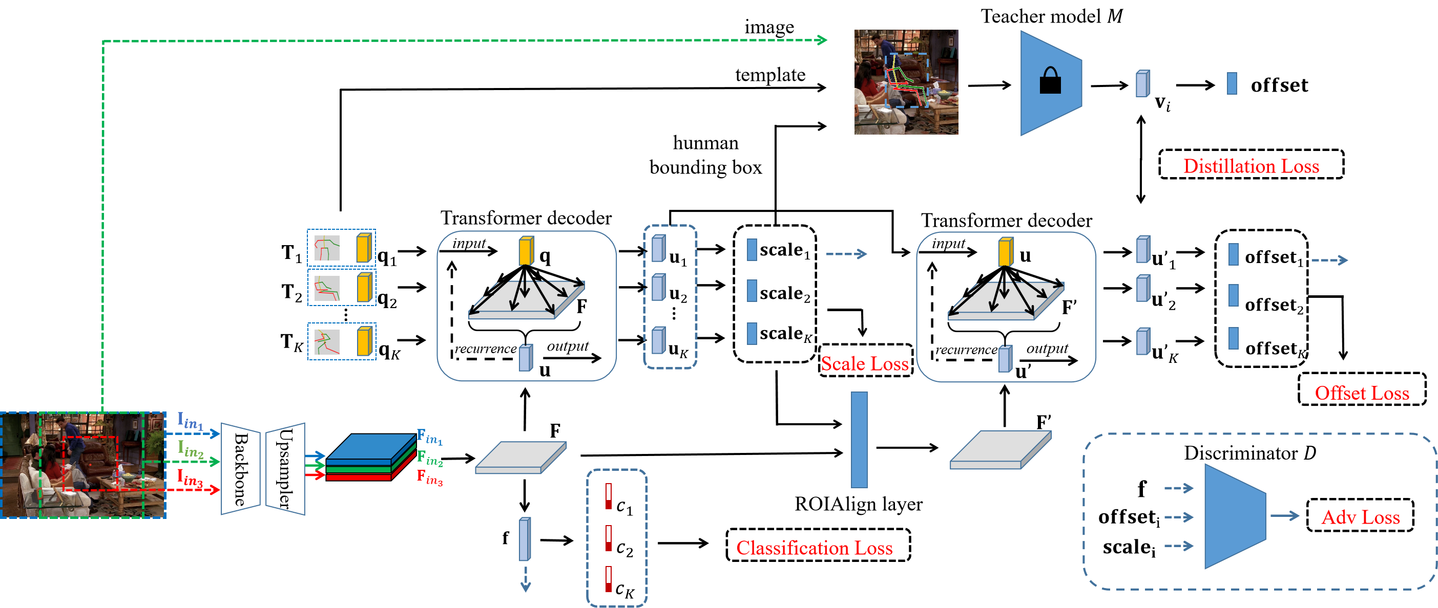
Given a full scene image and a target point , we need to generate a reasonable human pose with its enclosing rectangle centered at o. As in (Wang et al., 2017; Andriluka et al., 2014), the human pose P is represented by keypoints (e.g., right ankle, pelvis), that is, with being the -th keypoint. The whole pipeline of our method is shown in Figure 2, which uses pose templates and employs two cascaded transformer modules to model the interaction between each pose template and the input scene to produce the affordance pose. Each component of our method will be introduced in the following.
3.1. Pose Template Construction
Considering that the definition of affordance learning in our task is how a hypothetical human could interact with the scene, we construct a number of representative pose templates in training set to facilitate the interaction modeling between the hypothetical human and scene image. Specifically, we first normalize all ground-truth (GT) training poses. Then, we apply K-means clustering and further select representative cluster centers as pose templates by considering poses as -dim vectors and using Euclidean distance as distance metric ( by default).
For pose normalization, we define the box centered at with side length as the unit box, denoted as . We also define a function to output the enclosing box of its input pose, i.e., by fetching the maximum and minimum x,y-coordinates of keypoints in the input pose. For each GT training pose , we compute its normalized pose by
| (1) |
where is a linear deformation function defined by mapping box to box and could be used to deform the keypoints of input pose. In this way, each normalized pose will have the unit box as its enclosing box, i.e., . In our method, these pose templates will be refined to affordance pose according to the interaction with scene image.
3.2. Scene Image Preparation
When the scene image and target point o are given, we prepare three forms of input images to leverage multi-scale information following (Wang et al., 2017). As shown in Figure 2, the first input image is the whole image offering global context of scene image. The second input image is a square patch centered at o and the side length is the height of the scene image, which captures the scene context around the target location. The final input image is also a square patch but in half height to provide high-resolution information of scene context. We re-scale three images to the same size , which is set as in implementation. For each sample, the ground-truth label consists of three parts: class , scale , and normalized pose . Class is the index of nearest pose template. We calculate the scale as the actual height and width divided by the actual height of .
3.3. Network Architecture
As shown in Figure 2, our network consists of four modules: 1) a foundation network module, which generates feature map of the input scene image and predicts the compatibility score of each pose template; 2) a scale transformer module, which contains several transformer decoder layers as in (Carion et al., 2020; Cheng et al., 2021) and an MLP prediction head; 3) an offset transformer module, which is similar to scale transformer module in architecture; 4) a knowledge distillation module, which is a pre-trained offset regression network.
Foundation network module. Foundation network module consists of a backbone network, an upsampling network, and a classifier. We employ ResNet- (He et al., 2016) as our backbone network. Because the spatial resolution of ResNet- output () is not enough for fine-grained context, we append it with an upsampling module to yield relatively high-resolution feature map. Specifically, similar to the pixel decoder in MaskFormer (Cheng et al., 2021), we gradually upsample the feature map and sum it with the intermediate feature map of the corresponding resolution from the backbone network. As aforementioned, for each full scene image, we have three forms of input image , , and , leading to three feature maps , , and after the foundation network module. Finally, three feature maps are concatenated and squeezed via convolutional layer to produce the scene feature map , in which in our implementation. In this way, the scene feature map contains coarse context, fine context, and global context, which provide complementary information for later scene-aware human pose generation. The feature map will pass a global pooling layer and then pass a full-connected layer to get the binary compatibility score for each of pose templates.
Scale transformer module. Given the feature map of scene image F and each pose template , we use transformer module to model the interaction between pose templates and scene, which can be formulated as
| (2) |
where is a transformer module as in (Carion et al., 2020; Cheng et al., 2021) and is the interacted embedding decoded from the -th template embedding . Specifically, the transformer module consists of transformer decoder layers. In the transformer module, the embedding of each pose template interacts with each pixel of scene feature map, which facilitates human pose scale prediction through the global context of the whole image. We then use an MLP to predict the scale (two scale values along the x-axis and y-axis respectively) of each pose template based on the interacted embedding .
Offset transformer module. After getting the predicted scale, we compute the enclosing human bounding box and pay more attention to the features within the human bounding box. Specifically, we crop the feature map of the enclosing box region and resize it to the size of original feature map () using a ROIAlign layer. The resized feature map is then used as the key and value of the transformer module, which can be formulated as
| (3) |
where is the resized feature map within human bounding box. The transformer module consists of transformer decoder layer. Then we use a MLP to predict the coordinate offsets .
Next we will show how to get the actual output pose prediction given a scene image. As shown in Figure 3, the relative coordinate (resp., ) on -axis corresponds to the left (resp., right) boundary of input image . Similarly, the relative coordinate (resp., ) on -axis corresponds to the bottom (resp., top) boundary of input image . We first add the offsets to the pose template (i.e., ) to obtain the raw affordance pose. Then, we normalize this pose by (see Eq 1) to ensure that the center of predicted affordance pose is at the target point o. Finally, we scale the pose with , where denotes the scales of all keypoints and all keypoints share the same ,-scale value . As for the range of offset prediction, we assert that any offset for normalized pose should not exceed a certain range, which is set to the size of normalized box, so we define the offset for normalized pose. We also observe that the max height of ground-truth pose does not exceed twice the image height, so we set the scale to ensure that the final predicted pose is in range of . Specifically, we refine each pose template to get the final pose by
| (4) |
Distillation module We introduce a distillation module to improve the performance of offset prediction. Because our model can be seen as a multi-task model, introducing a teacher model that focuses on predicting offsets given the scale and pose template can effectively help our model search for optimal solutions in a smaller range and converge faster. Specifically, we employ ResNet- (He et al., 2016) as our teacher network. During the pre-training phase, we first use ground-truth scale to derive the human bounding box, then we can fit the ground-truth pose template into the bounding box and get the heatmap of each keypoint. Finally, we concatenate the heatmaps and the scene image as the model input. The teacher model predicts an offset vector, based on which we can get the corresponding predicted pose and use loss to supervise the model during pre-training.
During the training phase of our model, the keypoint heatmaps are generated by the ground-truth pose template and predicted scale from scale transformer module . Provided with keypoint heatmaps, we use fixed pre-trained teacher model to extract the feature vector . Recall that in our main network, offset transformer embedding accounts for offset prediction. Therefore, we realize knowledge distillation by narrowing the distance between offset transformer embedding and .
3.4. Training with Pose Mining
In existing dataset Sitcom, each training sample is only annotated with one ground-truth pose, corresponding to one pose template. However, other pose templates might also be plausible for this scene image. Therefore, we employ self-training to mine more reasonable human poses in a scene. Specifically, we design a multi-stage training strategy. In the first stage, we assign each sample its nearest pose template as its ground-truth class and train our model. After that, we change the label to positive if the trained model of the previous stage predicts a compatibility score higher than a threshold (i.e., ). The training moves on to the next stage when the test classification accuracy begins to decrease, and stops when the labels no longer change. We apply binary cross-entropy loss to supervise the predicted compatibility scores:
| (5) |
where is the compatibility score for the -th pose template, is the label of the -th pose template ( if the -th pose template is positive), is the weight to balance the quantity differences between positive and negative categories of the -th pose template in dataset, and is the binary cross-entropy loss.

Though multiple pose templates could be classified as positive, the ground-truth poses and pose templates are unique for each sample. Therefore, we only apply the refinement loss to the ground-truth pose template. The loss functions for the two refinement (scale and offsets) predictions could be formulated as
| (6) | ||||
| (7) |
We apply the distillation loss to the output embedding of ground-truth pose template in offset transformer module, which can be formulated as
| (8) |
where is the output embedding of offset transformer decoder, is the output embedding of teacher model.
Besides the single ground-truth pose template, there could be other positive pose templates. We apply an adversarial loss to these templates to ensure the quality of output poses. We use to denote the concatenation of three vectors, in which f is the feature vector after average pooling layer in foundation network module. is fed into the discriminator as input. The adversarial loss can be formulated as
| (9) |
where the discriminator is an MLP and predicts whether the input is from ground-truth template, is the index which satisfies and .
Therefore, the total training objective of our model is
| (10) |
where includes the model parameters of discriminator and includes the other model parameters. , , , and are hyper-parameters for balancing loss items. In our experiments, we set , , , and via cross-validation.
In the inference stage, we sort the predicted poses according to their compatibility scores , and select the poses with top compatibility scores as our final prediction.
4. Experiments
4.1. Dataset
We conduct experiments on Sitcom affordance dataset (Wang et al., 2017). The training samples are collected from the TV series of “How I Met Your Mother”, “The Big Bang Theory”, “Two and A Half Man”, “Everyone Loves Raymond”, “Frasier” and “Seinfeld”, consisting of k accurate poses over k different scenes. The test samples are collected from “Friends”, consisting of k accurate poses over k different scenes. Each scene image is annotated with one or more target location points and each target point has one annotated ground-truth pose with keypoints.

4.2. Evaluation
We use three evaluation metrics in our experiments, i.e., PCK (Percentage of Correct Keypoints), MSE (mean-square error), and user study.
PCK is a common metric used in pose estimation (Artacho and Savakis, 2020; Li et al., 2021; Cheng et al., 2020), which indicates the percentage of correctly predicted keypoints that fall within a certain distance threshold of the ground-truth. In our task, we choose [email protected] as in (Artacho and Savakis, 2020), which refers to a threshold of of the torso diameter (the distance between left hip and right shoulder, corresponding to the -rd point and the -th point in Sitcom dataset).
MSE measures the mean-square error between the predicted pose and GT pose. Specifically, we compute the mean-square error using the normalized coordinates which are divided by the heights of corresponding images, considering that the sizes of testing images may be quite different.
User study is conducted with voluntary participants by comparing the poses generated by different methods. For each test sample, every participant chooses the method producing the most reasonable pose. The score of each method is defined as the frequency that this method is chosen as the best one.
4.3. Implementation Details
For the network architecture, we use ResNet- (He et al., 2016) pretrained on ImageNet (Deng et al., 2009) as our backbone network and follow the setting of transformer module in (Cheng et al., 2021) for the two transformer modules. For the MLP settings in the prediction head of two transformer modules, the first hidden layers in pose offset and scale prediction head have hidden dimension of with ReLU activate function. The last layer of offset prediction is followed by a tanh function, while the last layer of scale prediction is followed by a sigmoid function. During the training stage, we apply SGD optimizer with learning rate and weight decay . A learning rate multiplier of is applied to backbone network and is applied to other modules of model. The batch size is set to . For the system environment, we use Python and Pytorch (Paszke et al., 2017). We conduct experiments on Ubuntu with Intel(R) Xeon(R) CPU v @ GHz CPU and four NVIDIA GeForce GTX Ti GPUs. The random seed is set as for all experiments unless stated otherwise.
| Model | PCK | MSE | User Study | ||||
|---|---|---|---|---|---|---|---|
| Top-1 | Top-3 | Top-5 | Top-1 | Top-3 | Top-5 | ||
| Heatmap | 0.363 | - | - | 53.45 | - | - | 0.025 |
| Regression | 0.386 | - | - | 51.29 | - | - | 0.037 |
| Wang et al. (Wang et al., 2017) | 0.401 | 0.432 | 0.458 | 46.65 | 44.49 | 43.17 | 0.225 |
| Unipose (Artacho and Savakis, 2020) | 0.387 | - | - | 46.78 | - | - | 0.071 |
| PRTR (Li et al., 2021) | 0.408 | - | - | 45.72 | - | - | 0.127 |
| PlaceNet (Zhang et al., 2020a) | 0.060 | 0.082 | 0.107 | 377.78 | 375.92 | 371.60 | 0 |
| GracoNet (Zhou et al., 2022) | 0.380 | 0.472 | 0.473 | 49.60 | 43.48 | 43.35 | 0.110 |
| Ours | 0.414 | 0.498 | 0.533 | 44.86 | 41.91 | 39.42 | 0.405 |

4.4. Qualitative Analyses
To provide in-depth analyses on how our model performs, we visualize the top- confident pose templates and the corresponding generated poses in Figure 4. From the visualizations, we could see that our model could not only choose pose templates suitable for the input scene image but also refine them to reasonable affordance poses. Taking the first row as example, our model produces high compatibility scores for all sitting pose templates, and then our model refines it to an affordance pose naturally sitting on the sofa. More qualitative analyses are left to Supplementary.
4.5. Comparison with Prior Works
Baseline Setting. We compare with the following representative baselines: two simple baselines, Wang et al. (Wang et al., 2017), pose estimation methods, and object placement methods.
1) Heatmap is a basic method producing keypoint heatmap. Specifically, we concatenate three feature maps , , and after the ResNet- (He et al., 2016) backbone network and upsampling module with upsampled resolution of . Then, the concatenated feature maps are fed into a convolution layer to produce an -channel keypoint heatmap.
2) Regression is also a intuitive method directly predicting the coordinates of human pose joints. We perform spatial average pooling on the concatenated feature maps which are the same as that in Heatmap baseline and send the pooled feature to a fully-connected layer to produce a -dim vector.
3) Wang et al. (Wang et al., 2017) is a two-stage approach for scene-aware human pose generation based on pose templates. In the first stage, it classifies the scene into one of pose templates which are the same as ours by sending the concatenated feature maps to a spatial average pooling layer and a linear classifier. In the second stage, it employs VAE (Kingma and Welling, 2014) to produce the deformations based on latent code, one-hot pose label vector, and the concatenated feature maps.
4) Unipose (Artacho and Savakis, 2020) and PRTR (Li et al., 2021) belong to pose estimation methods. Unipose (Artacho and Savakis, 2020) is a unified framework based on ”Waterfall” Atrous Spatial Pooling architecture. PRTR (Li et al., 2021) is the first transformer-based model used in pose estimation tasks, which regards query embedding as keypoint hypothesis and generates the final pose by finding a match.
5) PlaceNet (Zhang et al., 2020a) and GracoNet (Zhou et al., 2022) are two state-of-the-art methods in object placement task. To adapt the model to our task, we remove the encoder of foreground in these models and replace foreground feature vector with a learnable embedding.
In these methods, we use the same backbone as ours to extract the image feature map.
Quantitative Comparison. We first conduct quantitative comparison to precisely measure the discrepancies to GT poses in test set. Specifically, in our method and Wang et al. (Wang et al., 2017), we obtain top- confident predicted poses with highest compatibility scores and calculate their PCK/MSE, after which the predicted pose achieving the optimal PCK/MSE is used for evaluation. in PlaceNet(Zhang et al., 2020a) and GracoNet (Zhou et al., 2022), there are only random vectors for generate multiple results, we sample times to get results and choose the predicted pose achieving the optimal PCK/MSE for evaluation. Considering that the other baselines can not produce multiple confident predicted poses, we only report their top- metrics. We summarize all the results in Table 1. Firstly, directly applying the simple methods (i.e., Heatmap and Regression) could only achieve barely satisfactory performances. PlaceNet (Zhang et al., 2020a) gets an inferior result because there is no reconstruction loss between generated pose and ground-truth pose during training. The performances of GracoNet (Zhou et al., 2022) and Unipose (Artacho and Savakis, 2020) are hardly improved compared to Regression, indicating that these methods may need further improvement to fit this task. Wang et al. (Wang et al., 2017) and PRTR (Li et al., 2021) could produce better results than baselines above, which proves the feasibility of using transformer and template-based method in this task respectively. Finally, our method outperforms all the baseline methods especially in the top- and top- prediction.
Qualitative Comparison. Secondly, we conduct qualitative comparison to compare the visual rationality of various methods in different scenes. We present representative baselines, including Heatmap, Regression, PRTR (Li et al., 2021), Wang et al. (Wang et al., 2017), and GracoNet (Zhou et al., 2022). We show top- poses for the methods which can produce multiple results. As shown in Figure 5, our method could produce overall better affordance poses in various scene images. Specifically, Heatmap, Regression baselines, and GracoNet(Zhou et al., 2022) are prone to produce a standing human pose. One possible reason is that standing pose is the most common case, so they lack explicit knowledge about various human poses and tend to produce the average pose. PRTR (Li et al., 2021) is better to some extent, but the predicted poses often lack integrity and rationality, probably focusing more attention on the location of single keypoint. Wang et al. (Wang et al., 2017) outperforms PRTR (Li et al., 2021) and GracoNet (Zhou et al., 2022), producing more reasonable human poses due to representative pose templates. Our model could further generate more diverse and plausible results. More qualitative comparisons are left to Supplementary.
| # templates | 10 | 20 | 30 | 40 | 20 | 14 | 10 | 7 |
|---|---|---|---|---|---|---|---|---|
| Top-3 PCK | 0.444 | 0.466 | 0.462 | 0.447 | 0.476 | 0.498 | 0.493 | 0.479 |
| Top-5 PCK | 0.477 | 0.495 | 0.505 | 0.486 | 0.511 | 0.533 | 0.520 | 0.513 |
| Top-3 MSE | 48.37 | 46.65 | 46.78 | 50.92 | 44.14 | 41.91 | 42.32 | 42.84 |
| Top-5 MSE | 47.39 | 44.00 | 45.23 | 49.02 | 42.75 | 39.42 | 40.23 | 41.33 |
| classification | scale | offset | Top-3 PCK | Top-5 PCK | Top-3 MSE | Top-5 MSE | |
|---|---|---|---|---|---|---|---|
| 1 | u | u | u | 0.403 | 0.475 | 49.46 | 43.49 |
| 2 | f | u | u | 0.461 | 0.493 | 46.66 | 43.15 |
| 3 | f+ST | u | u | 0.475 | 0.496 | 44.54 | 43.07 |
| 4 | f+ST | u | 0.484 | 0.512 | 42.89 | 42.08 | |
| 5 | f+ST | u | +DS | 0.498 | 0.533 | 41.91 | 39.42 |
| Top-3 PCK | Top-5 PCK | Top-3 MSE | Top-5 MSE | |||||
|---|---|---|---|---|---|---|---|---|
| 1 | ✓ | 0.454 | 0.491 | 46.03 | 43.44 | |||
| 2 | ✓ | ✓ | 0.456 | 0.508 | 45.93 | 43.05 | ||
| 3 | ✓ | ✓ | 0.475 | 0.511 | 44.91 | 42.61 | ||
| 4 | ✓ | ✓ | ✓ | 0.484 | 0.512 | 42.89 | 42.08 | |
| 5 | ✓ | ✓ | ✓ | 0.484 | 0.510 | 43.12 | 42.52 | |
| 6 | ✓ | ✓ | ✓ | ✓ | 0.498 | 0.533 | 41.91 | 39.42 |
4.6. Pose Template Analyses
The pose templates play a pivotal role in our method. In order to investigate its impacts and characteristics, we conduct a series of experiments. We first group all annotated training poses into , , , clusters using K-means algorithm respectively. Then, based on clusters, we further select , , , representative clusters. We use to denote the number of templates derived by K-means and to denote the number of templates derived by selection. We summarize the results of various values of in Table 2, from which we could observe that as increases, the performance first increases and then decreases. The cause of this may be that too few pose templates increases the refinement work of the model, while an excessive number of pose templates renders the classification process more challenging. In manual selection cases, the performance first increases as decreases from to , the decrease of after will lead to a decrease in model performance. It is probably because that the templates are redundant when is greater than , while decreasing after will lead to the loss of semantic categories and the rest categories could not cover all data. With an equivalent number of templates, manual selection yields better performance. We infer that it is probably because that the results from K-means algorithm lack semantic information, in which some pose templates share highly similar semantics.
4.7. Ablation Study
Utility of Different Modules. As introduced in Section 3.3, we use two cascaded transformer modules to predict scale and offsets in sequence and predict the compatibility score based on global feature vector. Additionally, we incorporate knowledge distillation and self-training to facilitate learning. To validate the effectiveness of these modules, we conduct the following experiments using different degraded versions of our model. Firstly, we use a single transformer to perform all the classification, scale and offset prediction tasks (row 1). Then, we decouple the classification task and predict the compatibility score based on the feature vector (row 2). We further employ self-training for the classification task (row 3). Next, we introduce a new transformer with local feature map of human bounding box as input to predict offsets (row 4). Finally, we add knowledge distillation to help predict the offsets (row 5). The results are shown in Table 3, from which we could observe that each change results in a performance improvement in the model.
Utility of Different Loss Functions. We conduct experiments on different loss functions. The results are shown in Table 4. We observe that each loss item can improve the performance respectively. Generally, each loss makes up an important part, and they work together to guarantee the effectiveness of our method.
5. Conclusion
In this paper, we focus on contextual affordance learning, which requires to reasonably places a human pose in a scene. Technically, we propose a transformer-based end-to-end trainable framework, which is based on pre-defined templates. We also introduce knowledge distillation to effectively help the offset learning. Extensive experiments and in-depth analyses on Sitcom dataset have demonstrated the effectiveness of our proposed framework for scene-aware human pose generation.
Acknowledgements.
The work was supported by the Shanghai Municipal Science and Technology Major/Key Project, China (Grant No. 2021SHZDZX0102, Grant No. 20511100300), and National Natural Science Foundation of China (Grant No. 62272298).References
- (1)
- Andriluka et al. (2014) Mykhaylo Andriluka, Leonid Pishchulin, Peter Gehler, and Bernt Schiele. 2014. 2D Human Pose Estimation: New Benchmark and State of the Art Analysis. In CVPR.
- Artacho and Savakis (2020) Bruno Artacho and Andreas Savakis. 2020. Unipose: Unified human pose estimation in single images and videos. In CVPR.
- Azadi et al. (2020) Samaneh Azadi, Deepak Pathak, Sayna Ebrahimi, and Trevor Darrell. 2020. Compositional gan: Learning image-conditional binary composition. International Journal of Computer Vision 128, 10 (2020), 2570–2585.
- Carion et al. (2020) Nicolas Carion, Francisco Massa, Gabriel Synnaeve, Nicolas Usunier, Alexander Kirillov, and Sergey Zagoruyko. 2020. End-to-end object detection with transformers. In ECCV.
- Carreira et al. (2016) Joao Carreira, Pulkit Agrawal, Katerina Fragkiadaki, and Jitendra Malik. 2016. Human pose estimation with iterative error feedback. In CVPR.
- Castellini et al. (2011) Claudio Castellini, Tatiana Tommasi, Nicoletta Noceti, Francesca Odone, and Barbara Caputo. 2011. Using object affordances to improve object recognition. IEEE transactions on autonomous mental development 3, 3 (2011), 207–215.
- Cheng et al. (2021) Bowen Cheng, Alex Schwing, and Alexander Kirillov. 2021. Per-Pixel Classification is Not All You Need for Semantic Segmentation. In NIPS.
- Cheng et al. (2020) Bowen Cheng, Bin Xiao, Jingdong Wang, Honghui Shi, Thomas S Huang, and Lei Zhang. 2020. Higherhrnet: Scale-aware representation learning for bottom-up human pose estimation. In CVPR.
- Chu et al. (2017) Xiao Chu, Wei Yang, Wanli Ouyang, Cheng Ma, Alan L Yuille, and Xiaogang Wang. 2017. Multi-context attention for human pose estimation. In CVPR.
- Dantone et al. (2013) Matthias Dantone, Juergen Gall, Christian Leistner, and Luc Van Gool. 2013. Human pose estimation using body parts dependent joint regressors. In CVPR.
- Deng et al. (2009) Jia Deng, Wei Dong, Richard Socher, Li-Jia Li, Kai Li, and Li Fei-Fei. 2009. Imagenet: A large-scale hierarchical image database. In CVPR.
- Dosovitskiy et al. (2021) Alexey Dosovitskiy, Lucas Beyer, Alexander Kolesnikov, Dirk Weissenborn, Xiaohua Zhai, Thomas Unterthiner, Mostafa Dehghani, Matthias Minderer, Georg Heigold, Sylvain Gelly, Jakob Uszkoreit, and Neil Houlsby. 2021. An Image is Worth 16x16 Words: Transformers for Image Recognition at Scale. ICLR (2021).
- Eigen and Fergus (2015) David Eigen and Rob Fergus. 2015. Predicting depth, surface normals and semantic labels with a common multi-scale convolutional architecture. In ICCV.
- Gibson (1979) JJ Gibson. 1979. The Ecological Approach to Visual Perception. Houghton Mifflin Comp (1979).
- Grabner et al. (2011) Helmut Grabner, Juergen Gall, and Luc Van Gool. 2011. What makes a chair a chair?. In CVPR.
- Gupta et al. (2011) Abhinav Gupta, Scott Satkin, Alexei A Efros, and Martial Hebert. 2011. From 3d scene geometry to human workspace. In CVPR.
- He et al. (2016) Kaiming He, Xiangyu Zhang, Shaoqing Ren, and Jian Sun. 2016. Deep residual learning for image recognition. In CVPR.
- Hong et al. (2022) Fangzhou Hong, Mingyuan Zhang, Liang Pan, Zhongang Cai, Lei Yang, and Ziwei Liu. 2022. AvatarCLIP: Zero-Shot Text-Driven Generation and Animation of 3D Avatars. ACM Transactions on Graphics (TOG) 41, 4 (2022), 1–19.
- Kingma and Welling (2014) Diederik P Kingma and Max Welling. 2014. Auto-encoding variational Bayes. In ICLR.
- Lee et al. (2018) Donghoon Lee, Sifei Liu, Jinwei Gu, Ming-Yu Liu, Ming-Hsuan Yang, and Jan Kautz. 2018. Context-aware Synthesis and Placement of Object Instances. In NIPS.
- Li et al. (2021) Ke Li, Shijie Wang, Xiang Zhang, Yifan Xu, Weijian Xu, and Zhuowen Tu. 2021. Pose recognition with cascade transformers. In CVPR.
- Li et al. (2019) Xueting Li, Sifei Liu, Kihwan Kim, Xiaolong Wang, Ming-Hsuan Yang, and Jan Kautz. 2019. Putting humans in a scene: Learning affordance in 3d indoor environments. In CVPR.
- Lin et al. (2018b) Chen-Hsuan Lin, Ersin Yumer, Oliver Wang, Eli Shechtman, and Simon Lucey. 2018b. St-gan: Spatial transformer generative adversarial networks for image compositing. In CVPR.
- Lin et al. (2018a) Kyaw Zaw Lin, Weipeng Xu, Qianru Sun, Christian Theobalt, and Tat-Seng Chua. 2018a. Learning a disentangled embedding for monocular 3d shape retrieval and pose estimation. arXiv preprint arXiv:1812.09899 (2018).
- Liu et al. (2021) Liu Liu, Bo Zhang, Jiangtong Li, Li Niu, Qingyang Liu, and Liqing Zhang. 2021. OPA: Object Placement Assessment Dataset. arXiv preprint arXiv:2107.01889 (2021).
- Lopes et al. (2007) Manuel Lopes, Francisco S Melo, and Luis Montesano. 2007. Affordance-based imitation learning in robots. In IROS.
- Lopes and Santos-Victor (2005) Manuel Lopes and José Santos-Victor. 2005. Visual learning by imitation with motor representations. IEEE Transactions on Systems, Man, and Cybernetics, Part B (Cybernetics) 35, 3 (2005), 438–449.
- Luvizon et al. (2019) Diogo C Luvizon, Hedi Tabia, and David Picard. 2019. Human pose regression by combining indirect part detection and contextual information. Computers & Graphics 85 (2019), 15–22.
- Martinez et al. (2017) Julieta Martinez, Rayat Hossain, Javier Romero, and James J Little. 2017. A simple yet effective baseline for 3d human pose estimation. In ICCV.
- Moldovan and De Raedt (2014) Bogdan Moldovan and Luc De Raedt. 2014. Occluded object search by relational affordances. In ICRA.
- Newell et al. (2016) Alejandro Newell, Kaiyu Yang, and Jia Deng. 2016. Stacked hourglass networks for human pose estimation. In ECCV.
- Niu et al. (2021) Li Niu, Wenyan Cong, Liu Liu, Yan Hong, Bo Zhang, Jing Liang, and Liqing Zhang. 2021. Making Images Real Again: A Comprehensive Survey on Deep Image Composition. arXiv preprint arXiv:2106.14490 (2021).
- Niu et al. (2022) Li Niu, Qingyang Liu Liu, Zhenchen Liu, and Jiangtong Li. 2022. Fast Object Placement Assessment. arXiv preprint arXiv:2205.14280 (2022).
- Paszke et al. (2017) Adam Paszke, Sam Gross, Soumith Chintala, Gregory Chanan, Edward Yang, Zachary DeVito, Zeming Lin, Alban Desmaison, Luca Antiga, and Adam Lerer. 2017. Automatic differentiation in pytorch. (2017).
- Rempe et al. (2021) Davis Rempe, Tolga Birdal, Aaron Hertzmann, Jimei Yang, Srinath Sridhar, and Leonidas J Guibas. 2021. Humor: 3d human motion model for robust pose estimation. In ICCV.
- Roy and Todorovic (2016) Anirban Roy and Sinisa Todorovic. 2016. A multi-scale cnn for affordance segmentation in rgb images. In ECCV.
- Sapp et al. (2010) Benjamin Sapp, Alexander Toshev, and Ben Taskar. 2010. Cascaded models for articulated pose estimation. In ECCV.
- Shiraki et al. (2014) Yohei Shiraki, Kazuyuki Nagata, Natsuki Yamanobe, Akira Nakamura, Kensuke Harada, Daisuke Sato, and Dragomir N Nenchev. 2014. Modeling of everyday objects for semantic grasp. In RO-MAN.
- Su et al. (2019) Kai Su, Dongdong Yu, Zhenqi Xu, Xin Geng, and Changhu Wang. 2019. Multi-person pose estimation with enhanced channel-wise and spatial information. In CVPR.
- Sun et al. (2012) Min Sun, Pushmeet Kohli, and Jamie Shotton. 2012. Conditional regression forests for human pose estimation. In CVPR.
- Sun et al. (2017) Xiao Sun, Jiaxiang Shang, Shuang Liang, and Yichen Wei. 2017. Compositional human pose regression. In ICCV.
- Tan et al. (2018) Fuwen Tan, Crispin Bernier, Benjamin Cohen, Vicente Ordonez, and Connelly Barnes. 2018. Where and who? automatic semantic-aware person composition. In WACV.
- Tang et al. (2019) Kaihua Tang, Hanwang Zhang, Baoyuan Wu, Wenhan Luo, and Wei Liu. 2019. Learning to compose dynamic tree structures for visual contexts. In CVPR.
- Toshev and Szegedy (2014) Alexander Toshev and Christian Szegedy. 2014. Deeppose: Human pose estimation via deep neural networks. In CVPR.
- Tripathi et al. (2019) Shashank Tripathi, Siddhartha Chandra, Amit Agrawal, Ambrish Tyagi, James M Rehg, and Visesh Chari. 2019. Learning to generate synthetic data via compositing. In CVPR.
- Ugur et al. (2011) Emre Ugur, Erhan Oztop, and Erol Şahin. 2011. Going beyond the perception of affordances: Learning how to actualize them through behavioral parameters. In ICRA.
- Ugur et al. (2014) Emre Ugur, Sandor Szedmak, and Justus Piater. 2014. Bootstrapping paired-object affordance learning with learned single-affordance features. In ICDL-EPIROB.
- Varadarajan and Vincze (2013) Karthik Mahesh Varadarajan and Markus Vincze. 2013. Parallel deep learning with suggestive activation for object category recognition. In ICVS.
- Vaswani et al. (2017) Ashish Vaswani, Noam Shazeer, Niki Parmar, Jakob Uszkoreit, Llion Jones, Aidan N Gomez, Lukasz Kaiser, and Illia Polosukhin. 2017. Attention is All you Need. In NIPS.
- Walker et al. (2017) Jacob Walker, Kenneth Marino, Abhinav Gupta, and Martial Hebert. 2017. The pose knows: Video forecasting by generating pose futures. In ICCV.
- Wang and Li (2013) Fang Wang and Yi Li. 2013. Beyond physical connections: Tree models in human pose estimation. In CVPR.
- Wang et al. (2017) Xiaolong Wang, Rohit Girdhar, and Abhinav Gupta. 2017. Binge watching: Scaling affordance learning from sitcoms. In CVPR.
- Wang and Mori (2008) Yang Wang and Greg Mori. 2008. Multiple tree models for occlusion and spatial constraints in human pose estimation. In ECCV.
- Wei et al. (2016) Shih-En Wei, Varun Ramakrishna, Takeo Kanade, and Yaser Sheikh. 2016. Convolutional pose machines. In CVPR.
- Zhang et al. (2020a) Lingzhi Zhang, Tarmily Wen, Jie Min, Jiancong Wang, David Han, and Jianbo Shi. 2020a. Learning object placement by inpainting for compositional data augmentation. In ECCV.
- Zhang et al. (2020b) Song-Hai Zhang, Zheng-Ping Zhou, Bin Liu, Xi Dong, and Peter Hall. 2020b. What and where: A context-based recommendation system for object insertion. Computational Visual Media 6, 1 (2020), 79–93.
- Zhou et al. (2022) Siyuan Zhou, Liu Liu, Li Niu, and Liqing Zhang. 2022. Learning Object Placement via Dual-Path Graph Completion. In ECCV.
- Zhu et al. (2015) Yixin Zhu, Yibiao Zhao, and Song Chun Zhu. 2015. Understanding tools: Task-oriented object modeling, learning and recognition. In CVPR.