Scanpath Prediction in Panoramic Videos via Expected Code Length Minimization
Abstract
Predicting human scanpaths when exploring panoramic videos is a challenging task due to the spherical geometry and the multimodality of the input, and the inherent uncertainty and diversity of the output. Most previous methods fail to give a complete treatment of these characteristics, and thus are prone to errors. In this paper, we present a simple new criterion for scanpath prediction based on principles from lossy data compression. This criterion suggests minimizing the expected code length of quantized scanpaths in a training set, which corresponds to fitting a discrete conditional probability model via maximum likelihood. Specifically, the probability model is conditioned on two modalities: a viewport sequence as the deformation-reduced visual input and a set of relative historical scanpaths projected onto respective viewports as the aligned path input. The probability model is parameterized by a product of discretized Gaussian mixture models to capture the uncertainty and the diversity of scanpaths from different users. Most importantly, the training of the probability model does not rely on the specification of “ground-truth” scanpaths for imitation learning. We also introduce a proportional–integral–derivative (PID) controller-based sampler to generate realistic human-like scanpaths from the learned probability model. Experimental results demonstrate that our method consistently produces better quantitative scanpath results in terms of prediction accuracy (by comparing to the assumed “ground-truths”) and perceptual realism (through machine discrimination) over a wide range of prediction horizons. We additionally verify the perceptual realism improvement via a formal psychophysical experiment, and the generalization improvement on several unseen panoramic video datasets.
Index Terms:
Panoramic videos, scanpath prediction, expected code length, maximum likelihood1 Introduction
Panoramic videos (also known as omnidirectional, spherical, and 360° videos) are gaining increasing popularity owing to their ability to provide a more immersive viewing experience. However, streaming and rendering 360° videos with minimal delay for real-time immersive and interactive experiences remains a challenge due to the big data volume involved. To address this, viewport-adaptive streaming solutions have been developed, which transmit portions of the video in the user’s field of view (FoV) at the highest possible quality while streaming the rest at a lower quality to save bandwidth. These solutions rely exclusively on accurate prediction of the user’s future scanpath [1, 2], which is a time series of head/eye movement coordinates. Generally, scanpath prediction is an effective computational means of studying and summarizing human viewing behaviors when watching 360° videos with a broad range of applications, including panoramic video production [3, 4], compression [5, 6], processing [7, 8], and rendering [9, 10].
In the past ten years, many scanpath prediction methods in 360° videos have been proposed, differing mainly in three aspects: 1) the input formats and modalities, 2) the computational prediction mechanisms, and 3) the loss functions. For the input formats and modalities, Rondón et al. [11] revealed that the user’s past scanpath solely suffices to inform the prediction for time horizons shorter than two to three seconds. Nevertheless, the majority of existing methods take 360° video frames as an “indispensable” form of visual input for improved scanpath prediction. Among numerous 360° video representations, the equirectangular projection (ERP) format is the most widely adopted, which however exhibits noticeable geometric deformations, especially for objects at high latitudes. For the computational prediction mechanisms, existing methods are inclined to rely on external algorithms for saliency detection [12, 13, 11] or optical flow estimation [12, 13] for visual feature analysis, whose performance is inevitably upper-bounded by these external methods, which are often trained on planar rather than 360° videos. After multimodal feature extraction and aggregation, a sequence-to-sequence (seq2seq) predictor, implemented by an unfolded recurrent neural network (RNN) or a transformer, is adopted to gather historical information. For the loss functions in guiding the optimization, some form of “ground-truth” scanpaths is commonly specified to gauge the prediction accuracy. A convenient choice is the mean squared error (MSE) [14, 13, 11] or its spherical derivative [15], which assumes the underlying probability distribution to be unimodal Gaussian. Such “imitation learning” is weak at capturing the scanpath uncertainty of an individual user and the scanpath diversity of different users. The binary cross entropy (BCE) [12, 16] between the predicted probability map of the next viewpoint and the normalized (multimodal) saliency map (aggregated from multiple ground-truth scanpaths) alleviates the diversity problem in a short term, but may lead to unnatural and inconsistent long-term predictions. In addition, auxiliary tasks such as fixation duration prediction [17] and adversarial training [18, 19] may be incorporated, which further complicate the overall loss calculation and optimization.
In this paper, we formulate the problem of scanpath prediction from the perspective of lossy data compression [20]. We identify a simple new criterion—minimizing the expected coding length—to learn a good discrete conditional probability model for quantized scanpaths in a training set, from which we are able to sample realistic human-like scanpaths for a long prediction horizon. Specifically, we condition our probability model on two modalities: the historical 360° video frames and the associated scanpath. To conform to the spherical nature of 360° videos, we choose to sample, along the historical scanpath, a sequence of rectilinear projections of viewports as the geometric deformation-reduced visual input compared to the ERP format. We further align the visual and positional modalities by projecting the scanpath (represented by spherical coordinates) onto each of the viewports (represented by relative coordinates, see Fig. 1). This allows us to better represent and combine the multimodal features [21] and to make easier yet better scanpath prediction in relative space than in absolute spherical or 3D Euclidean space. To capture the uncertainty and diversity of scanpaths, we parameterize the conditional probability model by a product of discretized Gaussian mixture models (GMMs), whose weight, mean, and variance parameters are estimated using feed-forward deep neural networks (DNNs). As a result, the expected code length can be approximated by the empirical expectation of the negative log probability.
(a)
(b)
Given the learned conditional probability model of visual scanpaths, we need a computational procedure to draw samples from it to complete the scanpath prediction procedure. We propose a variant of ancestral sampling based on a proportional–integral–derivative (PID) controller [22]. We assume a proxy viewer who starts exploring the 360° video from some initial viewpoint with some initial speed and acceleration. We then randomly sample a position from the learned probability distribution as the next viewpoint, and feed it to the PID controller as the new target to adjust the acceleration. The proxy viewer is thus guided to view towards the sampled viewpoint. By repeatedly sampling future viewpoints and adjusting the acceleration, we are able to generate human-like scanpaths of arbitary length.
In summary, the current work has fourfold contributions.
-
•
We identify a neat criterion for scanpath prediction—expected code length minimization—which establishes the conceptual equivalence between scanpath prediction and lossy data compression.
-
•
We propose to represent both visual and path contexts in the relative coordinate system. This effectively reduces the problem of panoramic scanpath prediction to a planar one, the latter of which is more convenient for computational modeling.
-
•
We develop a PID controller-based sampler to draw realistic, diverse, and long-term scanpaths from the learned probability model, which shows clear advantages over existing scanpath samplers.
-
•
We conduct extensive experiments to quantitatively demonstrate the superiority of our method in terms of prediction accuracy (by comparing to “ground-truths”) and perceptual realism (through machine discrimination and psychophysical testing) across different prediction horizons. We additionally verify the generalization of our method on several unseen panoramic video datasets.
2 Related Work
In this section, we review current scanpath prediction methods in planar images, 360° images, and 360° videos, respectively, and put our work in the proper context.
2.1 Scanpath Prediction in Planar Images
Scanpath prediction has been first investigated in planar images as a generalization of non-ordered prediction of eye fixations in the form of a 2D saliency map. Ngo and Manjunath [23] used a long short-term memory (LSTM) to process the features extracted from a DNN for saccade sequence prediction. Wloka et al. [24] extracted and combined saliency information in a biologically plausible paradigm for the next fixation prediction together with a history map of previous fixations. In contrast, Xia et al. [25] constrained the input of the DNN to be localized to the current predicted fixation with no historical fixations as input. Sun et al. [17] explicitly modeled the inhibition of return111Inhibition of return is defined as the relative suppression of processing of (detection of, orienting toward, responding to) stimuli (object and events) that had recently been the focus of attention [26]. (IOR) mechanism when predicting the fixation location and duration. The GMM was adopted for probabilistic modeling of the next fixation. A similar work was presented in [27], where the IOR mechanism was inspired by the Guided Search 6 (GS6) [28], a theoretical model of visual search in cognitive neuroscience.
2.2 Scanpath Prediction in 360° Images and Videos
| Method | Input Format & Modality | External Algorithm | Sampling Method | Horizon | GT | Loss |
| Ngo17 [23] | planar image | — | beam search | — | No | NLL |
| Wloka18 [24] | planar image, past scanpath | saliency [29, 30] | maximizing likelihood | — | No | — |
| Xia19 [25] | planar image, past scanpath | — | maximizing likelihood | — | Yes | BCE |
| Sun21 [17] | planar image, past scanpath | instance segmentation [31] | beam search | — | No | NLL |
| Belen22 [27] | planar image, past scanpath | — | random sampling | — | Yes | BCE |
| Assens17 [32] | 360° image in ERP | — | maximizing likelihood | — | Yes | BCE |
| Zhu18 [33] | 360° image in viewport & ERP | object detection [34] | clustering & graph cut | — | No | — |
| Assens18 [18] | planar /360° image in ERP | — | random sampling | — | Yes | MSE & GAN |
| Martin22 [19] | 360° image in ERP | — | feed-forward generation | — | Yes | DTW & GAN |
| Kerkouri22 [35] | 360° image in ERP | saliency [36] | maximizing likelihood | — | Yes | MSE |
| Fan17 [12] | 360° video in ERP, past scanpath | saliency [37], optical flow [38] | probability thresholding | s | Yes | BCE |
| Li18 [16] | 360° video in ERP, past scanpath | saliency [39], optical flow [38] | probability thresholding | s | Yes | BCE |
| Nguyen18 [14] | 360° video in ERP, past scanpath | saliency [14] | maximizing likelihood | s | Yes | MSE |
| Xu18 [13] | 360° video in ERP, past scanpath | saliency [40], optical flow [41] | maximizing likelihood | s | Yes | MSE |
| Xu19 [42] | 360° video in viewport, past scanpath | — | maximizing reword (likelihood) | ms | Yes | MSE |
| Li19 [43] | past & future scanpaths (from others) | saliency [44] (optional) | maximizing likelihood | s | Yes | MSE |
| TRACK [11] | 360° video in ERP, past scanpath | saliency [14] | maximizing likelihood | s | Yes | MSE |
| VPT360 [45] | past scanpath | — | maximizing likelihood | s | Yes | MSE |
| Xu22 [15] | 360° video in ERP, past scanpath | saliency [40], optical flow [41] | maximizing likelihood | s | Yes | spherical MSE |
| Ours | 360° video in viewport, past scanpath | — | PID controller-based sampling | s | No | expected code length |
For scanpath prediction in 360° images, Assens et al. [32] advocated the concept of the “saliency volume” as a sequence of time-indexed saliency maps in the ERP format as the prediction target. Scanpaths can be sampled from the predicted saliency volume based on maximum likelihood with IOR. Zhu et al. [33] clustered and organized the most salient areas into a graph. Scanpaths were generated by maximizing the graph weights. Assens et al. [18] combined the mean squared error (MSE) with an adversarial loss to encourage realistic scanpath generation. Similarly, Martin et al. [19] trained a generative adversarial network (GAN) with the MSE replaced by a loss term based on dynamic time warping [46]. Kerkouri et al. [35] adopted a differentiable version of the argmax operation to sample fixations memorylessly, and leveraged saliency prediction as an auxiliary task.
For scanpath prediction in 360° videos, Fan et al. [12] combined the saliency map, the optical flow map, and historical viewing data (in the form of scanpaths or tiles222Typically, an ERP image can be divided into a set of nonoverlapping rectangular patches, i.e., tiles. Any FoV can be covered by a subset of consecutive tiles.) to calculate the probability of tiles in future frames. Built upon [12], Li et al. [16] added a correction module to check and correct outlier tiles. Nguyen et al. [14] improved panoramic saliency detection performance for scanpath prediction with the creation of a new 360° video saliency dataset. Xu et al. [13] improved saliency detection performance from a multi-scale perspective, and advocated relative viewport displacement prediction but applying Euclidean geometry to spherical coordinates. Xu et al. [42] used deep reinforcement learning to imitate human scanpaths, but the prediction horizon is limited to ms (i.e., one frame). Li et al. [43] made use of not only the historical scanpath of the current user but also the full scanpaths of other users who had previously explored the same 360° video (also known as cross-user behavior analysis). Rondón et al. [11] performed a thorough root-cause analysis of existing scanpath prediction methods. They identified that visual features only start contributing to scanpath prediction for horizons longer than two to three seconds, and an RNN to process the visual features is crucial before concatenating them with positional features. To respect the spherical nature of 360° videos, spherical convolution [47, 48, 49] has been adopted to process visual features [50, 15] in combination with spherical MSE as the loss function. Additionally, Chao et al. [45] explored a transformer [51, 52] to predict the future scanpath using its history as the sole input.
In Table I, we contrast our scanpath prediction method with existing representative ones in terms of the input format and modality, whether to rely on external algorithms, the sampling method for the next viewpoint, the prediction horizon, whether to specify ground-truth scanpaths, and the loss function. From the table, we see that most existing panoramic scanpath predictors work directly with the ERP format for computational simplicity. Like [42], we choose to sample along the scanpath a sequence of 2D viewports as the visual input, and further project the scanpath onto each of the viewports for relative scanpath prediction, both of which are beneficial for mitigating geometric deformations induced by ERP. Moreover, nearly all panoramic scanpath predictors take a supervised learning approach: first specify ground-truth scanpaths, and then adopt the MSE to quantify the prediction error, which essentially corresponds to sampling the next viewpoint by maximizing unimodal Gaussian likelihood. Such a supervised learning formulation is limited to capturing the uncertainty and diversity of scanpaths. Interestingly, early work on planar scanpath prediction suggests taking an unsupervised learning approach: first specify a parametric probability model of scanpaths, and then estimate the parameters by minimizing the negative log likelihood (NLL). In a similar spirit, we optimize a probability model of panomaric visual scanpaths, as specified by a product of discretized GMMs, by minimizing the expected code length. The proposed sampling strategy is also different and physics-driven. Additionally, our method is end-to-end trainable, and does not rely on any external algorithms for visual feature analysis.
3 Discretized Probability Model for Panoramic Scanpath Prediction
In this section, we first model scanpath prediction from a probabilistic perspective, and connect it to lossy data compression. Then, we build our probability model on the historical visual and path contexts in the relative space. Finally, we introduce the expected code length of future scanpaths as the optimization objective for scanpath prediction.
3.1 Problem Formulation
Panoramic scanpath prediction aims to learn a seq2seq mapping , in which a sequence of seen 360° video frames and a sequence of past viewpoints (i.e., the historical scanpath) are used to predict a sequence of future viewpoints (i.e., the future scanpath) . Here, indexes the discrete prediction horizon; specifies the -th viewpoint in the format of (latitude, longitude), and can be transformed to other coordinate systems as well (see Fig 1); denotes the -th 360° video frame in any format, and in this paper, we adopt the viewport representation by first inversing the plane-to-sphere mapping followed by rectilinear projection centered at .
A supervised learning formulation of panoramic scanpath prediction relies on the specification of the ground-truth scanpath , and aims to optimize the predictor by
| (1) |
where is a distance measure between the predicted and ground-truth scanpaths. It is clear that Problem (1) encourages deterministic prediction, which may not adequately model the scanpath uncertainty and diversity.
Inspired by early work on planar scanpath prediction [23, 17] and optical flow estimation [53], we argue that it is preferred to formulate panoramic scanpath prediction as an unsupervised density estimation problem:
| (2) |
Generally, estimating the probability distribution in high-dimensional space can be challenging due to the curse of dimensionality. Nevertheless, we can decompose into the product of conditional probabilities of each viewpoint using the chain rule in probability theory:
| (3) |
where , for , is the set of all preceding viewpoints, and . The set of constitutes the contexts of , among which is the historical visual context, is the historical path context, and is the causal path context. For computational reasons, we may as well keep track of only the most recent visual and path contexts by placing a context window of size . As a result, and become and , respectively. As for the causal path context, we adopt human scanpaths during training, and sample them from the learned probability model during testing.
Often, viewpoints in a visual scanpath are represented by continuous values, which are amenable to lossy compression. A typical lossy data compression system consists of three major steps: transformation, quantization, and entropy coding. The transformation step maps spherical coordinates in the form of to other corrdinate systems such as 3D Eculidean coordinates used in [19] and the relaitve coordinates advocated in the paper. The quantization step truncates input values from a larger set (e.g., a continuous set) to output values in a smaller countable set with a finite number of elements. The uniform quantizer is the most widely used:
| (4) |
where indicates viewpoint coordinates, is the quantization step size, and denotes the floor function.
After quantization, we compute the discrete probability mass of by accumulating the probability density defined in the righthand side of Eq. (3) over the area :
| (5) |
Finally, given a minibatch of human scanpaths , where and , we may use stochastic optimizers [54] to minimize the negative log-likelihood of the parameters in the discretized probability model:
| (6) |
It can be shown that this optimization is equivalent to minimizing the expected code length of training scanpaths, where provides a good approximation to the code length (i.e., the number of bits) used to encode .
We conclude this subsection by pointing out the advantages of optimizing the discretized probability model defined in Eq. (5) over its continuous counterpart in Eq. (3). From the probabilistic perspective, estimating a continuous probability density function in a high-dimensional space with a small finte sample set (as in the case of panoramic scanpath prediction) can easily lead to overfitting [55]. Discretization (Eqs. (4) and (5)) introduces a regularization effect that encourages the esimated probability to be less spiky. From the computational perspective, we introduce an important hyperparameter—the quantization step size —that includes the continuous probability density esimation as a special case (i.e., ). Thus, with a proper setting of , a better probability model for scanpath prediction can be obtained (see the ablation experiment in Sec. 5.4). From the conceptual perspective, optimizing a discretized probality model is deeply rooted in the well-established theory of lossy data compression, which gives us a great opportunity to transfer the recent advances in learned-based image compression [56, 57, 58] to scanpath prediction.
3.2 Context Modeling
3.2.1 Historical Visual Context Modeling
Representing panoramic content in a plane is a long-standing challenging problem that has been extensively studied in cartography. Unfortunately, there is no perfect sphere-to-plane projection, as stated in Gauss’s Theorem Egregium. Therefore, the question boils down to finding a panoramic representation that is less distorted and meanwhile more convenient to work with computationally. Instead of directly adopting the ERP sequence as the historical visual context, we resort to the viewport representation [42, 59], which is less distorted and better reflects how viewers experience 360° videos.
Specifically, a viewport with an FoV of is defined as the tangent plane of a sphere, centered at the tangent point (i.e., the current viewpoint in the scanpath). To simplify the parameterization, we place the viewport (in coordinates) on the plane centered at , where is the radius of the sphere. As a result, a pixel location in the viewport can be conveniently represented by in the 3D Euclidean space, where and . We rotate the center of the viewport to the current viewpoint using the Rodrigues’ rotation formula, which is an efficient method for rotating an arbitrary vector in 3D space given an axis (described by a unit-length vector ) and an angle of rotation (using the right-hand rule):
| (7) |
where
| (8) |
We use Eq. (3.2.1) to first rotate a pixel location in the viewport with respect to the -axis by :
| (9) |
and then rotate it with respect to the rotated -axis
| (10) |
by :
| (11) |
The rotation process described in Eqs. (9) to (11) can be compactly expressed as
| (12) |
where is the rotation matrix. Finally, we transform back to the spherical coordinates:
| (13) |
where is the -argument arctangent333https://en.wikipedia.org/wiki/Atan2, and relate to the discrete sampling position in the ERP format:
| (14) |
and
| (15) |
With that, we complete the mapping from the coordinates in the viewport to coordinates in the ERP format. In case the computed according to Eqs. (14) and (15) are non-integers, we interpolate its values with bilinear kernels. For each viewpoint in the historical scanpath, we generate a viewport to represent the visual content the user has viewed. The resulting viewport sequence can be seen as a standard planar video clip.
To extract visual features from , we use a variant of ResNet50 [60] by replacing the last global average pooling layer and the fully connected (FC) layer with a convolution layer for channel dimension adjustment. We stack the historical viewports in the batch dimension to parallelize spatial feature extraction, leading to an output representation of size , where are the channel number, the spatial height, and the spatial width, respectively. We then reshape the features to , where we split the batch and time dimensions and flatten spatial and channel dimensions. A 1D convolution is applied to adjust the time dimension to (i.e., the prediction horizon). We last reshape the features to , and adopt a multilayer perceptron (consisting of one front-end FC layer, three FC residual blocks444The FC residual block is composed of two FC layers followed by layer normalization and leaky ReLU activation., and one back-end FC layer) to compute the final visual features of size .


3.2.2 Historical Path Context Modeling
In previous work, panoramic scanpaths have commonly been represented using spherical coordinates (or their discrete versions by Eqs. (14) and (15)) or 3D Euclidean coordinates . However, these absolute coordinates are neither user-centric, meaning that the historical and future viewpoints are not relative to the current viewpoint, nor well aligned with the visual context. To remedy both, we propose to represent the scanpath in the relative coordinates. Given the anchor time stamp , we extract the viewport tangent at , and project the scanpath onto it, which can be conveniently done by inverse mapping from to . Specifically, we first cast to 3D Euclidean coordinates:
| (16) |
rotate by the transpose of :
| (17) |
and project onto the plane :
| (18) |
where we add a subscript “” to emphasize that the historical scanpath is projected onto the anchor viewport at the -th time stamp. We further convert to coordinates:
| (19) |
We last shift the plane by moving the center of viewport from to . The projection of onto the -th viewport is then represented using the relative coordinates:
| (20) |
where .
As shown in Fig. 2, by projecting the historical scanpath onto each of the viewports, we model the current viewpoint of interest and future viewpoints that are likely to be oriented from the viewer’s perspective. Meanwhile, aligning data from different modalities has been shown to be effective in multimodal computer vision tasks [21]. Similarly, we align the visual and path contexts in the same coordinate system, which is beneficial for scanpath prediction (as will be clear in Sec. 5.4). This also bridges the computational modeling gap between scanpath prediction in planar and panoramic videos.
To extract historical path features from , we first reshape the input from , where are, respectively, the minibatch size, the historical viewport number, and the context window size of the projected scanpaths, to , and process it with an FC layer and an FC residual block to obtain an intermediate output of size . We then split the first two dimensions (i.e., ), and append a 1D convolution layer and four 1D convolution residual blocks555The 1D convolution residual block consists of two convolutions followed by batch normalization and leaky ReLU activation. to produce the final historical path features of size .

3.2.3 Causal Path Context Modeling
Similarly, we model the causal path context by projecting it onto the anchor viewport . The computational difference here is that we need to use masked computation to ensure causal modeling. Specifically, we first reshape the input from to , and use an FC layer to transform the two-dimensional coordinates to a -dimensional feature representation. We then stack the last two dimensions (i.e., ), and apply a masked multilayer perceptron, consisting of a front-end masked FC layer, four masked FC residual blocks, and a back-end masked FC layer to compute the causal path features of size . The masked FC layer is defined as
| (21) |
where is the Hadamard product, and and are the input and output features, respectively. are the weight and mask matrices, respectively, in which
| (22) |
for the front-end layer and
| (23) |
for the hidden and back-end layers. We summarize the proposed probabilistic scanpath prediction method in Fig. 3.
3.3 Objective Function
Inspired by the entropy modeling in the field of learned image compression [56, 57], we construct the probability model of , the quantized version of , using a GMM with components. Our GMM is conditioned on the historical visual context , the historical path context , and the causal path context :
| (24) |
where we omit the subscript in to make the notations uncluttered. Due to the fact the gradients of the quantizer in Eq. (4) are zeros almost everywhere, we follow the method in [56], and approximate the quantizer during training by adding a random noise uniformly sampled from to the continuous value:
| (25) |
in Eq. (3.3) represent the mixture weight, the mean vector, and the covariance of the -th Gaussian component, respectively, to be estimated. Such estimation can be made by concatenating the visual and path features (with the size of ) followed by three prediction heads to produce the mixture weight vector, mean vectors, and covariance matrices, respectively. We assume the horizontal direction and the vertical direction to be independent, resulting in diagonal covariance matrices. Each prediction head consists of a front-end FC layer, two FC residual blocks, and a back-end FC layer. We append a softmax layer at the end of the weight prediction head to ensure that the output is a probability vector. Similarly, we add the ReLU nonlinearity at the end of the covariance prediction head to ensure nonnegative outputs on the diagonals.
We then discretize the GMM model by integrating the probability density over the area :
| (26) |
Finally, we end-to-end optimize the entire model by minimizing the expected code length of the scanpaths in a minibatch:
| (27) |
4 PID Controller for Scanpath Sampling
Probabilistic scanpath prediction needs to have a sampler, drawing future viewpoints from the learned probability model. Being causal (i.e., autoregressive), our probability model as a product of discretized GMMs fits naturally to ancestral sampling. That is, we start by initializing the causal path context to be an empty set and conditioning on historical visual and path contexts to draw the first viewpoint using the given sampler. We put the previously sampled viewpoint into the causal path context for the next viewpoint generation. By repeating this step, we are able to predict an -length scanpath, which completes a sampling round. We then update the historical visual context by extracting a sequence of viewports along the newly sampled scanpath, which is used to override the historical path context. The causal path context is also cleared for the next round of scanpath prediction. By completing multiple rounds, our scanpath prediction method supports very long-term (and in theory arbitrary-length) scanpath generation.
It remains to specify the sampler for the next viewpoint generation based on the learned discretized probability model in Eq. (26). One straightforward instantiation is to draw a random sample from the distribution as the next viewpoint by inverse transform sampling666It is worth noting that our independence assumption between the horizontal direction and the vertical direction admits efficient inverse transform sampling in 1D. [61]. Empirically, this sampler tends to produce less smooth scanpaths, which correspond to shaky viewport sequences. Another option is to sample the next viewpoint that has the maximum probability mass. This sampler is closely related to directly regressing the next viewpoint in the supervised learning setting, and is thus likely to produce similar repeated scanpaths and may even get stuck in one position for a long period of time.
To address these issues, we propose to use a PID controller [62] to guide the sampling procedure. The PID controller is a widely used feedback mechanism that allows for continuous modulation of control signals to achieve stable control. Here we assume a proxy viewer based on Newton’s laws of motion. At the beginning, the proxy viewer is placed at the starting point in the coordinate system, with the given initial speed and acceleration . The -th predicted viewpoint is given by
| (28) |
where the speed is updated by
| (29) |
and is the sampling interval (i.e., the inverse of the sampling rate). To update the accelartion , we first provide a reference viewpoint for by drawing a sample from , where , using inverse transform sampling. An error signal can then be generated:
| (30) |
which is fed to the PID controller for acceleration adjustment through
| (31) |
where , , and are the proportional, integral, and derivative gains, respectively. One subtlety is that when we move to the next sampling round, we need to transfer and represent and in the new space defined on the viewport at the time stamp (instead of the time stamp ). This can be done by keeping track of one more computed viewpoint using Eq. (28) for speed and acceleration computation in the new space. In practice, it suffices to transfer only the average speed (i.e., ), and reset the acceleration to zero because the latter is usually quite small.
5 Experiments
In this section, we first describe the panoramic video datasets used as evaluation benchmarks, followed by the experimental setups. We then compare our method with existing panoramic scanpath predictors in terms of prediction accuracy, perceptual realism, and generalization on unseen datasets. We last conduct comprehensive ablation studies to single out the contributions of the proposed method. The trained models and the accompanying code will be made available at https://github.com/limuhit/panoramic_video_scanpath.
5.1 Datasets
Panoramic video datasets typically contain eye-tracking data, in the form of eye movements and head orientations, collected from human participants. We list some basic information of commonly used 360° video datasets in Table II.
| Dataset | # of Videos | # of Scanpaths | Duration | Type |
|---|---|---|---|---|
| NOSSDAV17 [12] | 10 | 250 | 60s | NP/CG |
| ICBD16 [63] | 16 | 976 | 30s | NP |
| MMSys17 [64] | 18 | 864 | 164-655s | NP |
| MMSys18 [65] | 19 | 1,083 | 20s | NP |
| PAMI19 [42] | 76 | 4,408 | 10-80s | NP/CG |
| CVPR18 [13] | 208 | 6,672 | 20-60s | NP |
| VRW23 [66] | 502 | 20,080 | 15s | NP/CG |
Based on the dataset scale, we have selected the CVPR18 dataset [13] and the VRW23 dataset [66] for the main experiments, and leave some of the remaining for cross-dataset generalization testing. To illustrate the diversity of the scanpaths in the two datasets, we evaluate the consistency of two scanpaths of the same length using the temporal correlation:
| (32) |
where is the function to compute the Pearson correlation coefficient. The mean temporal correlation over scanpaths for the same 360° video can be computed by
| (33) |
meanTC ranges from , with a larger value indicating higher temporal consistency.
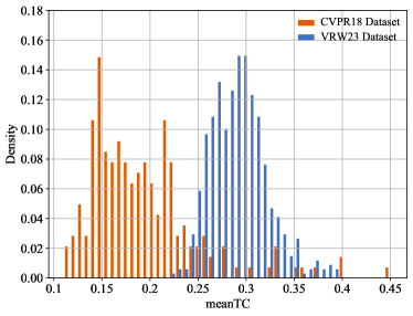
We visualize the meanTC histograms of the CVPR18 and VRW23 datasets in Fig. 4, from which we observe that scanpaths in both datasets exhibit considerable diversity, which shall be computationally modeled. Moreover, the scanpaths with longer horizons in the CVPR18 dataset (e.g., more than seconds) are even less consistent, showing the difficulty of the long-term scanpath prediction.
5.2 Experimental Setups
In the main experiments, we inherit the same sampling rate in previous studies [13, 11] to downsample both the video (and the corresponding) scanpaths to five frames (and viewpoints) per second. We use one second as the context window size to create the visual and path history (i.e., ), and produce one-second future scanpath (i.e., the prediction horizon ). As for predicting scanpaths that are longer than one second, we just apply our PID controller-based sampling strategy multiple rounds, as described in Sec. 4.
We set the quantization step size in Eq. (4) to (with a quantization error ). The resolution of the extracted viewport is set to , covering an FoV of . As shown in Fig. 3, for the historical visual context, we set , , , and ; for the historical path context, we set ; for the causal patch context, we set . The number of Gaussian components in GMM in Eq. (3.3) is set to . For the PID controller, we set the sampling interval in Eq. (28) as the inverse of the sampling rate, i.e., second. The set of parameters in the PID controller to adjust the accelaration in Eq. (31) are set using the Ziegler–Nichols method [67] to , , and , respectively. For the CVPR18 dataset, we set and , while for the VRW23 dataset, we set and .
During model training, we first initialize the convolution layers in ResNet-50 for visual feature extraction with the pre-trained weights on ImageNet, and initialize the remaining parameters by He’s method [68]. We then optimize the entire method by minimizing Eq. (27) using Adam [54] with an initial learning rate of and a minibatch size of (where we parallelize data on NVIDIA A100 cards). We decay the learning rate by a factor of whenever the training plateaus. We train two separate models, one for the CVPR18 dataset by following the suggestion of the training/test set splitting in [13] and the other for the VRW23 dataset, in which we use the first videos for training and the rest videos for testing.
We evaluate panoramic video scanpath predictors from three perspectives: 1) prediction accuracy, 2) perceptual realism, and 3) generalization to unseen datasets. For prediction accuracy evaluation, we introduce two quantitative metrics: minimum orthodromic distance777The orthodromic distance is also known as the great-circle or the spherical distance. and maximum temporal correlation. Specifically, given a panoramic video, we define the set of scanpaths, , corresponding to different viewers as the ground-truths. The minimum orthodromic distance between and the set of predicted can be computed by
| (34) |
where the between two scanpaths of the same length is defined as
| (35) |
Similarly, the maximum temporal correlation between and is calculated by
| (36) |
It is noteworthy that we intentionally opt for best-case set-to-set distance metrics to avoid specifying, for each predicted scanpath from , one ground-truth from . Moreover, such distances have the advantage over path-to-path distances in terms of quantifying the prediction accuracy without penalizing the generation diversity.
| Model | - | - | - | - | - | - | ||
|---|---|---|---|---|---|---|---|---|
| Path-Only | ||||||||
| Nguyen18 (CB-sal) | ||||||||
| Nguyen18 (GT-sal) | ||||||||
| Xu18 (CB-sal) | ||||||||
| Xu18 (GT-sal) | 0.522 | |||||||
| TRACK (CB-sal) | ||||||||
| TRACK (GT-sal) | 0.456 | 0.197 | 0.234 | 0.261 | ||||
| Ours- | 0.644 | 0.988 | 0.971 | 0.956 | ||||
| Ours- | 0.119 | 0.157 | 0.190 | 0.708 | 0.993 | 0.981 | 0.971 |
| Model | - | - | - | - | - | - | ||
|---|---|---|---|---|---|---|---|---|
| Path-Only | ||||||||
| Nguyen18 (CB-sal) | ||||||||
| Nguyen18 (GT-sal) | ||||||||
| Xu18 (CB-sal) | ||||||||
| Xu18 (GT-sal) | ||||||||
| TRACK (CB-sal) | ||||||||
| TRACK (GT-sal) | ||||||||
| Ours- | 0.645 | 0.171 | 0.241 | 0.296 | 0.738 | 0.989 | 0.966 | 0.940 |
| Ours- | 0.542 | 0.118 | 0.177 | 0.226 | 0.796 | 0.995 | 0.981 | 0.965 |
Additionally, inspired by the time-delay embedding technique in dynamical systems [69, 70], we introduce the sliced versions of the minimum orthodromic distance and the maximum temporal correlation, respectively. We first slice each ground-truth scanpath , for , into overlapping sub-paths of length , , in which the overlap between two consecutive sub-paths is set to . This gives rise to sets of sliced scanpaths , where . Similarly, for the predicted scanpath set , we create sets of sliced scanpaths , where , and compute the sliced minimum orthodromic distance and the sliced maximum temporal correlation by
| (37) |
and
| (38) |
respectively. In the experiments, is set to , corresponding to one-second, two-second, and three-second sliced scanpaths, respectively. We will append the corresponding number to the evaluate metric (e.g., -) to differentiate the three different settings. After determining , can be set accordingly. Generally, the OD metric family focuses more on the pointwise local comparison, while the TC metric family emphasizes more on global covariance measurement.

(a)

(b)

(c)

(d)
For perceptual realism evaluation, we first train a separate classifier for each scanpath predictor to discriminate its predicted scanpaths from those generated by humans. The underlying idea is conceptually similar to that in GANs [71], except that we perform post hoc training of the classifier as the discriminator. A higher classification accuracy indicates poorer perceptual realism. Rather than solely relying on machine discrimination, we also perform a formal psychophysical experiment to quantify the perceptual realism of scanpaths. We reserve the details on how to train the classifiers and how to perform the psychophysical experiment in later subsections.
5.3 Main Experiments
5.3.1 Prediction Accuracy Results
We compare the proposed method with several panoramic scanpath predictors, including a path-only seq2seq model [11], Nguyen18 [14], Xu18 [13], and TRACK [11]. Nguyen18, Xu18, and TRACK rely on external saliency models for scanpath prediction. We follow the experimental setting in [11], and exploit two types of saliency maps. The first type is the content-based saliency map produced by a panoramic saliency model [14], denoted by CB-sal. The second type is the ground-truth saliency map aggregated spatiotemporally from multiple human viewers, denoted by GT-sal. Nevertheless, we point out two caveats when using ground-truth saliency maps. First, future scanpaths may be unavoidable to participate in the computation of the saliency map at the current time stamp. Second, the saliency prediction module is ahead of the scanpath prediction module for some competing methods such as TRACK [11]. Both cases violate the causal assumption in scanpath prediction if the ground-truth saliency map is exploited.
We re-train all competing models, following the respective training procedures. The prediction horizon for the path-only model, Nguyen18, Xu18, and TRACK during training is set to , , , and , respectively. All competing methods are deterministic, producing a single scanpath for each test panoramic video (i.e., in Eqs. (34), (36), (37) and (38)). In stark contrast, our method is designed to be probabilistic as a natural way of capturing the uncertainty and diversity of scanpaths. Thus, we report the results of two variants of the proposed method, one samples scanpaths for each test video (i.e., ), denoted by Ours-, and the other samples scanpaths (i.e., ), denoted by Ours-.

(a)

(b)

(c)

(d)
We report the , , , and results of all methods on the CVPR18 dataset in Table III and on the VRW23 dataset in Table IV, respectively. The prediction horizon is set to (corresponding to a 30-second scanpath) for CVPR18 dataset and (corresponding to a 10-second scanpath) for VRW23 dataset. The slice length, , for computing and is set to one of the three values, . From the tables, we make several interesting observations. First, the path-only model provides a highly nontrivial solution to panoramic scanpath prediction, consistent with the observation in [11]. This also explains the emerging but possibly “biased” view that the historical scanpath is all you need [45]. In particular, the path-only model performs better (or at least on par with) Xu18 (CB sal) and TRACK (CB sal) under the OD metric family. Second, the performance of saliency-based scanpath predictors improve when the ground-truth saliency maps are allowed on the CVPR18 dataset. This provides evidence that in our experimental setting, the (historical) visual context can be beneficial, if it is extracted and incorporated properly. Nevertheless, such visual information may be less useful when the prediction horizon is relatively short, or even harmful with inapt incorporation, as evidenced by the temporal correlation results on the VRW23 dataset. Third, the proposed methods provide consistent performance improvements on both datasets and under all evaluation metrics (except for on the CVPR18 dataset).
We take a closer look at the performance variations of scanpath predictors by varying the prediction horizon in the unit of second. Figs. 5 and 6 show the results under , , -, and - on the CVPR18 and VRW23 datasets, respectively. We find that initially our methods underperform slightly but quickly catch up and significantly outperform the competing methods in the long run. This makes sense because deterministic methods are typically optimized for pointwise distance losses, and thus perform more accurately at the beginning with highly consistent viewpoints. As the prediction horizon increases, different viewers tend to explore the panoramic virtual scene in rather different ways, leading to diverse scanpaths that cause deterministic methods to degrade. Meanwhile, we also make a similar “counterintuitive” observation: models with predicted saliency show noticeably better temporal correlation but poorer orthodromic distance than those with ground-truth saliency on the VRW23 dataset (not on the CVPR18 dataset). We believe these may arise because of the interplay of the differences in dataset characteristics (e.g., the duration of panoramic videos) and in metric emphasis (i.e., local pointwise versus global listwise comparison). In addition, our methods are fairly stable under sliced metrics.
5.3.2 Perceptual Realism Results
Machine Discrimination. Apart from prediction accuracy, we also evaluate the perceptual realism of the predicted scanpaths. We first take a machine discrimination approach: train DNN-based binary classifiers to discriminate whether input viewport sequences are real (i.e., sampled along human scanpaths) or fake (i.e., sampled along machine-predicted scanpaths). As shown in Fig. 7, we adopt a variant of ResNet-50 (the same as used in Sec. 3.2.1) to extract the visual features from input viewport sequences with frames, leading to the intermediate representation of size . We then reshape it to , and process the representation with four residual blocks and a back-end FC layer to produce an output representation of size . Inspired by the multi-head attention in [51], our residual block consists of a front-end FC layer, a transposing operation, a 2D convolution with a kernel size of , a second transposing operation, and a back-end FC layer with a skip connection. After the front-end FC layer, we split the representation into parts, with the size of , which is transposed to . We then apply 2D convolution, and transpose the convolved representation back to . We further process it with the back-end FC layer to generate the output of size , which is added to the input as the final feature representation. Last, we take the average of the output features along the time dimension, and add a sigmoid activation to estimate the probabilities.
| Model | CVPR18 Dataset | VRW23 Dataset | ||||
|---|---|---|---|---|---|---|
| Path-Only | ||||||
| Nguyen18 (CB-sal) | ||||||
| Nguyen18 (GT-sal) | ||||||
| Xu18 (CB-sal) | ||||||
| Xu18 (GT-sal) | ||||||
| TRACK (CB-sal) | ||||||
| TRACK (GT-sal) | ||||||
| Ours- | 0.949 | 0.854 | 0.144 | 0.868 | 0.597 | 0.329 |
We train the classifiers to minimize the cross-entropy loss, following the training procedures described in Sec. 5.2. We test the classifiers using the classification accuracy, the score, and the cross-entropy objective. It is clear from Table V that, our method outperforms the others on both datasets. Moreover, all methods have better results on the VRW23 dataset, which is attributed to the overall shorter video durations. After all, the longer you predict, the more possible mistakes you would make, which are easier spotted by the classifiers.
| Model | CVPR18-Trained | VRW23-Trained | ||||||
|---|---|---|---|---|---|---|---|---|
| - | - | - | - | |||||
| Path-Only | ||||||||
| TRACK (CB-sal) | ||||||||
| TRACK (GT-sal) | ||||||||
| Ours- | 0.416 | 0.141 | 0.882 | 0.996 | 0.435 | 0.148 | 0.887 | 0.997 |
| Ours- | 0.322 | 0.093 | 0.919 | 0.998 | 0.344 | 0.098 | 0.923 | 0.998 |
| Model | CVPR18-Trained | VRW23-Trained | ||||||
| - | - | - | - | |||||
| Path-Only | 0.125 | 0.064 | 0.593 | 0.353 | 0.729 | |||
| TRACK (CB-sal) | ||||||||
| TRACK (GT-sal) | 0.174 | 0.068 | ||||||
| Ours- | 0.801 | 0.994 | 0.996 | |||||
| Ours- | 0.898 | 0.999 | 0.564 | 0.211 | 0.747 | 0.999 | ||
Psychophysical Experiment. We next take a psychophysical approach: invite human subjects to judge whether the viewed viewport sequences are real or not. We select and panoramic videos from the CVPR18 and VRW23 test sets, respectively. For each test video, we generate viewport sequences by sampling along different scanpaths produced by the path-only model, Xu18 (CB-sal), Xu18 (GT-sal), TRACK (CB-sal), TRACK (GT-sal), the proposed method, and one human viewer (as the real instance). Fig. 8 shows the graphical user interface customized for this experiment. All viewport videos are shown in the actual resolution of , with a framerate of fps888We upconvert the framerate from the default fps to fps using spherical linear interpolation [72]. and in a randomized temporal order. The “Real” and “Fake” bottoms are utilized to collect the perceptual realism judgment for each video, both of which serve as the “Next” bottom for the next video playback. Each video can be replayed multiple times until the subject is confident with her/his rating, but we encourage her/him to make the judgment at the earliest convenience. We also allow the subject to go back to the previous video with the “Back” bottom in case s/he would like to change the rating for some reason, as a way of mitigating the serial dependence between adjacent videos [73]. For each viewport sequence, we gather human data from subjects with normal and correct-to-normal visual acuity. They have general knowledge of image processing and computer vision, but do not know the detailed purpose of the study. We include a training session to familiarize them with the user interface and the moving patterns of real viewport sequences. Each subject is asked to give judgments to all viewport sequences.


The perceptual realism of each model is defined as the number of viewport sequences labeled as real divided by the total number of sequences corresponding to that model. As shown in Fig. 9, the perceptual realism of scanpaths by our model is very close to the ground-truth scanpaths, and is much better than scanpaths by the competing methods on both datasets. This is due primarily to the accurate probabilistic modeling of the uncertainty and diversity of scanpaths and the PID controller-based sampler that takes into account Newton’s laws of motion during sampling. It is also interesting to note that TRACK (CB-sal) ranks third in the psychophysical experiment, which is consistent with the results in Fig. 5 (d) and Fig. 6 (d). This indicates the TC metric family is more in line with human visual perception.
From a qualitative perspective, we find that the deterministic saliency-based methods are easier to swing between two objects when there are multiple salient objects in the scene. Meanwhile, Xu18 exhibits a tendency to remain fixated on one position. This phenomenon may be attributed to the original model design for short-term scanpath prediction. As delineated in [11], the past scanpath suffices to serve as the historical context for short-term prediction. Consequently, it is likely that when the initial viewpoints are situated on some objects, it is easy for Xu18 to get trapped in such bad “local optima.” On the contrary, our method does not suffer from any of the above problems.
5.3.3 Cross-Dataset Generalization Results
To test the generalizability of CVPR18-trained and VRW23-trained models, we conduct cross-dataset experiments on two relatively smaller datasets - MMSys18 [65] and PAMI19 [42]. Tables VI and VII show the results, in which we omit Nguyen18 and Xu18 as they are inferior to the path-only and TRACK models. Consistent with the results in the main experiments, our methods outperform the others on both datasets in terms of temporal correlation metrics (except for Ours- trained on VRW23 and tested on PAMI19). For the orthodromic distance metrics, our methods achieve the best results on MMSys18, but are worse than the path-only method on PAMI19. Interestingly, the path-only model always performs better than TRACK. Moreover, our methods trained on CVPR18 have better performance than those trained on VRW23 when tested on PAMI19, while both perform similarly when tested on MMSys18. This implies that the scanpath distribution of PAMI19 is closer to that of CVPR18.
5.4 Ablation Experiments
| Model | CVPR18 Dataset | VRW23 Dataset | ||||||
|---|---|---|---|---|---|---|---|---|
| Random | Max | Beam Search | PID Controller | Random | Max | Beam Search | PID Controller | |
| Visual | ||||||||
| Visual + H-Path | ||||||||
| Visual + H-Path + C-Path | ||||||||
| Representation | CVPR18 Dataset | VRW23 Dataset |
|---|---|---|
| Spherical | ||
| 3D Eculidean | ||
| Relative |
We conduct a series of ablation experiments to justify the rationality of our model design. For experiments that need no scanpath sampling, we report the expected code length in Eq. (27). As for experiments that require scanpath sampling, we set the prediction horizon , sample scanpaths (i.e., ), and report the results.
Input Component. We first probe the contribution of the three input components in our model, i.e., the historical visual context, the historical path context, and the causal path context, by training three variants: 1) the model with only the historical visual context, 2) the model with the historical visual and path contexts, and 3) the full model with all three input components. We report the results in Table VIII (see the PID Controller columns). Our results show that adding the historical path context clearly increases the maximum temporal correlation, particularly on VRW23. Moreover, the causal path context also contributes substantially, validating its effectiveness as an autoregressive prior.
Scanpath Representation. We next probe different scanpath representations: 1) spherical coordinates , 2) 3D Euclidean coordinates , and 3) relative coordinates . Table IX reports the expected code length results, in which we find that our relative representation performs the best, followed by the 3D Euclidean coordinates.
Quantization Step Size. We further study the effect of the quantization step size on the probabilistic modeling of our method. Specifically, we test four different quantization step sizes of , which, respectively, correspond to the largest quantization errors of . We report the results in Fig. 10, from which we find that a proper quantization step size is crucial to the final scanpath prediction performance. A very large quantization step size would induce a noticeable quantization error, which impairs the diversity modeling. Conversely, a very small quantization step size would hinder the training of smooth entropy models. This provides strong justification for the use of the discretized probability model (in Eq. (26)) over its continuous counterpart (in Eq. (3.3)).
Sampler. We last compare our PID controller-based sampler to three counterparts: the naive random sampler, the max sampler, and the beam search sampler (with a beam width of ). Table VIII shows the results. Our PID controller-based sampler outperforms all three competing samplers by a large margin for the three model variants and on the two datasets. We also observe that the causal path context increases the performance of the random sampler and our PID controller-based sampler, but decreases the performance of the max and beam search samplers. This suggests that the causal path context is a double-edged sword: conditioning on an inaccurate causal path context would lead to degraded performance.

6 Conclusion and Discussion
We have described a new probabilistic approach to panoramic scanpath prediction from the perspective of lossy data compression. We explored a simple criterion—expected code length minimization—to train a discrete conditional probability model for quantized scanpaths. We also presented a PID controller-based sampler to generate realistic scanpaths from the learned probability model.
Our method is rooted in density estimation, the mother of all unsupervised learning problems. While the question of how to reliably assess the performance of unsupervised learning methods on finite data remains open in the general sense, we provide a quantitative measure, expected code length, in the context of scanpath prediction. We have carefully designed ablation experiments to point out the importance of the quantization step during probabilistic modeling. A similar idea that optimizes the coding rate reduction has been explored previously in image segmentation [74] and recently in representation learning [75].
We have advocated the adoption of best-case set-to-set distances to quantitatively compare the set of predicted scanpaths to the set of human scanpaths. Our set-to-set distances can be easily generalized by first finding an optimal bipartite matching between predicted and ground truth scanpaths (for example, using the Hungarian algorithm [76]), and then comparing pairs of matched scanpaths. We have experimented with this variant of set-to-set distances, and arrive at similar conclusions in Sec. 5.3.
One goal of scanpath prediction is to model and understand how humans explore different panoramic virtual scenes. Thus, we have emphasized on testing the perceptual realism of predicted scanpaths via machine discrimination and human verification. Although it is relatively easy for the trained classifiers to identify predicted scanpaths, our method performs favorably in “fooling” human subjects, with a matched perceptual realism level to human scanpaths. Thus, our method appears promising for a number of panoramic video processing applications, including panoramic video compression [58], streaming [43], and quality assessment [66].
Finally, we have introduced a relative representation of scanpaths in the viewport domain. This scanpath representation is well aligned with the viewport sequence, and simplifies the computational modeling of panoramic videos, and transforms the panoramic scanpath prediction problem to a planar one. We believe our relative representation has great potential in a broader 360° computer vision tasks, including panoramic video semantic segmentation, object detection, and object tracking.
References
- [1] D. Noton and L. Stark, “Scanpaths in saccadic eye movements while viewing and recognizing patterns,” Vision Research, vol. 11, no. 9, pp. 929–942, 1971.
- [2] ——, “Scanpaths in eye movements during pattern perception,” Science, vol. 171, no. 3968, pp. 308–311, 1971.
- [3] F. Perazzi, A. Sorkine-Hornung, H. Zimmer, P. Kaufmann, O. Wang, S. Watson, and M. Gross, “Panoramic video from unstructured camera arrays,” Computer Graphics Forum, vol. 34, no. 2, pp. 57–68, 2015.
- [4] G. Zoric, L. Barkhuus, A. Engström, and E. Önnevall, “Panoramic video: Design challenges and implications for content interaction,” in European Conference on Interactive TV and Video, 2013, pp. 153–162.
- [5] K.-T. Ng, S.-C. Chan, and H.-Y. Shum, “Data compression and transmission aspects of panoramic videos,” IEEE Transactions on Circuits and Systems for Video Technology, vol. 15, no. 1, pp. 82–95, 2005.
- [6] Y. Cai, X. Li, Y. Wang, and R. Wang, “An overview of panoramic video projection schemes in the IEEE 1857.9 standard for immersive visual content coding,” IEEE Transactions on Circuits and Systems for Video Technology, vol. 32, no. 9, pp. 6400–6413, 2022.
- [7] M. Xu, C. Li, Y. Liu, X. Deng, and J. Lu, “A subjective visual quality assessment method of panoramic videos,” in IEEE International Conference on Multimedia and Expo, 2017, pp. 517–522.
- [8] V. Sitzmann, A. Serrano, A. Pavel, M. Agrawala, D. Gutierrez, B. Masia, and G. Wetzstein, “Saliency in VR: How do people explore virtual environments?” IEEE Transactions on Visualization and Computer Graphics, vol. 24, no. 4, pp. 1633–1642, 2018.
- [9] T. Rhee, L. Petikam, B. Allen, and A. Chalmers, “MR360: Mixed reality rendering for 360° panoramic videos,” IEEE Transactions on Visualization and Computer Graphics, vol. 23, no. 4, pp. 1379–1388, 2017.
- [10] W.-T. Lee, H.-I. Chen, M.-S. Chen, I.-C. Shen, and B.-Y. Chen, “High-resolution 360 video foveated stitching for real-time VR,” Computer Graphics Forum, vol. 36, no. 7, pp. 115–123, 2017.
- [11] M. F. R. Rondón, L. Sassatelli, R. Aparicio-Pardo, and F. Precioso, “TRACK: A new method from a re-examination of deep architectures for head motion prediction in 360° videos,” IEEE Transactions on Pattern Analysis and Machine Intelligence, vol. 44, no. 9, pp. 5681–5699, 2022.
- [12] C.-L. Fan, J. Lee, W.-C. Lo, C.-Y. Huang, K.-T. Chen, and C.-H. Hsu, “Fixation prediction for 360° video streaming in head-mounted virtual reality,” in Workshop on Network and Operating Systems Support for Digital Audio and Video, 2017, pp. 67–72.
- [13] Y. Xu, Y. Dong, J. Wu, Z. Sun, Z. Shi, J. Yu, and S. Gao, “Gaze prediction in dynamic 360° immersive videos,” in IEEE Conference on Computer Vision and Pattern Recognition, 2018, pp. 5333–5342.
- [14] A. Nguyen, Z. Yan, and K. Nahrstedt, “Your attention is unique: Detecting 360-degree video saliency in head-mounted display for head movement prediction,” in ACM International Conference on Multimedia, 2018, pp. 1190–1198.
- [15] Y. Xu, Z. Zhang, and S. Gao, “Spherical DNNs and their applications in 360° images and videos,” IEEE Transactions on Pattern Analysis and Machine Intelligence, vol. 44, no. 10, pp. 7235–7252, 2022.
- [16] Y. Li, Y. Xu, S. Xie, L. Ma, and J. Sun, “Two-layer FOV prediction model for viewport dependent streaming of 360-degree videos,” in International Conference on Communications and Networking in China, 2018, pp. 501–509.
- [17] W. Sun, Z. Chen, and F. Wu, “Visual scanpath prediction using IOR-ROI recurrent mixture density network,” IEEE Transactions on Pattern Analysis and Machine Intelligence, vol. 43, no. 6, pp. 2101–2118, 2021.
- [18] M. Assens, X. Giro-i Nieto, K. McGuinness, and N. E. O’Connor, “PathGAN: Visual scanpath prediction with generative adversarial networks,” in European Conference on Computer Vision Workshops, 2018, pp. 406–422.
- [19] D. Martin, A. Serrano, A. W. Bergman, G. Wetzstein, and B. Masia, “ScanGAN360: A generative model of realistic scanpaths for 360° images,” IEEE Transactions on Visualization and Computer Graphics, vol. 28, no. 5, pp. 2003–2013, 2022.
- [20] T. Cover and J. Thomas, Elements of Information Theory. Wiley, 2012.
- [21] T. Baltrušaitis, C. Ahuja, and L.-P. Morency, “Multimodal machine learning: A survey and taxonomy,” IEEE Transactions on Pattern Analysis and Machine Intelligence, vol. 41, no. 2, pp. 423–443, 2018.
- [22] R. Bellman, Adaptive Control Processes: A Guided Tour. Princeton University Press, 2015.
- [23] T. Ngo and B. Manjunath, “Saccade gaze prediction using a recurrent neural network,” in IEEE International Conference on Image Processing, 2017, pp. 3435–3439.
- [24] C. Wloka, I. Kotseruba, and J. K. Tsotsos, “Active fixation control to predict saccade sequences,” in IEEE Conference on Computer Vision and Pattern Recognition, 2018, pp. 3184–3193.
- [25] C. Xia, J. Han, F. Qi, and G. Shi, “Predicting human saccadic scanpaths based on iterative representation learning,” IEEE Transactions on Image Processing, vol. 28, no. 7, pp. 3502–3515, 2019.
- [26] R. Klein, “Inhibitory tagging system facilitates visual search,” Nature, vol. 334, no. 6181, pp. 430–431, 1988.
- [27] R. A. J. de Belen, T. Bednarz, and A. Sowmya, “ScanpathNet: A recurrent mixture density network for scanpath prediction,” in IEEE Conference on Computer Vision and Pattern Recognition Workshops, 2022, pp. 5010–5020.
- [28] J. M. Wolfe, “Guided search 6.0: An updated model of visual search,” Psychonomic Bulletin & Review, vol. 28, no. 4, pp. 1060–1092, 2021.
- [29] N. D. B. Bruce and J. K. Tsotsos, “Saliency, attention, and visual search: An information theoretic approach,” Journal of Vision, vol. 9, no. 3, pp. 1–24, 2009.
- [30] X. Huang, C. Shen, X. Boix, and Q. Zhao, “SALICON: Reducing the semantic gap in saliency prediction by adapting deep neural networks,” in IEEE International Conference on Computer Vision, 2015, pp. 262–270.
- [31] K. He, G. Gkioxari, P. Dollar, and R. Girshick, “Mask R-CNN,” in IEEE International Conference on Computer Vision, 2017, pp. 2961–2969.
- [32] M. Assens, X. Giro-i Nieto, K. McGuinness, and N. E. O’Connor, “SaltiNet: Scan-path prediction on 360 degree images using saliency volumes,” in IEEE International Conference on Computer Vision Workshops, 2017, pp. 2331–2338.
- [33] Y. Zhu, G. Zhai, and X. Min, “The prediction of head and eye movement for 360 degree images,” Signal Processing: Image Communication, vol. 69, pp. 15–25, 2018.
- [34] P. F. Felzenszwalb, R. B. Girshick, D. McAllester, and D. Ramanan, “Object detection with discriminatively trained part-based models,” IEEE Transactions on Pattern Analysis and Machine Intelligence, vol. 32, no. 9, pp. 1627–1645, 2010.
- [35] M. A. Kerkouri, M. Tliba, A. Chetouani, and M. Sayeh, “SalyPath360: Saliency and scanpath prediction framework for omnidirectional images,” in Electronic Imaging Symposium, 2022, pp. 168–1 – 168–7.
- [36] Y. Dahou, M. Tliba, K. McGuinness, and N. O’Connor, “ATSal: An attention based architecture for saliency prediction in 360° videos,” in International Conference on Pattern Recognition Workshops, 2020, pp. 305–320.
- [37] M. Cornia, L. Baraldi, G. Serra, and R. Cucchiara, “A deep multi-level network for saliency prediction,” in International Conference on Pattern Recognition, 2016, pp. 3488–3493.
- [38] B. D. Lucas and T. Kanade, “An iterative image registration technique with an application to stereo vision,” in International Joint Conference on Artificial Intelligence, 1981, pp. 674–679.
- [39] A. De Abreu, C. Ozcinar, and A. Smolic, “Look around you: Saliency maps for omnidirectional images in VR applications,” in International Conference on Quality of Multimedia Experience, 2017, pp. 1–6.
- [40] J. Pan, E. Sayrol, X. Giro-i Nieto, K. McGuinness, and N. E. O’Connor, “Shallow and deep convolutional networks for saliency prediction,” in IEEE Conference on Computer Vision and Pattern Recognition, 2016, pp. 598–606.
- [41] E. Ilg, N. Mayer, T. Saikia, M. Keuper, A. Dosovitskiy, and T. Brox, “FlowNet 2.0: Evolution of optical flow estimation with deep networks,” in IEEE Conference on Computer Vision and Pattern Recognition, 2017, pp. 2462–2470.
- [42] M. Xu, Y. Song, J. Wang, M. Qiao, L. Huo, and Z. Wang, “Predicting head movement in panoramic video: A deep reinforcement learning approach,” IEEE Transactions on Pattern Analysis and Machine Intelligence, vol. 41, no. 11, pp. 2693–2708, 2019.
- [43] C. Li, W. Zhang, Y. Liu, and Y. Wang, “Very long term field of view prediction for 360-degree video streaming,” in IEEE Conference on Multimedia Information Processing and Retrieval, 2019, pp. 297–302.
- [44] M. Cornia, L. Baraldi, G. Serra, and R. Cucchiara, “Predicting human eye fixations via an LSTM-based saliency attentive model,” IEEE Transactions on Image Processing, vol. 27, no. 10, pp. 5142–5154, 2018.
- [45] F.-Y. Chao, C. Ozcinar, and A. Smolic, “Transformer-based long-term viewport prediction in 360° video: Scanpath is all you need,” in IEEE International Workshop on Multimedia Signal Processing, 2021, pp. 1–6.
- [46] M. Müller, Information Retrieval for Music and Motion. Springer Berlin Heidelberg, 2007.
- [47] T. S. Cohen, M. Geiger, J. Köhler, and M. Welling, “Spherical CNNs,” in International Conference on Learning Representations, 2018.
- [48] C. Esteves, C. Allen-Blanchette, A. Makadia, and K. Daniilidis, “Learning SO(3) equivariant representations with spherical CNNs,” in European Conference on Computer Vision, 2018, pp. 52–68.
- [49] C. Jiang, J. Huang, K. Kashinath, Prabhat, P. Marcus, and M. Niessner, “Spherical CNNs on unstructured grids,” in International Conference on Learning Representations, 2019.
- [50] C. Wu, R. Zhang, Z. Wang, and L. Sun, “A spherical convolution approach for learning long term viewport prediction in 360 immersive video,” in AAAI Conference on Artificial Intelligence, 2020, pp. 14 003–14 040.
- [51] A. Vaswani, N. Shazeer, N. Parmar, J. Uszkoreit, L. Jones, A. N. Gomez, L. u. Kaiser, and I. Polosukhin, “Attention is all you need,” in Advances in Neural Information Processing Systems, 2017.
- [52] J. Devlin, M.-W. Chang, K. Lee, and K. Toutanova, “BERT: Pre-training of deep bidirectional transformers for language understanding,” in Annual Conference of the North American Chapter of the Association for Computational Linguistics: Human Language Technologies, 2019.
- [53] E. P. Simoncelli, “Distributed representation and analysis of visual motion,” Ph.D. dissertation, Massachusetts Institute of Technology, 1993.
- [54] D. Kingma and J. Ba, “Adam: A method for stochastic optimization,” in International Conference for Learning Representations, 2015.
- [55] C. M. Bishop and N. M. Nasrabadi, Pattern Recognition and Machine Learning. Springer, 2006.
- [56] J. Ballé, V. Laparra, and E. P. Simoncelli, “End-to-end optimized image compression,” in International Conference on Learning Representations, 2016.
- [57] M. Li, K. Ma, J. You, D. Zhang, and W. Zuo, “Efficient and effective context-based convolutional entropy modeling for image compression,” IEEE Transactions on Image Processing, vol. 29, pp. 5900–5911, 2020.
- [58] M. Li, K. Ma, J. Li, and D. Zhang, “Pseudocylindrical convolutions for learned omnidirectional image compression,” arXiv preprint arXiv:2112.13227, 2021.
- [59] X. Sui, K. Ma, Y. Yao, and Y. Fang, “Perceptual quality assessment of omnidirectional images as moving camera videos,” IEEE Transactions on Visualization and Computer Graphics, vol. 28, no. 8, pp. 3022–3034, 2022.
- [60] K. He, X. Zhang, S. Ren, and J. Sun, “Deep residual learning for image recognition,” in IEEE Conference on Computer Vision and Pattern Recognition, 2016, pp. 770–778.
- [61] L. Devroye, Handbooks in Operations Research and Management Science. Elsevier, 2006.
- [62] K. H. Ang, G. Chong, and Y. Li, “PID control system analysis, design, and technology,” IEEE Transactions on Control Systems Technology, vol. 13, no. 4, pp. 559–576, 2005.
- [63] Y. Bao, H. Wu, T. Zhang, A. A. Ramli, and X. Liu, “Shooting a moving target: Motion-prediction-based transmission for 360-degree videos,” in IEEE International Conference on Big Data, 2016, pp. 1161–1170.
- [64] C. Wu, Z. Tan, Z. Wang, and S. Yang, “A dataset for exploring user behaviors in VR spherical video streaming,” in ACM Multimedia Systems Conference, 2017, pp. 193–198.
- [65] E. J. David, J. Gutiérrez, A. Coutrot, M. P. Da Silva, and P. L. Callet, “A dataset of head and eye movements for 360° videos,” in ACM Multimedia Systems Conference, 2018, pp. 432–437.
- [66] Y. Fang, Y. Yao, X. Sui, and K. Ma, “Subjective quality assessment of user-generated 360° videos,” in IEEE Conference on Virtual Reality and 3D User Interfaces Abstracts and Workshops, 2023, pp. 74–83.
- [67] J. G. Ziegler and N. B. Nichols, “Optimum settings for automatic controllers,” Transactions of the American Society of Mechanical Engineers, vol. 64, no. 8, pp. 759–765, 1942.
- [68] K. He, X. Zhang, S. Ren, and J. Sun, “Delving deep into rectifiers: Surpassing human-level performance on ImageNet classification,” in IEEE Conference on Computer Vision and Pattern Recognition, 2015, pp. 1026–1034.
- [69] T. Sauer, J. A. Yorke, and M. Casdagli, “Embedology,” Journal of Statistical Physics, vol. 65, no. 3, pp. 579–616, 1991.
- [70] W. Wang, C. Chen, Y. Wang, T. Jiang, F. Fang, and Y. Yao, “Simulating human saccadic scanpaths on natural images,” in IEEE Conference on Computer Vision and Pattern Recognition, 2011, pp. 441–448.
- [71] I. Goodfellow, J. Pouget-Abadie, M. Mirza, B. Xu, D. Warde-Farley, S. Ozair, A. Courville, and Y. Bengio, “Generative adversarial networks,” Communications of the ACM, vol. 63, no. 11, pp. 139–144, 2020.
- [72] K. Shoemake, “Animating rotation with quaternion curves,” in Proceedings of the 12th annual conference on Computer graphics and interactive techniques, 1985, pp. 245–254.
- [73] J. Fischer and D. Whitney, “Serial dependence in visual perception,” Nature Neuroscience, vol. 17, no. 5, pp. 738–743, 2014.
- [74] Y. Ma, H. Derksen, W. Hong, and J. Wright, “Segmentation of multivariate mixed data via lossy data coding and compression,” IEEE Transactions on Pattern Analysis and Machine Intelligence, vol. 29, no. 9, pp. 1546–1562, 2007.
- [75] X. Dai, S. Tong, M. Li, Z. Wu, K. H. R. Chan, P. Zhai, Y. Yu, M. Psenka, X. Yuan, and H. Y. Shum, “CTRL: Closed-loop transcription to an LDR via minimaxing rate reduction,” Entropy, vol. 24, no. 4, p. 456, 2022.
- [76] H. W. Kuhn, “The Hungarian method for the assignment problem,” Naval Research Logistics Quarterly, vol. 2, no. 1-2, pp. 83–97, 1955.