Scaling relations for finite-time first-order phase transition
Abstract
The theory of equilibrium phase transition, which traditionally does not involve time evolution, concerns only static quantities. In recent decades, owing to the development of nonequilibrium thermodynamics, there is a growing interest in nonequilibrium phase transition which concerns time evolution. It is well-known that in the absence of phase transitions, the excess work resulted from finite-rate quench is proportional to the quench rate . The time evolution in a second-order phase transition can be understood via the Kibble-Zurek mechanism, and the scaling of work is related to the critical exponents. Nevertheless, the finite-time nonequilibrium thermodynamics of the first-order phase transition remains largely unexplored. We investigate the scaling relations of some thermodynamic quantities with the quench rate in the first-order phase transition. It is shown that the excess work scales as for small quench rate. Moreover, the delay time and the transition time scale as . Our study deepens the understanding about the nonequilibrium thermodynamics of the first-order phase transition.
Introduction.–Phase transition, traditionally lying in the framework of equilibrium statistical mechanics, is primarily concerned with static quantities. Equilibrium phase transitions are drastic changes of a system’s equilibrium state under quasi-static variation of the external parameters (Callen and Griffiths, 1987; Goldenfeld, 1992). At a phase transition, a system undergoes a nonanalytic change of its properties, for example the density in a temperature-driven liquid-gas transition, or the magnetization in a paramagnet-ferromagnet transition (Chaikin and Lubensky, 1995; Imparato and Peliti, 2007). These are static properties with respect to the external parameters. In the past few decades, owing to the recent development of nonequilibrium thermodynamics (Graham and Tél, 1984; Keizer, 1987; Imparato and Peliti, 2007; Seifert, 2012; Sagawa, 2014; Bertini et al., 2015; Pineda and Stamatakis, 2018; Peliti and Pigolotti, 2021), there is a growing interest in the field of stochastic thermodynamics with phase transitions (Derrida, 1987; Garrahan et al., 2007; Mehl et al., 2008; Lacoste et al., 2008; Jack and Sollich, 2010; Ge and Qian, 2010; Herpich et al., 2018; Nyawo and Touchette, 2018; Byrd et al., 2019; Noa et al., 2019; Fei et al., 2020; Vroylandt et al., 2020; Proesmans et al., 2020a; Nguyen and Seifert, 2020; Meibohm and Esposito, 2022). A central concept in thermodynamics is the work performed on such a system (Speck and Seifert, 2004, 2005; Blickle et al., 2006; Quan et al., 2008; Engel, 2009; Nickelsen and Engel, 2011; Ryabov et al., 2013), when some external parameters of the system are varied with time. The second law of thermodynamics constrains that the work performed on the system is no less than the free energy difference between the initial and the final states. In other words, the excess work done in a finite-rate quench with respect to the quasi-static quench process is non-negative . A natural question is how thermodynamic quantities such as the excess work scale with the rate of quench.
In the regular cases without phase transitions, it is well-known that in slow isothermal processes, the excess work is proportional to the quench rate as a result of the linear response theory (Salamon and Berry, 1983; Mazonka and Jarzynski, 1999; Crooks, 2007; Scandi and Perarnau-Llobet, 2019; Ma et al., 2020; Chen et al., 2021). While in slow adiabatic processes, the excess work is proportional to the square of the quench rate according to the adiabatic perturbation theory (Sun, 1988; Polkovnikov, 2005; Rigolin et al., 2008; De Grandi and Polkovnikov, 2010; Polkovnikov et al., 2011; Chen et al., 2019). However, in the presence of phase transitions, the scaling behavior becomes much more involved. For the second-order phase transition, it is found that the excess work done during a quench across the critical point exhibits power-law behavior with the quench rate and the corresponding exponents are fully determined by the dimension of the system and the critical exponents of the transition (Fei et al., 2020; Zhang and Quan, 2022), as in the traditional Kibble-Zurek mechanism (Kibble, 1976, 1980; Zurek, 1985, 1996; del Campo, 2018; Cui et al., 2020). Besides the second-order phase transition, the first-order phase transition is ubiquitous in nature, e.g., in biochemical (Ge and Qian, 2009, 2010; Qian et al., 2016; Pineda and Stamatakis, 2018; Nguyen and Seifert, 2020), ecological (Li et al., 2019) and electronic systems (Freitas et al., 2022). Examples include the coil-globule transition in the process of protein folding (Anfinsen, 1972; Kaiser, 1978; Qian et al., 2016) and the information erasure in electronic devices (Koller and Athas, 1992; Hanninen and Takala, 2010; Bérut et al., 2012; Proesmans et al., 2020b). However, the scaling behavior of the excess work during a finite-time first-order phase transition has not been explored so far.
In this Letter, we study the scaling behavior of the excess work with the quench rate in the first-order phase transition. Using the mean-field Curie-Weiss model with a varying magnetic field as a paradigmatic example (Fernández et al., 2012; Collet and Formentin, 2019; Meibohm and Esposito, 2022), we uncover the scaling relation of the excess work with the quench rate as for small quench rates in the finite-time first-order phase transition. This replenishes our understanding about nonequilibrium thermodynamics in driven systems with phase transitions. Besides, we find that both the delay time and the transition time scale with the quench rate as . The scaling laws should be valid for a large class of systems with the first-order phase transition since they do not depend on the details of the systems, but are a manifestation of the nonlinear nature of their dynamics.
The model.–We consider the kinetic 1D mean-field Curie-Weiss model with ferromagnetic interaction introduced in Ref. (Meibohm and Esposito, 2022). The Curie-Weiss model consists of Ising spins , labeled , with the coupling strength . The system is embedded in a heat reservoir at an inverse temperature , and subject to a varying field controlled by some external agent. The state of the system is characterized by the magnetic moment . In the thermodynamic limit , we use the mean magnetization to denote the system state. The internal energy density is given by (Goldenfeld, 1992)
| (1) |
The deterministic dynamics is described by the equation of motion of (see Supplemental Materials (Sup, ) for details):
| (2) |
with the microscopic relaxation time .
The curve characterizing steady state as a function of is shown in Fig. 1, where we choose the parameters to be . Depending on the value of , the ordinary differential equation (2) can have one, two or three steady-state solutions. For small and large values of , the system has only one steady state ,i.e., the system is monostable. For other intermediate values of , there are three steady states: (blue line), (green line), and (orange line), i.e., the system exhibits bistability. Among the three, one is globally stable; one is metastable and the one in between is unstable. The two black dots are the turning points , where the metastability disappears.
During the quench process, the external field is tuned quasi-statically from to and the transient state of the system depends on its history. The quasi-static hysteresis loop is shown with the pink dotted curve in Fig. 1. The quasi-static state gets trapped in the local minimum as is increased quasi-statically from to , i.e., follows the lower branch even when the local minimum is metastable rather than globally stable, until the right turning point . Then the system state jumps to the upper branch. This is what we refer to as “quasi-static first-order phase transition”. So much the same for the return path. The quasi-static state remains on the upper branch and jumps down to the lower branch at the left turning point .
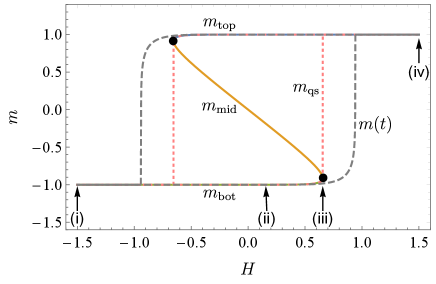
When is tuned at a finite rate , the system tries to keep pace with —but ultimately lags behind— the continually changing quasi-static state, as is shown by the gray dashed curve in Fig. 1. Although at time , the system is prepared in the equilibrium state of , i.e., , at latter times . This mismatch becomes evident around the turning point.
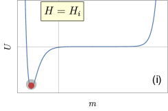
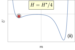
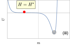
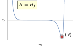
We illustrate the finite-time first-order phase transition with a particle moving in an evolving potential landscape (where satisfies ) in Fig. 2. Far away from the turning point (see Fig. 2(i-ii)), the particle is able to catch up with the change of the potential landscape and is trapped around the left local minimum, no matter whether it is globally stable or metastable. It becomes different around the turning point (see Fig. 2(iii)) where the system transitions from bistable to monostable and the left local minimum disappears. Thus the right minimum becomes the only attractor in the whole landscape. However, the evolution of the particle lags behind the drastic change of the potential. It takes some time for the particle to “feel the change of its surroundings” and make a transition to the right stable minimum. The non-catching-up obviously depends on the rate of quench. After reaching the new stable state, the particle gets stuck as the deforming of the potential landscape continues (Fig. 2(iv)).
Scaling relations of time.–During the quench process, the trajectory follows a stable local equilibrium, be it metastable or globally stable, until an abrupt transition into a totally different state from the original one. This transition relies on the system’s history and is regarded as a finite-time first-order phase transition. This is caused by the disappearance of metastability. The turning points satisfy
| (3) |
where is defined in Eq. (2). The turning points can be calculated analytically as , where
| (4) | ||||
| (5) |
Here we consider the case in which the external magnetic field is varied from the initial value to the final value according to the linear protocol
| (6) |
with the quench rate and the time duration . We label the time when reaches the right turning point as the turning time (Li et al., 2019).
It is important to note that while the potential landscape has significantly changed from bistable to monostable at the turning time , in a finite-rate quench the dynamics of the system cannot catch up with the change of the potential landscape, i.e., the system displays a delay in transitioning to the monostable state. The transition occurs later than the turning time by a delay time defined through which depends on the quench rate .
We further analyze the scaling relation between the delay time and the quench rate. We shift the variables in the following way: . The evolution equation is turned into
| (7) |
For slow quench, the equation of motion around the turning point can be approximated as (see Supplemental Materials (Sup, ) for details)
| (8) |
It can be adimensionalized into
| (9) |
by rescaling the variables
| (10) | ||||
| (11) |
where
| (12) | ||||
| (13) |
Under the asymptotic boundary condition Eq. (9) is solved in terms of the Airy function (Jung et al., 1990)
| (14) |
In this way, the delay time can be computed as
| (15) |
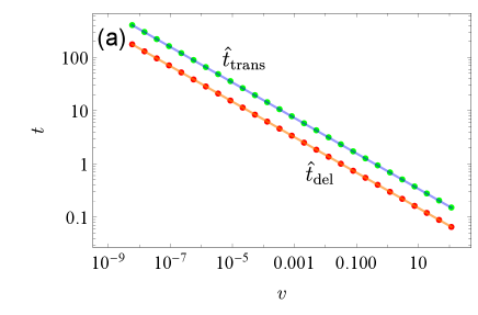
where represents the first zero point of the Airy Prime function. As is shown in Fig. 3(a), the analytical expression matches well with the numerical results.
Besides the delay time , there is another time characterizing the non-catching-up of the dynamics. When the system is quenched at a finite rate, the transition time to reach the monostable state, which is defined through depends on the quench rate . Here stands for the non-degenerate root of , with the expression
| (16) |
For , can be approximated by .
The transition time can be calculated as
| (17) |
where stands for the first zero point of the Airy function (Li et al., 2019).
Equations (15) and (17) show that both the delay time and the transition time scale with the quench rate as . The matching between analytical expressions and numerical results for and is illustrated in Fig. 3(a). The exponent 1/3 results from the quadratic leading order around the turning point in the Curie-Weiss model.
With the information about the delay time, we can estimate the time we have to save the system with phase transitions from catastrophe when the metastability disappears in economic systems and climate science (Lenton et al., 2008; Li et al., 2019). And with the transition time, we are able to estimate the time it takes to reach a new stable state from the turning point.
Scaling relation of work.–In the process of a finite-rate quench, the work performed on the system is greater than that in the quasi-static quench process. In other words, the non-catching-up in the dynamics between the transient state and the quasi-static state results in the excess work, which characterizes the irreversibility of the process. It is desirable to explore the relation between the excess work and the quench rate.
From the microscopic definition of work (Jarzynski, 1997; Sekimoto, 2010), the work performed on the system is
| (18) |
In the quasi-static isothermal process, the work equals the free energy difference between the initial and final equilibrium state
| (19) |
The excess work , defined as
| (20) |
describes the excess amount work that one has to perform when the system is quenched at a finite rate rather than quasi-statically. In a slow quench, the excess work can be approximated by the enclosed rectangular area between the dynamic and quasi-static hysteresis
| (21) |
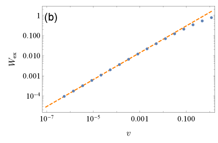
where we approximate with in the second line. From the analytical expression in Eq. (21), we obtain that the excess work scales with the quench rate as , which is verified numerically in Fig. 3(b).
Last but not least, we would like to compare our results in the first-order phase transition with the second-order phase transition and the case without phase transition in Table. 1. For finite-time isothermal processes without phase transition, the excess work due to non-quasi-static quench is proportional to the quench rate as a result of linear response theory (Salamon and Berry, 1983; Mazonka and Jarzynski, 1999; Crooks, 2007; Scandi and Perarnau-Llobet, 2019; Ma et al., 2020; Chen et al., 2021). For slow adiabatic processes, the excess work scales as according to the adiabatic perturbation theorem (Sun, 1988; Polkovnikov, 2005; Rigolin et al., 2008; De Grandi and Polkovnikov, 2010; Polkovnikov et al., 2011; Chen et al., 2019). In a second-order phase transition, the excess work performed during a quench across the critical point exhibits the scaling behavior (Fei et al., 2020; Zhang and Quan, 2022), is relevant to but different from the Kibble-Zurek scaling for the average density of defects (Kibble, 1976, 1980; Zurek, 1985, 1996). The scaling exponent is determined by the dimension of the system and the critical exponents of the transition. Here our work uncovers the scaling relation between the excess work and the quench rate in the first-order phase transition, thus replenishing our understanding for the finite-time transition. We emphasize that the scaling relation we obtain here is not restricted to the Curie-Weiss model, but should be universal for a large classs of systems with the first-order phase transition. It can also be derived from the finite-time Landau theory (Meibohm and Esposito, 2023) with a similar equation of motion of switching dynamics in bistable systems (Jung et al., 1990).
| Finite-time isothermal process (Salamon and Berry, 1983; Mazonka and Jarzynski, 1999; Crooks, 2007; Scandi and Perarnau-Llobet, 2019; Ma et al., 2020; Chen et al., 2021) | |
| Finite-time adiabatic process (Sun, 1988; Polkovnikov, 2005; Rigolin et al., 2008; De Grandi and Polkovnikov, 2010; Polkovnikov et al., 2011; Chen et al., 2019) | |
| Finite-time first-order phase transition | |
| Finite-time second-order phase transition (Fei et al., 2020; Zhang and Quan, 2022) |
Conclusions.–In this Letter, we study the time and the work applied in the quench across a first-order phase transition in the Curie-Weiss model with a varying magnetic field. We uncover a scaling relation between the excess work and the quench rate in the finite-time first-order phase transition. This replenishes our understanding about the nonequilibrium thermodynamics in driven systems with phase transitions. Moreover, we show that both the delay time and the transition time exhibit a scaling for small quench rates. The model examined here is generic, and the scaling relations should be universal for a large class of systems with the first-order phase transition. The scaling relations in Eqs. (15,17,21) do not depend on the details the models, but are a manifestation of the quadratic leading order around the turning point. This may also give us some insights into the electronic computation schemes, where non-adiabatic effects impose a tradeoff between the speed and the energy consumption that can be optimized (Bérut et al., 2012; Freitas et al., 2022).
This work is supported by the National Natural Science Foundations of China (NSFC) under Grants No. 12375028 and No. 11825501, No. 12147157.
References
- Callen and Griffiths (1987) H. B. Callen and R. B. Griffiths, American Journal of Physics 55, 860 (1987).
- Goldenfeld (1992) N. Goldenfeld, Lectures on Phase Transitions and the Renormalization Group (CRC Press, 1992).
- Chaikin and Lubensky (1995) P. M. Chaikin and T. C. Lubensky, Principles of Condensed Matter Physics, Vol. 10 (Cambridge University Press, 1995).
- Imparato and Peliti (2007) A. Imparato and L. Peliti, C. R. Phys. 8, 556 (2007).
- Graham and Tél (1984) R. Graham and T. Tél, Phys. Rev. Lett. 52, 9 (1984).
- Keizer (1987) J. Keizer, Statistical Thermodynamics of Nonequilibrium Processes (Springer New York, 1987).
- Seifert (2012) U. Seifert, Rep. Prog. Phys. 75, 126001 (2012).
- Sagawa (2014) T. Sagawa, J. Stat. Mech.: Theory Exp. 2014, P03025 (2014).
- Bertini et al. (2015) L. Bertini, A. De Sole, D. Gabrielli, G. Jona-Lasinio, and C. Landim, Rev. Mod. Phys. 87, 593 (2015).
- Pineda and Stamatakis (2018) M. Pineda and M. Stamatakis, Entropy 20, 811 (2018).
- Peliti and Pigolotti (2021) L. Peliti and S. Pigolotti, Stochastic Thermodynamics (Princeton University Press, 2021).
- Derrida (1987) B. Derrida, J. Phys. A: Math. Gen. 20, L721 (1987).
- Garrahan et al. (2007) J. P. Garrahan, R. L. Jack, V. Lecomte, E. Pitard, K. van Duijvendijk, and F. van Wijland, Phys. Rev. Lett. 98, 195702 (2007).
- Mehl et al. (2008) J. Mehl, T. Speck, and U. Seifert, Phys. Rev. E 78, 011123 (2008).
- Lacoste et al. (2008) D. Lacoste, A. W. Lau, and K. Mallick, Phys. Rev. E 78, 011915 (2008).
- Jack and Sollich (2010) R. L. Jack and P. Sollich, Prog. Theor. Phys. Supp. 184, 304 (2010).
- Ge and Qian (2010) H. Ge and H. Qian, J. R. Soc. Interface 8, 107 (2010).
- Herpich et al. (2018) T. Herpich, J. Thingna, and M. Esposito, Phys. Rev. X 8, 031056 (2018).
- Nyawo and Touchette (2018) P. T. Nyawo and H. Touchette, Phys. Rev. E 98, 052103 (2018).
- Byrd et al. (2019) T. A. Byrd, A. Erez, R. M. Vogel, C. Peterson, M. Vennettilli, G. Altan-Bonnet, and A. Mugler, Phys. Rev. E 100, 022415 (2019).
- Noa et al. (2019) C. E. F. Noa, P. E. Harunari, M. J. de Oliveira, and C. E. Fiore, Phys. Rev. E 100, 012104 (2019).
- Fei et al. (2020) Z. Fei, N. Freitas, V. Cavina, H. Quan, and M. Esposito, Phys. Rev. Lett. 124, 170603 (2020).
- Vroylandt et al. (2020) H. Vroylandt, M. Esposito, and G. Verley, Phys. Rev. Lett. 124, 250603 (2020).
- Proesmans et al. (2020a) K. Proesmans, R. Toral, and C. Van den Broeck, Physica A 552, 121934 (2020a).
- Nguyen and Seifert (2020) B. Nguyen and U. Seifert, Phys. Rev. E 102, 022101 (2020).
- Meibohm and Esposito (2022) J. Meibohm and M. Esposito, Phys. Rev. Lett. 128, 110603 (2022).
- Speck and Seifert (2004) T. Speck and U. Seifert, Phys. Rev. E 70, 066112 (2004).
- Speck and Seifert (2005) T. Speck and U. Seifert, Eur. Phys. J. B 43, 521 (2005).
- Blickle et al. (2006) V. Blickle, T. Speck, L. Helden, U. Seifert, and C. Bechinger, Phys. Rev. Lett. 96, 070603 (2006).
- Quan et al. (2008) H. T. Quan, S. Yang, and C. P. Sun, Phys. Rev. E 78, 021116 (2008).
- Engel (2009) A. Engel, Phys. Rev. E 80, 021120 (2009).
- Nickelsen and Engel (2011) D. Nickelsen and A. Engel, Eur. Phys. J. B 82, 207 (2011).
- Ryabov et al. (2013) A. Ryabov, M. Dierl, P. Chvosta, M. Einax, and P. Maass, J. Phys. A: Math. Theor. 46, 075002 (2013).
- Salamon and Berry (1983) P. Salamon and R. S. Berry, Phys. Rev. Lett. 51, 1127 (1983).
- Mazonka and Jarzynski (1999) O. Mazonka and C. Jarzynski, (1999), arXiv:cond-mat/9912121 [cond-mat.stat-mech] .
- Crooks (2007) G. E. Crooks, Phys. Rev. Lett. 99, 100602 (2007).
- Scandi and Perarnau-Llobet (2019) M. Scandi and M. Perarnau-Llobet, Quantum 3, 197 (2019).
- Ma et al. (2020) Y.-H. Ma, R.-X. Zhai, J. Chen, C. Sun, and H. Dong, Phys. Rev. Lett. 125, 210601 (2020).
- Chen et al. (2021) J.-F. Chen, C. P. Sun, and H. Dong, Phys. Rev. E 104, 034117 (2021).
- Sun (1988) C.-P. Sun, J. Phys. A: Math. Gen. 21, 1595 (1988).
- Polkovnikov (2005) A. Polkovnikov, Phys. Rev. B 72, 161201 (2005).
- Rigolin et al. (2008) G. Rigolin, G. Ortiz, and V. H. Ponce, Phys. Rev. A 78, 052508 (2008).
- De Grandi and Polkovnikov (2010) C. De Grandi and A. Polkovnikov, Quantum Quenching, Annealing and Computation (Springer Berlin Heidelberg, 2010) pp. 75–114.
- Polkovnikov et al. (2011) A. Polkovnikov, K. Sengupta, A. Silva, and M. Vengalattore, Rev. Mod. Phys. 83, 863 (2011).
- Chen et al. (2019) J.-F. Chen, C.-P. Sun, and H. Dong, Phys. Rev. E 100, 062140 (2019).
- Zhang and Quan (2022) F. Zhang and H. T. Quan, Phys. Rev. E 105, 024101 (2022).
- Kibble (1976) T. W. B. Kibble, J. Phys. A: Math. Gen. 9, 1387 (1976).
- Kibble (1980) T. Kibble, Phys. Rep. 67, 183 (1980).
- Zurek (1985) W. H. Zurek, Nature 317, 505 (1985).
- Zurek (1996) W. Zurek, Phys. Rep. 276, 177 (1996).
- del Campo (2018) A. del Campo, Phys. Rev. Lett. 121, 200601 (2018).
- Cui et al. (2020) J.-M. Cui, F. J. Gómez-Ruiz, Y.-F. Huang, C.-F. Li, G.-C. Guo, and A. del Campo, Commun. Phys. 3, 44 (2020).
- Ge and Qian (2009) H. Ge and H. Qian, Phys. Rev. Lett. 103, 148103 (2009).
- Qian et al. (2016) H. Qian, P. Ao, Y. Tu, and J. Wang, Chem. Phys. Lett. 665, 153 (2016).
- Li et al. (2019) J. H. Li, F. X.-F. Ye, H. Qian, and S. Huang, Phys. D: Nonlinear Phenom. 395, 7 (2019).
- Freitas et al. (2022) N. Freitas, K. Proesmans, and M. Esposito, Phys. Rev. E 105, 034107 (2022).
- Anfinsen (1972) C. B. Anfinsen, Biochem. J. 128, 737 (1972).
- Kaiser (1978) F. Kaiser, Zeitschrift für Naturforschung A 33, 294 (1978).
- Koller and Athas (1992) J. Koller and W. Athas, in Workshop on Physics and Computation (IEEE, 1992) pp. 267–270.
- Hanninen and Takala (2010) I. Hanninen and J. Takala, in 10th IEEE International Conference on Nanotechnology (IEEE, 2010) pp. 223–226.
- Bérut et al. (2012) A. Bérut, A. Arakelyan, A. Petrosyan, S. Ciliberto, R. Dillenschneider, and E. Lutz, Nature 483, 187 (2012).
- Proesmans et al. (2020b) K. Proesmans, J. Ehrich, and J. Bechhoefer, Phys. Rev. Lett. 125, 100602 (2020b).
- Fernández et al. (2012) R. Fernández, F. den Hollander, and J. Martínez, Commun. Math. Phys. 319, 703 (2012).
- Collet and Formentin (2019) F. Collet and M. Formentin, J. Stat. Phys. 176, 478 (2019).
- (65) .
- Jung et al. (1990) P. Jung, G. Gray, R. Roy, and P. Mandel, Phys. Rev. Lett. 65, 1873 (1990).
- Lenton et al. (2008) T. M. Lenton, H. Held, E. Kriegler, J. W. Hall, W. Lucht, S. Rahmstorf, and H. J. Schellnhuber, Proc. Natl. Acad. Sci. 105, 1786 (2008).
- Jarzynski (1997) C. Jarzynski, Phys. Rev. Lett. 78, 2690 (1997).
- Sekimoto (2010) K. Sekimoto, Stochastic Energetics, Vol. 799 (Springer Berlin Heidelberg, 2010).
- Meibohm and Esposito (2023) J. Meibohm and M. Esposito, New J. Phys. 25, 023034 (2023).