Scaling Description of Dynamical Heterogeneity and Avalanches of Relaxation in Glass-Forming Liquids
Abstract
We provide a theoretical description of dynamical heterogeneities in glass-forming liquids, based on the premise that relaxation occurs via local rearrangements coupled by elasticity. In our framework, the growth of the dynamical correlation length and of the correlation volume are controlled by a zero-temperature fixed point. We connect this critical behavior to the properties of the distribution of local energy barriers at zero temperature. Our description makes a direct connection between dynamical heterogeneities and avalanche-type relaxation associated to dynamic facilitation, allowing us to relate the size distribution of heterogeneities to their time evolution. Within an avalanche, a local region relaxes multiple times, the more the larger is the avalanche. This property, related to the nature of the zero-temperature fixed point, directly leads to decoupling of particle diffusion and relaxation time (the so-called Stokes-Einstein violation). Our most salient predictions are tested and confirmed by numerical simulations of scalar and tensorial thermal elasto-plastic models.
I Introduction
As a liquid is cooled, the relaxation time below which it acts as a solid – before displaying flow – grows from picoseconds at high temperatures up to minutes at the glass transition temperature Anderson (1995); Ediger et al. (1996); Debenedetti and Stillinger (2001); Berthier and Biroli (2011). In this regime the effective activation energy associated to grows for many liquids, leading to a super-Arrhenius behavior. Approaching , dynamics also becomes heterogeneous on a growing correlation length scale Kob et al. (1997); Yamamoto and Onuki (1998); Dalle-Ferrier et al. (2007); Karmakar et al. (2014). The underlying causes for these observations are still debated. In some views, activation is cooperative: the slowing down of the dynamics is governed by complex motion taking place on an increasingly large static length-scale. In particular, cooperativity is central in the Random First Order Theory Kirkpatrick et al. (1989); Lubchenko and Wolynes (2007); Biroli and Bouchaud (2012) and due to the growth of amorphous order. Another approach focuses on dynamical facilitation, the phenomenon by which a region’s relaxation is made much more likely by a relaxation nearby. In kinetically constrained models, such as the East model, kinetic rules induce dynamic facilitation and growth of dynamical correlations Ritort and Sollich (2003); Berthier et al. (2011). This lead to a theory Garrahan and Chandler (2002); Garrahan et al. (2007); Hedges et al. (2009) in which thermodynamics plays almost no role, but dynamics is heterogeneous (due to kinetic constraints) and the super-Arrhenius behavior is due to non-local rearrangements taking place over . Free volume Turnbull and Cohen (1961) or elastic Dyre (2006); Rainone et al. (2020); Kapteijns et al. (2021) models assume that the activation energy is not controlled by a static growing length scale: it is governed by the energy barrier of elementary rearrangements, or excitations. Recently, measurements indicated that the distribution of local energy barriers shifts to higher energy under cooling, opening up a gap at low energies where excitations are nearly absent Ciamarra et al. (2023). This shift accounts quantitatively for the dynamical slowing down of the liquid, supporting that local energy barriers may indeed control the dynamics. Yet in these views, what causes the existence of a growing length scale is unclear. An intuitive resolution of this paradox stems from the fact that on relatively short time scales, a super-cooled liquid acts as a solid Dyre (2006); Schrøder and Dyre (2020): a rearrangement corresponds to a local (plastic) strain, that affects stress away from it. Lemaitre Lemaître (2014) was the first in stressing the possible relevance of long-range stress correlations in the dynamics of super-cooled liquids, in line with various theoretical and numerical studies Chowdhury et al. (2016); Tong et al. (2020); Wu et al. (2015); Maier et al. (2017); Steffen et al. (2022); Flenner and Szamel (2015); Klochko et al. (2022). Recently, it was shown that indeed elastic interactions play an important role in dynamical facilitation Chacko et al. (2021). Moreover, Ref. Lerbinger et al. (2022) showed that heterogeneous relaxations take place in the form of plastic rearrangements that are called shear transformations Falk and Langer (1998). Following these molecular simulations studies, Ref. Ozawa and Biroli (2023) demonstrated with elasto-plastic models (traditionally used to study the plasticity of amorphous solids under loading Picard et al. (2004); Nicolas et al. (2018); Vandembroucq et al. (2004); Lin et al. (2014a); Rossi et al. (2022)) that while being controlled by local energy barriers, the dynamics can at the same time display growing dynamical correlations similar to observations in experiments and molecular simulations Berthier et al. (2005, 2011). Furthermore, such models also capture the emergence of a gap in the distribution of local barriers under cooling, which controls the dynamics Popović et al. (2021); Ozawa and Biroli (2023). We expect that the elasto-plastic description discussed above becomes more and more relevant with decreasing temperature. This paper focuses on such a lower temperature regime.
In this work we propose a scaling description of dynamical heterogeneities in glass-forming liquids, modeled as undergoing local irreversible rearrangements coupled by elasticity. We show that the dynamical correlations observed in elasto-plastic models of equilibrium glassy dynamics Ozawa and Biroli (2023) are due to ”thermal avalanches”, where rare nucleated events are followed by a pulse of faster (or facilitated) events. These avalanches are very reminiscent of the ones found in molecular simulations of super-cooled liquids Candelier et al. (2010); Keys et al. (2011); Yanagishima et al. (2017). Our analysis builds a link with systems that crackle such as disordered magnets, granular materials, and earthquakes Sethna et al. (2001); Rosso et al. (2022) even at finite temperatures Popović et al. (2021); Purrello et al. (2017); Yao and Jack (2023); Korchinski and Rottler (2022), revealing that dynamical heterogeneities are controlled by a critical point at zero temperature, with a diverging length scale and correlation volume . We provide a scaling argument expressing and in terms of the distribution of energy barriers at . Our analysis makes predictions on the power-law distribution of the size of dynamical heterogeneities, which could be tested in numerical simulations of super-cooled liquids thanks to the recent advances in the characterization of dynamical correlations Scalliet et al. (2021, 2022). Based on the properties of the zero-temperature fixed point governing thermal avalanches, we also show that the decoupling between particle diffusion and relaxation time (the so-called Stoke-Einstein violation— Tarjus and Kivelson (1995); Ediger (2000); Sengupta et al. (2013); Charbonneau et al. (2014); Kawasaki and Kim (2017)) diverges as , where can be expressed in terms of avalanche properties at vanishing temperature. The key physical mechanism behind the Stoke-Einstein violation is the intensive accumulation of rearrangements in the mobile region that quantifies a larger diffusion constant , relative to the structural relaxation time Jung et al. (2004); Berthier et al. (2004); Hedges et al. (2007); Chaudhuri et al. (2007); Pastore et al. (2021). We perform numerical simulations and analyze the results by finite size scaling in order to test our salient predictions. Our findings agree well with the scaling theory both for scalar and tensorial thermal elasto-plastic models.
II Thermal Elasto-plastic models
To study dynamical heterogeneities in low-temperature glass-forming liquids, we employ a generalization of elasto-plastic models Picard et al. (2004); Nicolas et al. (2018) which are a class of mesoscopic models designed to capture the essential features of localized plastic events (shear transformations) with stress relaxation accompanied by long-range elastic interactions. An elasto-plastic model contains mesoscopic sites that are arranged on a regular grid whose linear size is , and is the spacial dimension. Each site exhibits a plastic event when the magnitude of the local shear stress becomes sufficiently large, which leads to local stress relaxation and stress redistribution in the rest of the system via the form of Eshelby fields. Elasto-plastic models were originally introduced to study the flow of amorphous solids under external loading Picard et al. (2004); Lin et al. (2014a); Nicolas et al. (2018); Rossi et al. (2022) (some exceptions e.g., Ref. Bulatov and Argon (1994)) and they were generalized to take into account thermal fluctuations Ferrero et al. (2014) and then to study glass-forming liquids Ozawa and Biroli (2023). Here, we study their low-temperature relaxation dynamics in the absence of loading. Following the idea that supercooled liquids can be viewed as solids that flow Dyre (2006); Lemaître (2014), we develop a physical scenario based on the assumption that local rearrangements are elastically coupled, and we model this physical mechanism by elasto-plastic models.
In this paper, we use a tensorial elasto-plastic model that accounts for the shear stress tensor Jagla (2020) and a scalar elasto-plastic model in which the shear stress is represented by a scalar variable Ozawa and Biroli (2023) (see Appendix A for details). In both models, thermal fluctuations are implemented through a probability rate to trigger a plastic (mobile) event in an otherwise stable elastic (immobile) site, where is the local activation energy barrier and is a microscopic relaxation timescale Ferrero et al. (2014); Popović et al. (2021); Ferrero et al. (2021); Rodriguez-Lopez et al. (2023). The energy barrier can be related to the minimal amount of additional shear stress required to destabilize a site . In particular, we consider , which is suggested by recent elasto-plastic models and molecular simulations Ferrero et al. (2021); Popović et al. (2021); Fan et al. (2014); Lerbinger et al. (2022); Rodriguez-Lopez et al. (2023). In this study, we set , , and the value corresponds to a smooth microscopic potential Aguirre and Jagla (2018). As stress is relaxed locally at the site of the plastic event, stress in the system changes according to the Eshelby kernel Picard et al. (2004). Specifically, in the scalar model the kernel is randomly oriented at each relaxation event. This random orientation of the Eshelby kernel is a crucial to describe for isotropic supercooled liquids in a quiescent state, in contrast to amorphous solids under shear, where Eshelby fields align along the shear direction Maloney and Lemaitre (2006). Note that in the tensorial model, after each relaxation the yielding surface is reoriented uniformly at random and one uses the full Eshelby propagator, hence no additional symmetrization is required 111Full isotropy is slightly broken by the choice of bi-periodic boundary conditions.. Besides, our elastoplastic models have zero total (macroscopic) stress, as anticipated in quiescent supercooled liquids. Detailed description of the tensorial and scalar models are found in Appendix A. We perform numerical simulations in a two-dimensional periodic lattice (), whereas we develop scaling arguments in general dimensions. Since we find that both scalar and tensor models show qualitatively and quantitatively similar results (e.g., critical exponents), we focus on the tensorial model in the main text and present the scalar one in Appendix.
III Dynamical heterogeneities at finite temperatures
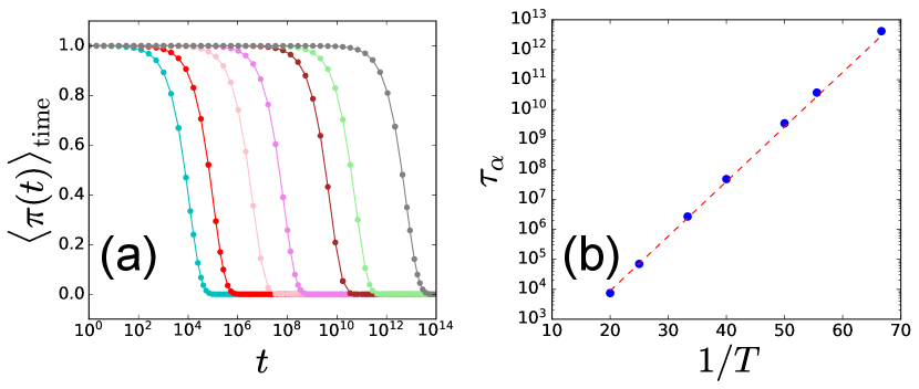
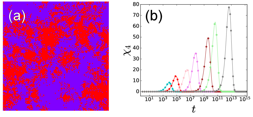
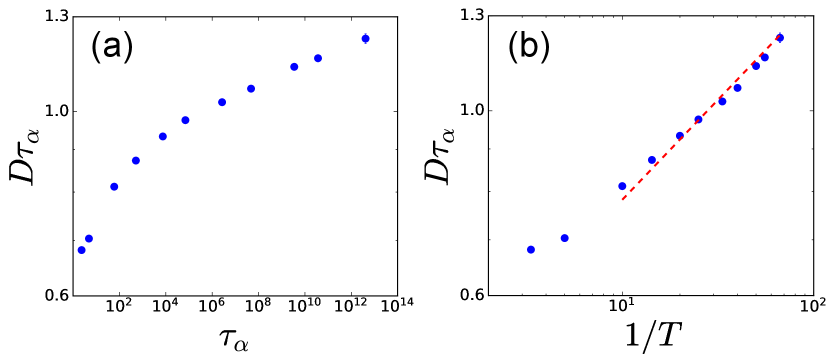
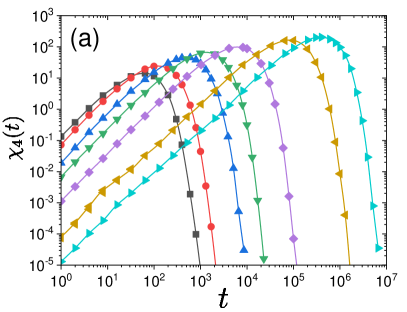
We first perform finite temperature simulations and characterize dynamical properties. To this end, we consider the persistence two-point time correlation function, , which has been used widely in the context of kinetically constrained models Ritort and Sollich (2003). The observable is defined by , where if the site did not exhibit a plastic event until time and remained immobile, and for mobile sites that relaxed at least once. The notation denotes the time average at the stationary state at temperature reached after a long enough equilibration time. We have verified that the model does show dynamical slowing down by measuring at different temperatures, as shown in Fig. 1(a). In Fig. 1(b), we find that the associated relaxation time defined by increases in a Arrhenius way. Figure 2(a) represents a snapshot of local persistence for , demonstrating spatially heterogeneous dynamics. To quantify the magnitude of dynamical heterogeneity, we compute the four-point correlations function Donati et al. (2002), , defined by
| (1) |
is proportional to the size of the dynamically correlated region (see Appendix B for details), which is the central observable characterizing dynamical heterogeneity approaching the glass transition Berthier et al. (2011), as it has been estimated in real experiments Berthier et al. (2005); Dalle-Ferrier et al. (2007); Capaccioli et al. (2008); Dauchot et al. (2022) as well as molecular simulations Donati et al. (2002); Karmakar et al. (2009); Coslovich et al. (2018).
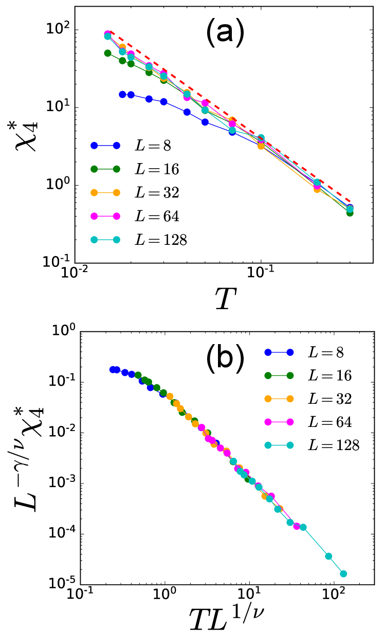
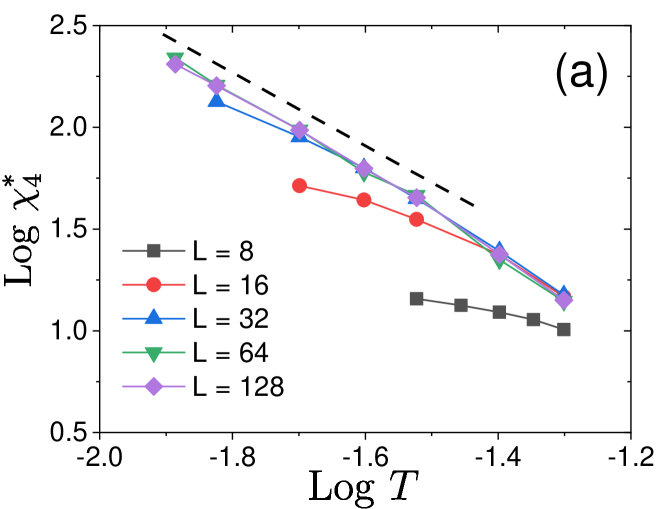
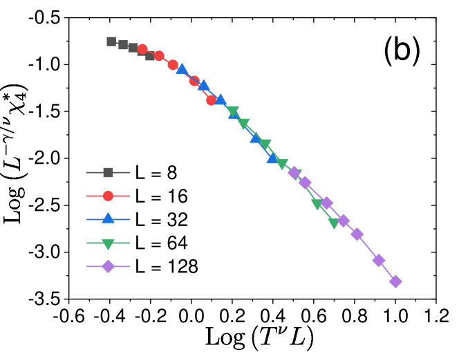
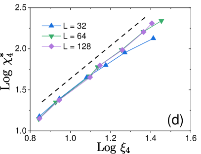
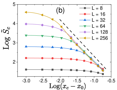
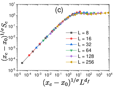
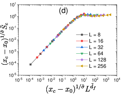
Figure 2(b) shows the time and temperature evolution of . It takes a peak near the relaxation timescale , and the peak grows with decreasing temperature, which is the hallmark of dynamical heterogeneity in glassy dynamics. We have then plotted the peak value of , denoted , versus temperature for several system sizes in Fig. 3(a). The system size dependence, akin to molecular simulations Karmakar et al. (2009); Chakrabarty et al. (2017), allowed us to perform finite size scaling. We find that for increasing the system size , follows a scaling form, with a critical point at and the associated exponent . We obtain a scaling collapse for in Fig 3(b) (see also molecular simulation studies Karmakar et al. (2009); Chakrabarty et al. (2017)), indicating that the dynamics is governed by a diverging correlation length toward , i.e., with an exponent . The corresponding data for the scalar model are presented in Appendix B. Besides, we obtained a consistent result in terms of by directly measuring the dynamical correlation lengthscale based on the four-point structure factor Lačević et al. (2003). The observed critical exponents and predictions (see below) are summarized in Table 1. The main goal of this paper is to provide a scaling theory for these critical behavior, connecting the dynamics at finite temperature to a zero-temperature critical point.
| Scalar model | Tensorial model | Pred. | Pred. MF | |
|---|---|---|---|---|
IV Critical Point and Extremal Dynamics at
We now consider dynamics at vanishing temperature, , and show that it is related to a critical point. At the site with the smallest energy barrier , the weakest site, always yields first 222We are considering either finite systems or the thermodynamic limit taken after the zero-temperature limit., where is the corresponding stress required to destabilise the site. Therefore, one can simulate dynamics at by relaxing always the weakest site, instead of relaxing a random site weighted by the relaxation rate . This algorithm allows us to access dynamical information even at vanishing temperature (see details in Appendix C). It is an example of extremal dynamics, which is well-studied in the context of self-organized-criticality Paczuski et al. (1996) and some disordered materials under quasi-static driving Baret et al. (2002); Purrello et al. (2017), including annealed glasses Kumar et al. (2022).
In the thermodynamic limit, , the extremal dynamics leads to an absorbing condition for , where is a critical energy barrier as found (for ) in Ref. Ozawa and Biroli (2023). As a result, the distribution of local (activation) energy barriers vanishes for (see the sketch in Fig. 9(a)). This implies that for , where is the distribution of . Thus only a sub-extensive number of sites are found for at a finite . In this paper, we use and interchangeably since they carry essentially the same information.
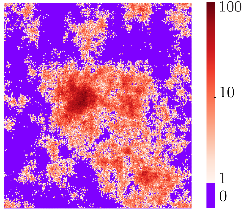
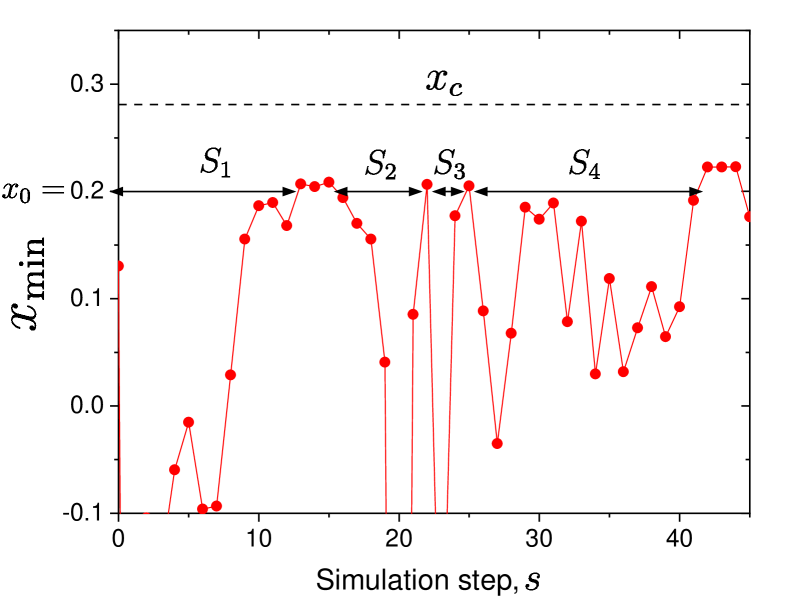
The extremal dynamics consists of a succession of avalanches. In fact, relaxation at a site can change local energy barriers at different sites by elastic interactions. As long as those are below the corresponding sites belong to the same avalanche Paczuski et al. (1996). This is a vivid realization of the phenomenon of dynamic facilitation. To characterize the avalanches, we follow the method introduced in the study of extremal dynamics Paczuski et al. (1996); Purrello et al. (2017). For a finite , we fix a chosen threshold stability value , and define -avalanches as the sequences of events for which (see Fig. 16 in Appendix C). Two useful characterizations of avalanche size are the total number of relaxation events in a given sequence (event-based avalanche size), and the total number of sites that relaxed at least once during an avalanche (site-based avalanche size). By construction, and . We show snapshots having and the corresponding in Fig. 4. The two can be (and, as we shall show, are) different as a site can relax multiple times within the same avalanche. Thus, the event-based avalanche size will allows us to quantify the accumulation of relaxation events in the mobile region (as emphasized in a recent molecular simulation study Scalliet et al. (2022)), whereas the site-based avalanche size will be associated to the spatial extent of dynamically correlated regions (as it contains the essentially same information as the persistence map in Fig. 2(a) and hence ). Sizes of avalanches, and , depend on the threshold . They grow with increasing and diverge at .
By systematically exploring different values of one can determine the critical point . In fact, one expects that the avalanche distribution during the extremal dynamics follows a power-law with a scaling form Paczuski et al. (1996); Purrello et al. (2017); Han et al. (2018):
| (2) |
where is a scaling function and is a cutoff size which takes the form:
| (3) |
where and are critical exponents and for and for . Thus, when , whereas when . The same expressions are expected to hold for the site-based avalanche size , defining exponents , , and . To estimate we use the fact that for the ratio is proportional to the cutoff value , where . As we are interested in scaling of with system size, the numerical constant is irrelevant and we define . The same expression is used mutatis mutandis for the site-based avalanche size, . More details about avalanche statistics can be found in Appendix C.
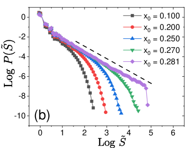
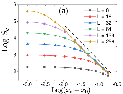
We determine and the exponents , , and by measuring and for different values of threshold and system size and collapsing them using the scaling form in Eq. (3) for both and , as shown in Figs. 5 (a, b). We obtain . The values of the critical exponents are presented in Table 2. Figures 5 (c, d) display and as a function of , for various system size . They indeed show that and grow with and saturate due to finite size effects.
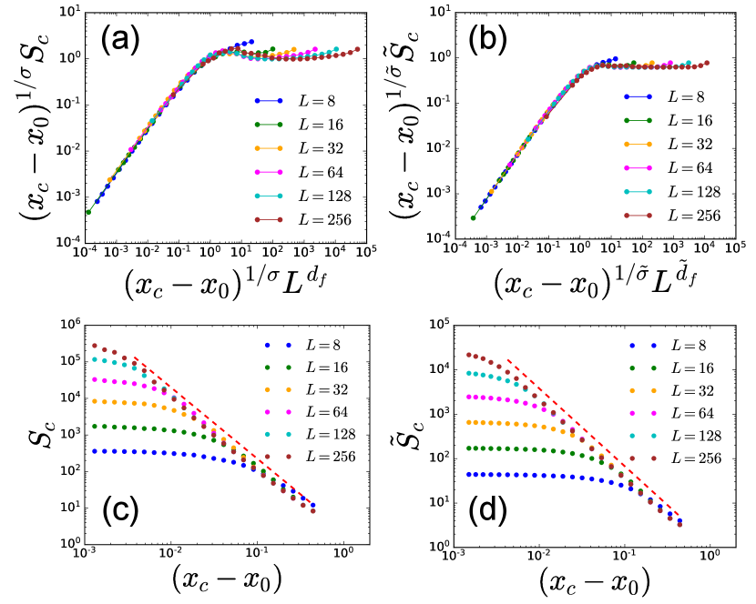
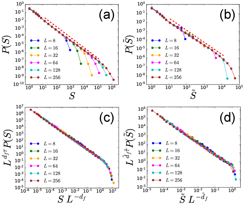
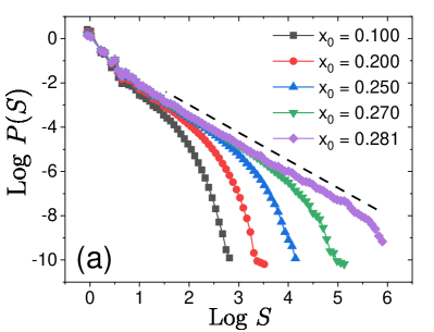
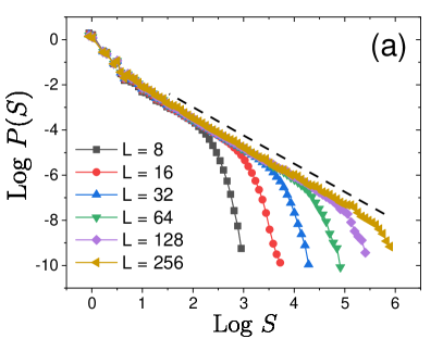
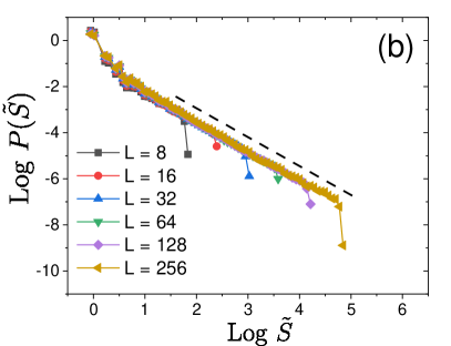
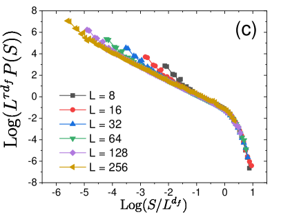
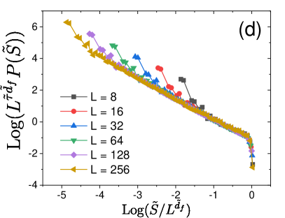
Once is determined, we can study the statistics of the system-spanning avalanches relevant to the thermodynamic limit. Thus, we fix and measure the distribution and of the avalanche sizes, see Figs 6 (a,b). We find that avalanche sizes are power-law distributed with eventual cut-off, consistent with the general assumption in Eq. (2). The scaling form in Eq. (2) collapses the data using and the previously obtained values of and , see Figs 6 (c,d). From the data collapse we determine values of avalanche exponents and (see Table 2). The successful collapse of the data confirms the validity of the scaling ansatz as well as the value of critical exponents.
The above analysis reveals that the extremal dynamics of our model of glass forming-liquid displays, scale-free, avalanche-type dynamics akin to the ones of other disordered systems under external loading Sethna et al. (2001); Rosso et al. (2022).
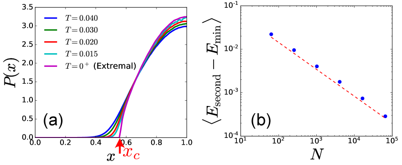
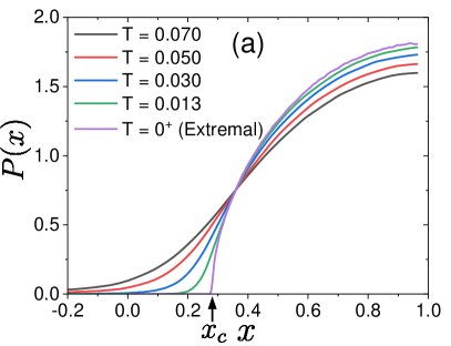
Coming back to the distribution of energy barriers and the corresponding distribution , one would expect that it continuously vanishes at as , defining an exponent Popović et al. (2021). This behavior also occurs near the yielding transition of amorphous solids under shearing (with ) Lin et al. (2014b), where it affects the scaling of flow properties Lin et al. (2014a) and plasticity Karmakar et al. (2010), and more generally in glassy systems with long-range interactions Müller and Wyart (2015). The underlying reason is that at each step of the extremal dynamics, each site receives a stress kick, such that of a site follows a random process, with an effective absorbing condition at . If this random process was a Brownian motion, then one would obtain . Yet the kicks are much more broadly distributed, and in higher dimensions, this random process is akin to a Levy flight Lemaître and Caroli (2007), which can be shown to imply Lin and Wyart (2016). In Fig. 7(a), we plot for the extremal dynamics, measured from configurations just before (or after) each avalanche defined as , together with obtained from finite temperature simulations studied in Sec. III. At higher , shows a broader distribution with a smooth decay. As is decreased, converges to the one obtained by the extremal dynamics at , whose shape is consistent with .
The following two features of connect the extremal and finite temperature dynamics. First, the point or the corresponding energy scale controls the effective energy barrier associated to . Indeed, at small temperature the dynamics proceeds by relaxing the sites with smallest barriers, i.e., sites having barriers close to Ozawa and Biroli (2023); Popović et al. (2021). This is in agreement with the relaxation time observed in Fig. 1(b), which scales as .
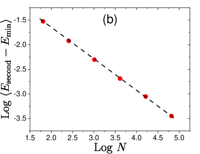
Second, more importantly for what follows, in a finite system of size , the typical scale of and the second lowest , denoted as , is expected to follow a power law, . As we shall show, this plays a key role in the characterization of thermal avalanches. Since the energy difference between the lowest and second lowest activation energies is given by , we conclude
| (4) |
Thus the exponent characterizes an important feature of the energy barrier relevant for low temperature dynamics. We numerically confirmed this scaling in Fig. 7(b), and the obtained value of is reported in Table 2. Extreme value statistics argument would suggest Lin et al. (2014a) (although near the yielding point deviations from this relation have been reported in finite dimension Ferrero and Jagla (2021), and explained in Korchinski et al. (2021)). Within the mean-field theory Lin and Wyart (2016), one finds , a value close to what we observe in Fig. 7(b).
The results presented in this section show that the extremal dynamics of the tensorial elastoplastic model of super-cooled liquids is governed by system-spanning avalanches. We have fully characterized the associated zero temperature critical point by obtaining all relevant exponents, summarized in Table 2. We also obtained qualitatively and quantitatively (e.g., critical exponents) similar results in the scalar model, which are presented in Appendix C. Remarkably, we find that the scalar and tensorial models display very close values of the critical exponents and likely correspond to the same universality class.
| Scalar model | Tensorial model |
|---|---|
V Scaling theoretical arguments
In the following, we develop a scaling theory that connects dynamical heterogeneities observed in finite temperature simulations (Sec. III) and the zero-temperature critical point, and associated avalanches, of the extremal dynamics (Sec. IV). We will also discuss other important physical consequences, such as the time evolution of avalanche sizes and the Stokes-Einstein violation.
V.1 Length scale of dynamical heterogeneity
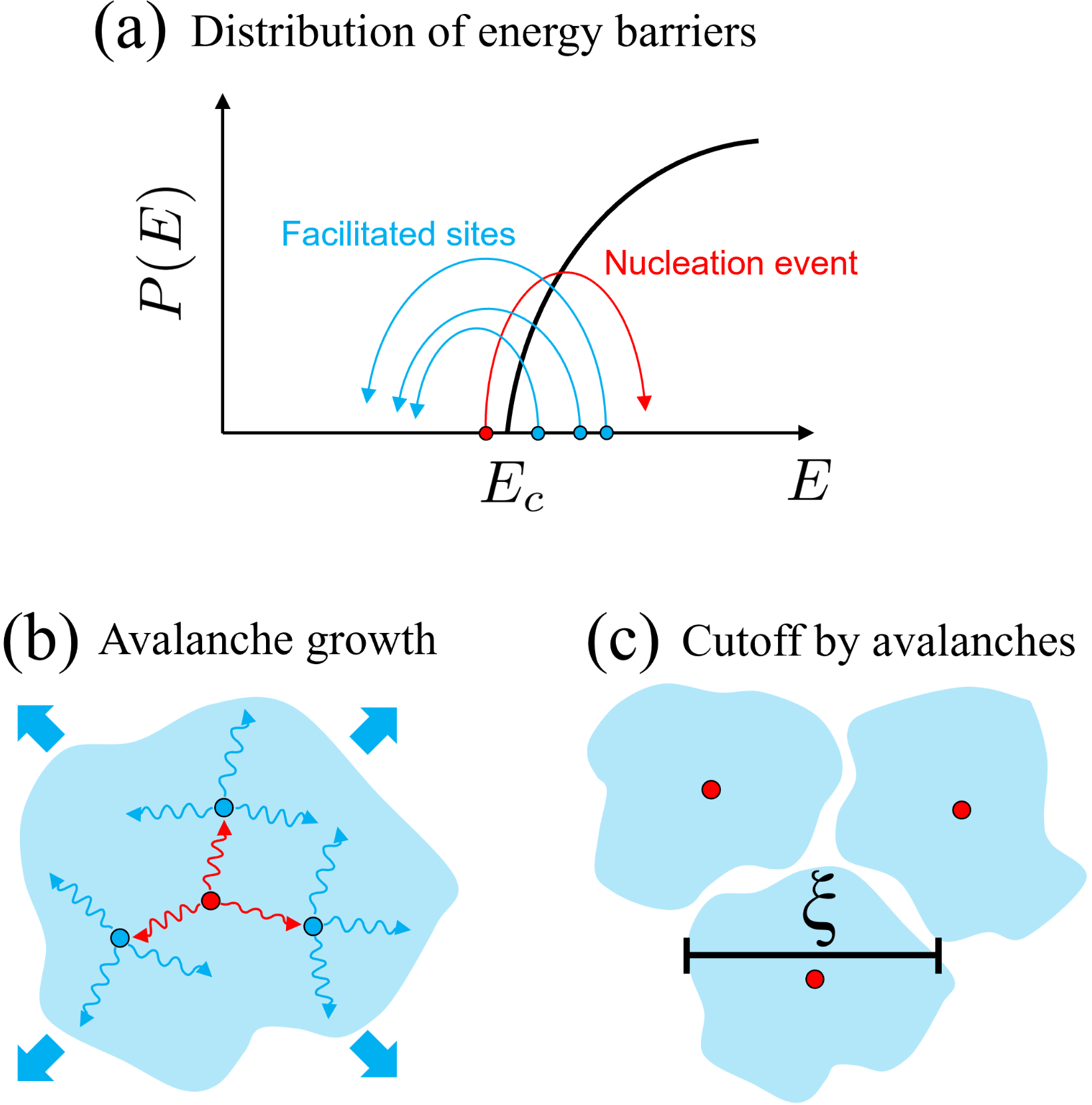
We consider the effect of finite temperature on the extremal dynamics. As we will discuss below, the breakdown of the condition for the extremal dynamics naturally leads to the lengthscale of dynamical heterogeneity at finite . The proposed picture is schematically depicted in Fig. 9.
At finite but low , the dynamics is expected to be extremal on large but finite lengthscales. To understand the underlying mechanism, let us consider a finite size system. For a fixed system size, if is small enough, the site with the lowest activation energy typically relaxes first like for (the probability to relax the site with the second lowest energy is negligible). This relaxation corresponds to a slow ”nucleation” event when that occurs on a timescale , as schematically shown in Fig. 9(a). The nucleation event lowers energy barriers of some other sites of the system, which we call ”facilitated” sites, due to elastic interactions, and causing a sequence of faster events when , as shown in Fig. 9(b). This cascade process forms an avalanche, which eventually stops. A new avalanche starts again once another nucleation event occurs. The dynamics is thus intermittent with the power-law avalanches discussed in Sec. IV. Clearly, there is a typical size above which this picture breaks down. Indeed, the above description holds when the thermal energy is much smaller than the typical energy difference between the lowest and second lowest activation energies, , otherwise sites with higher energy barriers (such as ) might relax and dynamics cease to be extremal. According to Eq. (4), depends on the system size . Thus, the condition for the extremal dynamics which interplays and is given by , i.e., .
In consequence, when the system size is too large at fixed , the above description cannot hold. In this case, in particular in the thermodynamic limit, multiple nucleation events followed by avalanches will take place (independently) in parallel in the system, as sketched in Fig. 9(c). The cut-off length scale encompassing a single avalanche is not limited by system size but by other avalanches in the system, which can be estimated assuming that the locations of these avalanches are independent. Such an approximation will be accurate if structural spatial correlations are not prepunderant in this system, as discussed below. Assuming finite size scaling, must then corresponds to the largest system size for which extremal dynamics at finite holds, i.e., . This provides the link between finite size zero-temperature avalanches and thermal ones. Moreover, it also directly predicts that the size of dynamically correlated regions characterized by , which is given by the cross-over size above which the condition for the extremal dynamics breaks down: leading to . To conclude, we derive two scaling relations for thermal avalanches:
| (5) | |||||
| (6) |
These scaling relations connect dynamical heterogeneities at finite (characterized by and ) and the distribution of local energy barriers at (characterized by ) together with the morphology of avalanches during the extremal dynamics (by ). We thus predict and by using and measured in the extremal dynamics in Sec. IV. These predictions are in good agreement with finite temperature simulations in Sec. III, as summarized in Table 1. We also find that the mean-field predictions using and lead to similar values.
This argument is expected to break down if large spatial correlations characterize the structure of the system, causing the locations where avalanches start to be correlated. Indeed, as is always the case in disordered materials at zero temperature, any critical threshold such as or must display finite-size fluctuations . These fluctuations are described by some exponent , such that in a system of finite size , one has . The value of is affected by spatial correlations. In general one must have , since the fluctuations of or must be at least as large as the typical distance between most unstable sites in a quiescent system : indeed, cannot be more precisely defined than this difference. We expect our argument above to hold when , corresponding to . can be related to previously introduced exponents, and , as follows. If a finite system displays a system spanning avalanche and entirely rearranges, then the change of , or equivalently that of , must be of order . According to Eq. (3), an avalanche of size is associated with a characteristic change of the critical threshold (when in ), implying that . Since and , we obtain . Using numerical values for and , this expression leads to and , respectively, for the scalar and tensorial models. We thus have in the present system , supporting our assumption of independent avalanches. Note however that such an equality does not need to hold in general, especially in large .
V.2 Time evolution of thermal avalanches
We now focus on the time evolution of the size of thermal avalanches, based on the scaling results for the extremal dynamics. In Sec. IV, we introduced -avalanches to more generally probe the critical behavior at . This turns out to be useful also to work out the relationship between time and length scales for thermal avalanches. In fact, is associated to a typical energy scale . Hence, it carries information both about the typical time-scale and the avalanche (cut-off) size .
According to the scaling argument discussed before, even at a finite temperature , the extremal dynamics can be applied to a finite system, in particular, smaller than . The cutoff size of -avalanches, , follows , see Eq. (3) and Fig. 5(b). During an extremal dynamics, the duration of an avalanche will be dominated by the relaxation of the most stable site it involves, of characteristic timescale . We thus obtain a relation connecting the duration of avalanches, (measured in the unit of the relaxation time ), with the cutoff size as . Therefore, avalanches in such a finite system and over a finite time interval (smaller than the relaxation time scale ) are intermittent. Namely, the system is quiescent most of the time, yet when it is not, its avalanche size is power-law distributed with a cutoff size , which is given by
| (7) |
Thus, we find that the size of avalanches grows very slowly – only logarithmically – with time.
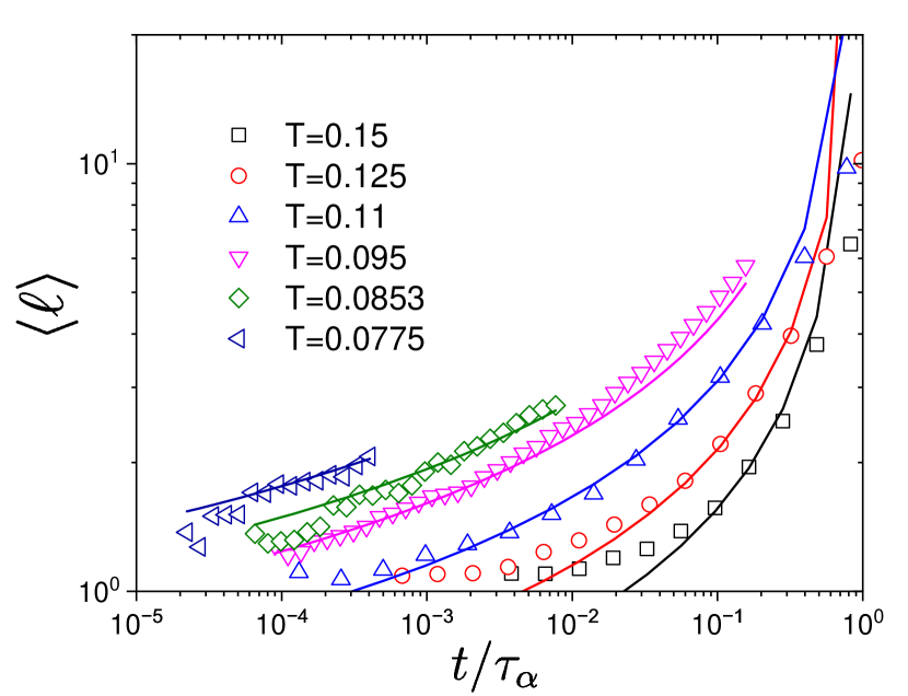
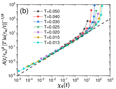
The above prediction can be tested experimentally or in molecular dynamics simulations Candelier et al. (2010); Scalliet et al. (2022). In Ref. Scalliet et al. (2022), the time evolution of a chord length characterizing the linear size of mobile domains has been measured. Since we expect , our prediction for is given by
| (8) |
where is a function with a finite limiting value as . In Fig. 8, we compare the molecular simulation data for a two-dimensional polydisperse mixture Scalliet et al. (2022) and our prediction. The prediction is very good, in particular, at lower temperatures where the elastoplastic description is supposed to work well.
In Appendix B, we also connect and explicitly. This allows us to predict the time evolution of for times – a prediction that agrees with the numerics.
V.3 Decoupling between diffusion and relaxation
We now show that the scaling theory developed above directly implies decoupling between diffusion and relaxation as found in super-cooled liquids, the so-called Stokes-Einstein violation Tarjus and Kivelson (1995); Ediger (2000); Sengupta et al. (2013); Charbonneau et al. (2014); Kawasaki and Kim (2017).
One of the remarkable aspects found in the numerical simulations in Sec. IV is that sites relax multiple times within the same avalanche. In terms of a dynamical trajectory, a site waits a long time (remains immobile) before relaxing, but once it relaxes, it redoes multiple times within a short period of time. This is characterized by a difference between the so-called persistence time and exchange time Jung et al. (2004); Berthier et al. (2004); Hedges et al. (2007) (or the caging time in molecular simulations Ciamarra et al. (2016); Pastore et al. (2021)), which has been argued to be the key ingredient of decoupling between diffusion and relaxation in super-cooled liquids Jung et al. (2004); Berthier et al. (2004); Hedges et al. (2007); Chaudhuri et al. (2007); Pastore et al. (2021).
In our case, this effect originates from the difference between the event-based and site-based avalanche sizes characterized by . To connect it to the zero temperature critical point, let us focus on the formation of a thermal avalanche whose time-scale is the order of and liner size is . During the formation, a single site relaxes order of times. Assuming that each relaxation gives a random displacement to particles in the neighborhood of this site, their diffusion constant must be proportional to the rate for the relaxation event, , leading to a Stoke-Einstein breakdown of order that diverges at vanishing temperature with . Conventionally, the Stokes-Einstein violation is considered a consequence of spatially heterogeneous dynamics Ediger (2000). We directly connect the former and the length scale of dynamical heterogeneity . On top of that, our scaling theory emphasizes accumulations of multiple events inside a mobile region as the microscopic mechanism leading to the Stokes-Einstein violation.
Note that our scaling argument does not predict a fractional Stokes-Einstein violation in which , or , but instead where . The former is the fit that is usually conjectured from experimental data Swallen et al. (2003); Mallamace et al. (2010) with . However, given the small value of the latter fit is also a viable option 333In fact, in some kinetically constrained models Garrahan et al. (2011), the fractional Stokes-Einstein violation (with a similar value of with experiments) was conjectured based on numerical data and physical arguments. Recent rigorous results Blondel and Toninelli (2014) showed that this is not what happens, but there is likely a violation as the one we find. This suggests that the logarithmic Stokes-Einstein violation can be easily misinterpreted as a fractional one with a small exponent ..
We have numerically tested our prediction for the Stokes-Einstein violation in Fig. 10, showing the product in the tensorial model. In this plot, is estimated numerically using tracer particles that jump randomly by one lattice spacing each time relaxation occurs in their current site, similarly to what was originally done for kinetic constrained models Jung et al. (2004); Berthier et al. (2004) (see Appendix B for details). increases with decreasing , following the scaling prediction with measured independently in Secs. III and IV. The observed amount of the violation we find is not large and hence more representative of strong glass-forming liquids than fragile ones since it has been reported that the magnitude of the violation and fragility are correlated Ediger (2000); Ozawa et al. (2016). We will come back to this point in Sec. VI.
VI Conclusion and discussion
We provided a theoretical description of dynamical heterogeneities in super-cooled liquids based on the assumption that local rearrangements are elastically coupled. The elasto-plastic models we studied offer a quantitative solution for how dynamical correlations can emerge even in cases in which local barriers control the dynamics Glarum (1960); Dyre (2006); Lerbinger et al. (2022); Hasyim and Mandadapu (2021); Ciamarra et al. (2023). Our main result is the theoretical explanation of dynamical correlations in terms of a zero-temperature critical point with the associated scaling relations. This leads to quantitative predictions on the power-law statistics of thermal avalanches testable in more realistic systems. Our study suggests that dynamical heterogeneities in super-cooled liquids should be investigated in terms of the temperature to seek power-law relations, rather than in terms of the relaxation time scale.
One important aspect of the models we studied is that they encode in a very simple and natural way the coupling of local relaxation and elastic interaction. Their simplicity, combined with the richness of the dynamical behavior – in particular, the emergence of facilitation and dynamical correlations – is a remarkable aspect, as it shows which salient facts one can obtain with minimal physical ingredients. Kinetically constrained models have instead abstract kinetic rules and show a large variety of behaviors depending on the kinetic constraints Ritort and Sollich (2003). Although local excitations identified in the dynamic facilitation scenario Isobe et al. (2016); Keys et al. (2011) would have connections with local activations in our framework, the physical interpretation of kinetic rules in kinetic constrained models is still an open and crucial challenge. Along this line of thought, it would be interesting to devise a kinetic constraint rule effectively incorporating elastoplasticity. Nevertheless, various concepts and theoretical tools developed in the study of kinetically constrained models provide important guidelines and, in fact, played an essential role for our analysis of thermal elasto-plastic models. It has been demonstrated in the dynamic facilitation theory that a critical point in an extended non-equilibrium phase diagram influences glassy dynamics Elmatad et al. (2010); Turci et al. (2017). It would also be interesting to study whether such a critical point exists in elastoplastic models.
Quantitatively, the magnitude of dynamical heterogeneities we simulated is comparable to most super-cooled liquids (as the estimated increases by about two decades as the glass transition is reached Dalle-Ferrier et al. (2007); Dauchot et al. (2022)), whereas the magnitude of the Stoke-Einstein breakdown is comparable to that of rather strong glass-forming liquids Ediger (2000). According to our scaling argument, such a breakdown will increase if the system shows more intensive accumulations of multiple relaxations characterized by larger . This effect could be achieved by imposing that some of the model parameters (such as the local values of the yield stress, or how sites are coupled to the elastic field) are randomly distributed Agoritsas et al. (2015), instead of being single-valued as assumed here for simplicity. These effects are expected in glass-forming liquids due to the presence of structural heterogeneity of local orders Tanaka et al. (2010); Royall and Williams (2015); Tanaka et al. (2019); Paret et al. (2020). Such generalization would allow us to study the structure-dynamics relationship Widmer-Cooper et al. (2004, 2008); Hocky et al. (2014) in elastoplastic models. Further improvements may be achieved by adding fluctuations and non-linearities to the propagator, which are present at short-range Lemaître et al. (2021); Lerner et al. (2014). An interesting line of research to develop quantitative models is a mapping from a molecular simulation to an elastoplastic model Liu et al. (2021); Castellanos et al. (2021, 2022) or the one pursued in Refs. Tah et al. (2022); Xiao et al. (2023), which uses machine learning methods and the so-called softness field to obtain quantitative effective models.
Our results also underline important themes to study in the future, including the nature of local rearrangements in glass-forming liquids, and their connection to fragility Ediger et al. (1996). Concerning the latter, the current elastoplastic models correspond to strong glass-formers with Arrhenius behavior, with activation energy given by the magnitude of the gap entering the distribution of local barriers Popović et al. (2021); Ozawa and Biroli (2023). This point results from the simplifying assumption that the energy scale of local rearrangements does not vary with temperature. In an improved (still simplified) model where all elastic energies follow the high-frequency elastic modulus of the material, the activation energy will be proportional to , a correlation known to exist in some glass-forming liquids Dyre (2006); Hecksher and Dyre (2015). More recent works relate this energy scale of local rearrangements to local (instead of global) elasticity Kapteijns et al. (2021), plasticity Lerbinger et al. (2022), or alternatively to the varying geometry of elementary rearrangements under cooling Ji et al. (2022). Thus, it is worthwhile to reveal the relationship between the activation energy barriers in liquids and low-energy excitations in glasses Scalliet et al. (2019); Mizuno et al. (2020); Richard et al. (2023). Local energy barriers would also be related to locally-favored structures in microscopic perspectives Coslovich and Pastore (2007); Royall and Williams (2015). More progress along those lines will be instrumental to understand what controls fragility in glass-forming liquids.
Note that although we mainly focused our attention on the theoretical scenario based on local barriers driving the dynamics Kapteijns et al. (2021); Lerbinger et al. (2022); Ciamarra et al. (2023) together with facilitation and avalanches, the physical phenomena discussed in this work are more general. For example, they can also apply to cases in which cooperative rearrangements take place. In these perspectives, in particular within Random First Order Transition theory, the local relaxation event would correspond to a cooperative rearrangement Scalliet et al. (2022); Biroli and Bouchaud (2022). Obviously, our current elastoplastic models do not take into account growing cooperativity as a static correlation, and they have a singularity only at in contrast to RFOT with a finite temperature singularity at . One could incorporate a growing static correlation in the models by increasing the number of sites involving a thermal activation process. It would be interesting to work out precise predictions in this case.
Finally, we expect our scaling theory which connects spatial correlations at finite temperature to extremal dynamics at zero temperature, to be relevant for a broader class of problems beyond the context of the glass transition studied here. Phenomena in which the implications of these arguments could be studied include the creep flow of disordered materials Castellanos and Zaiser (2018); Bauer et al. (2006); Caton and Baravian (2008); Divoux et al. (2011); Siebenbürger et al. (2012); Grenard et al. (2014); Leocmach et al. (2014) or that of pinned elastic interfaces Bustingorry et al. (2007); Purrello et al. (2017); Kolton et al. (2005) below the threshold force where they spontaneously flow.
Acknowledgement
We thank the Simons collaboration for discussions, in particular J. Baron, L. Berthier, C. Brito, C. Gavazzoni, E. Lerner, C. Liu, D. R. Reichman, and C. Scalliet. We thank S. Patinet for insightful discussions. We appreciate C. Scalliet for sharing the data in Ref. Scalliet et al. (2022). GB thanks J.P. Bouchaud for discussions, in particular on the Bak-Sneppen model and models of dynamic facilitation. MW thanks A. Rosso and M. Muller for discussions on avalanche-type response over the years, and T. de Geus, W. Ji and M. Pica Ciamarra for discussions. MW acknowledges support from the Simons Foundation Grant (No. 454953 Matthieu Wyart) and from the SNSF under Grant No. 200021-165509. GB acknowledges support from the Simons Foundation Grant (No. 454935 Giulio Biroli).
Appendix A Thermal elastoplastic models
A.1 Scalar model
We study a scalar elastoplastic model Ozawa and Biroli (2023) in a two-dimensional lattice whose linear box length is using the lattice constant as the unit of length. For each site, we assign local shear stress (scalar variable) at a position .
The dynamical rule for the simulation model is akin to Monte-Carlo dynamics Berthier and Kob (2007). We pick a site, say , up randomly among sites. If is greater (or lower) than or equal to a threshold (or ), namely, , this site shows a plastic event: , where is the local stress drop. We use an uniform threshold, . Instead, if , with probability , where is a local energy barrier and is the temperature, this site shows a plastic event: . This corresponds to a plastic rearragement induced by a local thermal activation. We employ with Maloney and Lacks (2006). By introducing the local stress distance to threshold, , we can rewrite . This specific form of the local energy barrier is suggested by molecular simulation studies Fan et al. (2014); Lerbinger et al. (2022) and previous elastoplastic models under shear Popović et al. (2021); Ferrero et al. (2021). The stress drop associated with a plastic event is a stochastic variable. In this paper, we use , where is the sign function and is a random number drawn by an exponential distribution, . is the mean value and we set . This exponential distribution would be realistic according to molecular simulations in Ref. Barbot et al. (2018).
A local plastic event at site influences all other sites () as
| (9) |
where and is a random orientation of the Eshelby kernel . Numerical implementation of is described in Ref. Ozawa and Biroli (2023).
Similar to the Monte-Carlo dynamics, we repeat the above attempt times, which corresponds to unit time.
For the initial condition, we draw the local stress randomly while keeping the force balance, i.e., the sum of stresses along each row and column of lattice sites is strictly zero Popović et al. (2018); Pollard and Fielding (2022). To study dynamical properties at the steady-state, we monitor the waiting time dependence of observables, and we report them only at the steady-state, discarding the initial transient part.
A.2 Tensorial model
We have implemented a two-dimensional elastoplastic model in which we account for the tensorial nature of the shear stress tensor. In this tensorial version of the elastoplastic model, the state of each site is described by its local shear stress tensor . Note that symbols and are also used as critical exponents in the main text, not to be confused with local shear stress defined here. The shear stress tensor is traceless and symmetric and hence in two dimensions it is defined by two independent components: and .
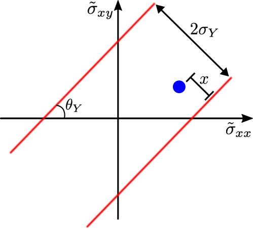
The local yield stress is defined by a surface in the shear stress space, with the region inside and outside the surface corresponding to mechanically stable (elastic, immobile) and unstable (plastic, mobile) states, respectively. The minimum amount of shear stress required to make a site unstable is the distance to the yield surface, and we denote its magnitude by , as schematically shown in Fig 11. We choose the local yield surface to consist of two parallel lines at an angle with respect to the axis in shear stress space, centered at zero shear stress and separated by (see Fig 11). The local yield surface is assigned for each site . We initiate with a uniformly distributed random number in .
When a site becomes unstable it undergoes a plastic event over a timescale : and , where the amount of stress drops and are given by
| (10) | ||||
| (11) |
respectively. is the sign function and is a random number drawn from an exponential distribution with . The duration of a plastic event is accounted for by triggering the relaxation with a probability per unit time whenever the site is unstable. In an athermal system sites can only relax by first becoming unstable. At finite temperature stable sites undergo relaxation at the rate , where is the local energy barrier Popović et al. (2021). After each plastic event, we redraw the angle of the yield surface from a uniform random distribution.
.
Note that to simulate such a dynamics at low temperatures we implement a Gillespie type of algorithm Popović et al. (2021), which operates as follows. Consider an event occurring at some time . Following it, a relaxation time for each site is chosen with an exponential distribution of mean . The next event corresponds to the smallest , leading to a plastic event on the corresponding site, which occurs at a time . At that point, stresses are computed once again, the variables are sampled from their new distributions. this algorithm is then repeated iteratively.
To maintain the force balance, a plastic event at site redistributes the shear stress field in the other sites following the force dipole propagator. In Fourier space the elements of elastic kernel are given by,
| (12) | ||||
| (13) | ||||
| (14) |
where is the Fourier vector. For a discrete system with periodic boundary conditions, we introduce a correction term to the Fourier modes, given by , and where with .
Appendix B Characterizations of dynamical heterogeneities for finite temperature simulations
B.1 Four-point correlation function
We explain how to analyze correlation functions for finite temperature simulations. We first consider the persistence two-point time correlation function, , which is defined by , where (immobile) if the site did not show a plastic event until time from , and (mobile) otherwise. denotes the time average at the stationary state. for the scalar and tensorial models are presented in Fig. 1 of Ref. Ozawa and Biroli (2023) and Fig. 1(a) in the main text, respectively. We then measure a four-point correlations function, , defined by
| (15) |
for the scalar and tensorial models are presented in Fig. 3 of Ref. Ozawa and Biroli (2023) and Fig. 2(b) in the main text, respectively. quantifies the size of the dynamically correlated region, because one can rewrite it as
| (16) | |||||
| (17) |
where . For example, . Therefore, is proportional to the average number of sites correlated dynamically. Therefore, its peak value, , contains essentially the same information as , in particular, at .
Figure 12(a) shows versus for several system sizes for the scalar model. One can see a scaling regime, at lower and larger . A scaling collapse is obtained in Fig. 12(b), which determines another critical exponent associated with a lengthscale of dynamical heterogeneity. The obtained values for the critical exponents are reported in Table 2.
B.2 Dynamical correlation lengthscale
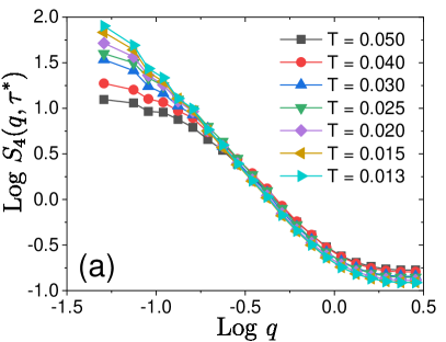
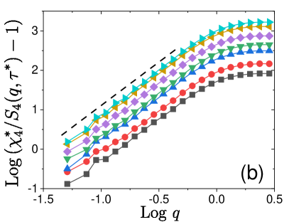
We consider extracting a correlation length directly instead of performing finite-size scaling. To this end, we measure the spatial dependence of the four-point structure factor, Lačević et al. (2003), defined by
| (18) |
where . In Fig. 13(a), we show for the scalar model at when takes the peak value, . We find that is close to , and thus encodes heterogeneity associated with structural relaxation. We note that at the long wave-length limit, converges to , namely, . We then assume the Ornstein-Zernike form at lower ,
| (19) |
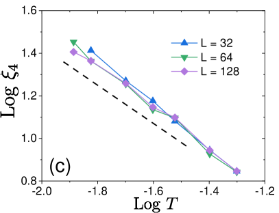
where is the dynamical correlation length extracted and is an exponet. As shown in Fig. 13(b), we find this scaling with . From this plot, we extract and present its temperature dependence in Fig. 13(c). This analysis can be done only for larger systems, , , and , since the scaling regime cannot be reached in smaller systems within our simulations. We find with , which is consistent with the one estimated from the finite size scaling in Fig. 12. Moreover, the versus plot Flenner et al. (2014); Kim and Saito (2013) in Fig. 13(d) provides us with the fractal dimensions, , which is also consistent with the one measured in the extremal dynamics in Fig. 18.
B.3 Prediction for the four-point correlation function
We connect the cutoff size for the site-based avalanche size, , in a given time interval , and the time evolution of the four-point correlation function, .
We first compute the site-based avalanche size by , where if the site did not exhibit a plastic event until time , and for mobile sites that relaxed at least once. Thus, can be written by . The first and second moments of measured by the time average are given by
respectively. Consider a correlation volume of linear extension . On this length scale, crosses-over toward its value for an infinite system. It is also the largest length for which extremal dynamics applies, implying that is distributed in a power-law fashion. Thus, can be estimated by , as given by
| (20) |
In general, one can expect that follows the (stretched) exponential decay, , where is an exponent. Typically, for equilibrium supercooled liquids. Our elastoplastic models show nearly exponential relaxation with . We now consider the early time stage, where can be approximated by . Under such a circumstance, Eq. (20) and defined in Eq. (16) suggest that . Together with Eq. (7) in the main text, we predict the time evolution of as
| (21) |
where is a constant which does not depend on and .
Figure 14(a) shows a Log-Log plot for measured at finite temperature simulations for the scalar model. The initial growth can be fitted effectively by a power-law, Biroli et al. (2022); Flenner and Szamel (2016), with . Instead, our argument in Eq. (21) predicts a linear growth with a logarithmic correction. In Fig. 14(b), we show a parametric plot to numerically test Eq. (21) with , , and (see Table 2). We find that the simulated for different temperatures follows our prediction at early times. Deviations from the prediction can be observed on very short timescales. This is presumably due to the fact that on such time scales, the corresponding energy scale is too small compared with , which violates the assumption underlying the asymptotic argument of Sec. V.
B.4 Tracer particles
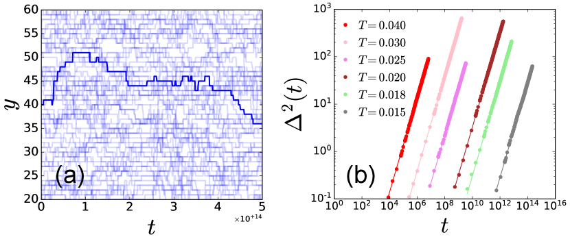
We monitor the diffusion of tracer particles Jung et al. (2004); Berthier et al. (2004) due to the local relaxations. We consider one tracer particle in each site of the elastoplastic model; each tracer particle moves randomly to one of the four nearest neighbors (in ) after a plastic event in that site. The trajectory of the -th tracer particle is specified by . Typical trajectories of the tracer particles are shown in Fig. 15(a) as a function of time. In a time scale comparable to , the tracer travels over multiple sites in a very short time and spends most of the time without any activity. We then define the mean-squared displacement of the tracers by
| (22) |
where and is the number of tracer particles. In Fig. 15(b) we show for different temperatures. We find a diffusive behavior at a larger time, , from which we extract the diffusion coefficient for each temperature.
Appendix C Avalanches at
C.1 Extremal dynamics
We explain the extremal dynamics at . In the finite temperature simulations described in Sec. A, we take into account local thermal activation for a plastic event based on the probability , where at . At vanishing temperature, , this probability is extremely small. Therefore, the site with the smallest , denoted as , associated with the lowest energy barrier , shows the next plastic event. Thus, in practice, one can choose the weakest site having sequentially, instead of asking each time and waiting until it shows an event. This algorithm enormously accelerates dynamics and allows us to access information about plastic activities even at . This is the so-called extremal dynamics Paczuski et al. (1996); Baret et al. (2002); Purrello et al. (2017).
Finding one corresponds to one simulation step. This is not directly related to physical time (that is why one can simulate it even at ), yet one can associate the simulation step with the size of an avalanche (see below). Simulations start with the same initial condition used in the finite temperature simulations. The system enters the stationary state after passing the initial transient regime. We carefully checked the stationarity by monitoring the waiting time dependence of . We report data taken only from the stationary state.
In Fig. 16, we show a representative trajectory of during an extremal dynamics simulation at the stationary state, which is an analog of FIG. 5 in Ref. Paczuski et al. (1996) for a model for self-organized criticality. Typically, the weakest site with at a simulation step induces the next weakest site at step with at a neighbor region because of elastic interactions. In particular, , when the previous weakest site at step destabilizes the next weakest site at step . Therefore, a sequence of the weakest sites is dynamically correlated, forming an avalanche until the last weakest site is found at an uncorrelated place with a higher value of . The determination of uncorrelation and hence the termination of an avalanche has some ambiguity. Thus, following previous works, we introduce the threshold below which a sequence of is correlated. In particular, we define the size of event-based avalanche, , by the number of chosen forming a sequence with (in other words, the duration of simulation steps with ). As shown in Fig. 16, one can extract a series of event-based avalanche sizes, , from the trajectory of the extremal dynamics simulation. A given site may be chosen as the weakest site several times during one avalanche formation, which all contribute to . Instead, one can define the size of site-based avalanche, , by the number of sites participating in a single avalanche. By construction, . The distinction between and provides us with important physical information about the accumulation of multiple relaxation activities, which leads to an argument about the Stokes-Einstein violation, as discussed in Sec. V.
By construction, and depend on the threshold value . As is increased, the size of avalanches, and , increases. As we will discuss further below, avalanches become a system spanning when , where is the critical value associated with the critical energy gap . We will vary systematically to probe the critical behavior associated with (see below).
C.2 Avalanche statistics
We describe how to analyze the avalanche data obtained during extremal dynamics simulations. During simulations, we record the series of the event and site-based avalanche sizes, given by and , respectively, where is the number of data points. In this paper, we analyze and in parallel. Below we will explain how to analyze the data using , but the same procedures are applied for . We first define the -th moments of avalanche distribution () by
| (23) |
where is the distribution of avalanches. One expects that follows a power law distribution,
| (24) |
where is a critical exponent, is a cutoff size, and is a scaling function. Figure 17 shows and for several for the scalar model. These plots demonstrate that the size of avalanches (both and ) grow with increasing , as expected. In particular, a scale-free, power-law behavior (with the eventual cut-off) is being developed by approaching the critical point , which proves that is the relevant parameter that dictates the critical behavior of the system.
Assuming Eq. (24) and , one obtains
| (25) |
which implies . Thus, in practice, we define by . Following Ref. Han et al. (2018), we assume
| (26) |
where for and for . Thus, when and when . Figures 18(a,b) show and approaching for the scalar model. Both and increase with increasing with an eventual saturation due to a finite-size effect. One can see the expectated behavior, at larger ( as well). We then perform the scaling collapse in Figs. 18(c,d) following the scaling form in Eq. (26). These scaling plots determine the critical point and the critical exponents, , , , and , for the scalar model. The obtained values are reported in Table 2.
Once the critical threshold is determined, we measure avalanche distributions and at , as shown in Figs. 19(a,b) for the scalar model. They show characteristic power-law behavior with cut-off and due to a finite size effect, which scales as and , respectively. The power-law behavior determines and whose values are reported in Table 2. We then perform scaling collapses in Figs. 19(c,d), following Eq. (24), which validates the scaling ansatz and measured critical exponents.
Finally, we compute the distribution from the configuration right before (or after) each avalanche defined by starts (or ends). Thus we exclude configurations during each avalanche and focus only on stable configurations expected to hold at strictly , where dynamics is not allowed. In Fig. 20(a), we show the measured for the scalar model together with obtained from the finite temperature simulations. As is lowered, for finite converges to obtained from the extremal dynamics, whose functional form is consistent with , expected from other disordered systems. We then measure in Fig. 20(b), which encodes an important feature of the distribution of activation energy barriers at (see Sec. IV for detail discussions). The obtained exponent is reported in Table 2.
References
- Anderson (1995) D.L. Anderson, “Through the glass lightly,” Science 267, 1618–1618 (1995).
- Ediger et al. (1996) Mark D Ediger, C Austen Angell, and Sidney R Nagel, “Supercooled liquids and glasses,” The journal of physical chemistry 100, 13200–13212 (1996).
- Debenedetti and Stillinger (2001) P.G. Debenedetti and F.H. Stillinger, “Supercooled liquids and the glass transition,” Nature 410, 259–267 (2001).
- Berthier and Biroli (2011) Ludovic Berthier and Giulio Biroli, “Theoretical perspective on the glass transition and amorphous materials,” Reviews of modern physics 83, 587 (2011).
- Kob et al. (1997) Walter Kob, Claudio Donati, Steven J Plimpton, Peter H Poole, and Sharon C Glotzer, “Dynamical heterogeneities in a supercooled lennard-jones liquid,” Physical review letters 79, 2827 (1997).
- Yamamoto and Onuki (1998) Ryoichi Yamamoto and Akira Onuki, “Dynamics of highly supercooled liquids: Heterogeneity, rheology, and diffusion,” Physical Review E 58, 3515 (1998).
- Dalle-Ferrier et al. (2007) C. Dalle-Ferrier, C. Thibierge, C. Alba-Simionesco, L. Berthier, G. Biroli, J.-P. Bouchaud, F. Ladieu, D. L’Hôte, and G. Tarjus, “Spatial correlations in the dynamics of glassforming liquids: Experimental determination of their temperature dependence,” Phys. Rev. E 76, 041510 (2007).
- Karmakar et al. (2014) Smarajit Karmakar, Chandan Dasgupta, and Srikanth Sastry, “Growing length scales and their relation to timescales in glass-forming liquids,” Annu. Rev. Condens. Matter Phys. 5, 255–284 (2014).
- Kirkpatrick et al. (1989) Theodore R Kirkpatrick, Devarajan Thirumalai, and Peter G Wolynes, “Scaling concepts for the dynamics of viscous liquids near an ideal glassy state,” Physical Review A 40, 1045 (1989).
- Lubchenko and Wolynes (2007) Vassiliy Lubchenko and Peter G Wolynes, “Theory of structural glasses and supercooled liquids,” Annu. Rev. Phys. Chem. 58, 235–266 (2007).
- Biroli and Bouchaud (2012) G. Biroli and J.-P. Bouchaud, “The random first-order transition theory of glasses: a critical assessment,” Structural Glasses and Supercooled Liquids: Theory, Experiment, and Applications , 31–113 (2012).
- Ritort and Sollich (2003) Felix Ritort and Peter Sollich, “Glassy dynamics of kinetically constrained models,” Advances in physics 52, 219–342 (2003).
- Berthier et al. (2011) Ludovic Berthier, Giulio Biroli, Jean-Philippe Bouchaud, Luca Cipelletti, and Wim van Saarloos, Dynamical heterogeneities in glasses, colloids, and granular media, Vol. 150 (OUP Oxford, 2011).
- Garrahan and Chandler (2002) Juan P Garrahan and David Chandler, “Geometrical explanation and scaling of dynamical heterogeneities in glass forming systems,” Physical review letters 89, 035704 (2002).
- Garrahan et al. (2007) Juan P Garrahan, Robert L Jack, Vivien Lecomte, Estelle Pitard, Kristina van Duijvendijk, and Frédéric van Wijland, “Dynamical first-order phase transition in kinetically constrained models of glasses,” Physical review letters 98, 195702 (2007).
- Hedges et al. (2009) L.O. Hedges, R.L. Jack, J.P. Garrahan, and D. Chandler, “Dynamic order-disorder in atomistic models of structural glass formers,” Science 323, 1309–1313 (2009).
- Turnbull and Cohen (1961) David Turnbull and Morrel H Cohen, “Free-volume model of the amorphous phase: glass transition,” The Journal of chemical physics 34, 120–125 (1961).
- Dyre (2006) J.C. Dyre, “Colloquium: The glass transition and elastic models of glass-forming liquids,” Rev. Mod. Phys. 78, 953 (2006).
- Rainone et al. (2020) Corrado Rainone, Eran Bouchbinder, and Edan Lerner, “Pinching a glass reveals key properties of its soft spots,” Proceedings of the National Academy of Sciences 117, 5228–5234 (2020).
- Kapteijns et al. (2021) Geert Kapteijns, David Richard, Eran Bouchbinder, Thomas B Schrøder, Jeppe C Dyre, and Edan Lerner, “Does mesoscopic elasticity control viscous slowing down in glassforming liquids?” The Journal of Chemical Physics 155, 74502 (2021).
- Ciamarra et al. (2023) Massimo Pica Ciamarra, Wencheng Ji, and Matthieu Wyart, “The energy cost of local rearrangements, not cooperative effects, makes glasses solid,” (2023).
- Schrøder and Dyre (2020) Thomas B Schrøder and Jeppe C Dyre, “Solid-like mean-square displacement in glass-forming liquids,” The Journal of Chemical Physics 152, 141101 (2020).
- Lemaître (2014) A. Lemaître, “Structural Relaxation is a Scale-Free Process,” Phys. Rev. Lett. 113, 245702 (2014).
- Chowdhury et al. (2016) Sadrul Chowdhury, Sneha Abraham, Toby Hudson, and Peter Harrowell, “Long range stress correlations in the inherent structures of liquids at rest,” The Journal of chemical physics 144, 124508 (2016).
- Tong et al. (2020) Hua Tong, Shiladitya Sengupta, and Hajime Tanaka, “Emergent solidity of amorphous materials as a consequence of mechanical self-organisation,” Nature communications 11, 1–10 (2020).
- Wu et al. (2015) Bin Wu, Takuya Iwashita, and Takeshi Egami, “Anisotropic stress correlations in two-dimensional liquids,” Physical Review E 91, 032301 (2015).
- Maier et al. (2017) Manuel Maier, Annette Zippelius, and Matthias Fuchs, “Emergence of long-ranged stress correlations at the liquid to glass transition,” Physical review letters 119, 265701 (2017).
- Steffen et al. (2022) David Steffen, Ludwig Schneider, Marcus Müller, and Jörg Rottler, “Molecular simulations and hydrodynamic theory of nonlocal shear-stress correlations in supercooled fluids,” The Journal of Chemical Physics 157, 064501 (2022).
- Flenner and Szamel (2015) Elijah Flenner and Grzegorz Szamel, “Long-range spatial correlations of particle displacements and the emergence of elasticity,” Physical Review Letters 114, 025501 (2015).
- Klochko et al. (2022) L Klochko, J Baschnagel, JP Wittmer, H Meyer, O Benzerara, and AN Semenov, “Theory of length-scale dependent relaxation moduli and stress fluctuations in glass-forming and viscoelastic liquids,” The Journal of Chemical Physics 156, 164505 (2022).
- Chacko et al. (2021) Rahul N Chacko, François P Landes, Giulio Biroli, Olivier Dauchot, Andrea J Liu, and David R Reichman, “Elastoplasticity mediates dynamical heterogeneity below the mode coupling temperature,” Physical Review Letters 127, 048002 (2021).
- Lerbinger et al. (2022) Matthias Lerbinger, Armand Barbot, Damien Vandembroucq, and Sylvain Patinet, “Relevance of shear transformations in the relaxation of supercooled liquids,” Physical Review Letters 129, 195501 (2022).
- Falk and Langer (1998) Michael L Falk and James S Langer, “Dynamics of viscoplastic deformation in amorphous solids,” Physical Review E 57, 7192 (1998).
- Ozawa and Biroli (2023) Misaki Ozawa and Giulio Biroli, “Elasticity, facilitation, and dynamic heterogeneity in glass-forming liquids,” Physical Review Letters 130, 138201 (2023).
- Picard et al. (2004) Guillemette Picard, Armand Ajdari, François Lequeux, and Lydéric Bocquet, “Elastic consequences of a single plastic event: A step towards the microscopic modeling of the flow of yield stress fluids,” The European Physical Journal E 15, 371–381 (2004).
- Nicolas et al. (2018) A. Nicolas, E.E. Ferrero, K. Martens, and J.-L. Barrat, “Deformation and flow of amorphous solids: Insights from elastoplastic models,” Rev. Mod. Phys. 90, 045006 (2018).
- Vandembroucq et al. (2004) D. Vandembroucq, R. Skoe, and S. Roux, “Universal depinning force fluctuations of an elastic line: Application to finite temperature behavior,” Phys. Rev. E 70, 051101 (2004).
- Lin et al. (2014a) J. Lin, E. Lerner, A. Rosso, and M. Wyart, “Scaling description of the yielding transition in soft amorphous solids at zero temperature,” Proc. Natl. Acad. Sci. 111, 14382–14387 (2014a).
- Rossi et al. (2022) Saverio Rossi, Giulio Biroli, Misaki Ozawa, Gilles Tarjus, and Francesco Zamponi, “Finite-disorder critical point in the yielding transition of elastoplastic models,” Physical Review Letters 129, 228002 (2022).
- Berthier et al. (2005) Ludovic Berthier, Giulio Biroli, J-P Bouchaud, Luca Cipelletti, D El Masri, Denis L’Hôte, Francois Ladieu, and Matteo Pierno, “Direct experimental evidence of a growing length scale accompanying the glass transition,” Science 310, 1797–1800 (2005).
- Popović et al. (2021) M. Popović, T.W.J. de Geus, W. Ji, and M. Wyart, “Thermally activated flow in models of amorphous solids,” Phys. Rev. E 104, 025010 (2021).
- Candelier et al. (2010) Raphaël Candelier, Asaph Widmer-Cooper, Jonathan K Kummerfeld, Olivier Dauchot, Giulio Biroli, Peter Harrowell, and David R Reichman, “Spatiotemporal hierarchy of relaxation events, dynamical heterogeneities, and structural reorganization in a supercooled liquid,” Physical review letters 105, 135702 (2010).
- Keys et al. (2011) Aaron S Keys, Lester O Hedges, Juan P Garrahan, Sharon C Glotzer, and David Chandler, “Excitations are localized and relaxation is hierarchical in glass-forming liquids,” Physical Review X 1, 021013 (2011).
- Yanagishima et al. (2017) Taiki Yanagishima, John Russo, and Hajime Tanaka, “Common mechanism of thermodynamic and mechanical origin for ageing and crystallization of glasses,” Nature communications 8, 1–10 (2017).
- Sethna et al. (2001) James P Sethna, Karin A Dahmen, and Christopher R Myers, “Crackling noise,” Nature 410, 242–250 (2001).
- Rosso et al. (2022) Alberto Rosso, James P Sethna, and Matthieu Wyart, “Avalanches and deformation in glasses and disordered systems,” arXiv preprint arXiv:2208.04090 (2022).
- Purrello et al. (2017) Víctor Hugo Purrello, Jose Luis Iguain, Alejandro Benedykt Kolton, and Eduardo Alberto Jagla, “Creep and thermal rounding close to the elastic depinning threshold,” Physical Review E 96, 022112 (2017).
- Yao and Jack (2023) Liheng Yao and Robert L Jack, “Thermal vestiges of avalanches in the driven random field ising model,” Journal of Statistical Mechanics: Theory and Experiment 2023, 023303 (2023).
- Korchinski and Rottler (2022) Daniel Korchinski and Jörg Rottler, “Dynamic phase diagram of plastically deformed amorphous solids at finite temperature,” Physical Review E 106, 034103 (2022).
- Scalliet et al. (2021) Camille Scalliet, Benjamin Guiselin, and Ludovic Berthier, “Excess wings and asymmetric relaxation spectra in a facilitated trap model,” The Journal of Chemical Physics 155, 064505 (2021).
- Scalliet et al. (2022) Camille Scalliet, Benjamin Guiselin, and Ludovic Berthier, “Thirty milliseconds in the life of a supercooled liquid,” Physical Review X 12, 041028 (2022).
- Tarjus and Kivelson (1995) Gilles Tarjus and Daniel Kivelson, “Breakdown of the stokes–einstein relation in supercooled liquids,” The Journal of chemical physics 103, 3071–3073 (1995).
- Ediger (2000) Mark D Ediger, “Spatially heterogeneous dynamics in supercooled liquids,” Annual review of physical chemistry 51, 99–128 (2000).
- Sengupta et al. (2013) Shiladitya Sengupta, Smarajit Karmakar, Chandan Dasgupta, and Srikanth Sastry, “Breakdown of the stokes-einstein relation in two, three, and four dimensions,” The Journal of chemical physics 138, 12A548 (2013).
- Charbonneau et al. (2014) Patrick Charbonneau, Yuliang Jin, Giorgio Parisi, and Francesco Zamponi, “Hopping and the stokes–einstein relation breakdown in simple glass formers,” Proceedings of the National Academy of Sciences 111, 15025–15030 (2014).
- Kawasaki and Kim (2017) Takeshi Kawasaki and Kang Kim, “Identifying time scales for violation/preservation of stokes-einstein relation in supercooled water,” Science Advances 3, e1700399 (2017).
- Jung et al. (2004) YounJoon Jung, Juan P Garrahan, and David Chandler, “Excitation lines and the breakdown of stokes-einstein relations in supercooled liquids,” Physical Review E 69, 061205 (2004).
- Berthier et al. (2004) Ludovic Berthier, David Chandler, and Juan P Garrahan, “Length scale for the onset of fickian diffusion in supercooled liquids,” Europhysics Letters 69, 320 (2004).
- Hedges et al. (2007) Lester O Hedges, Lutz Maibaum, David Chandler, and Juan P Garrahan, “Decoupling of exchange and persistence times in atomistic models of glass formers,” The Journal of chemical physics 127, 211101 (2007).
- Chaudhuri et al. (2007) Pinaki Chaudhuri, Ludovic Berthier, and Walter Kob, “Universal nature of particle displacements close to glass and jamming transitions,” Physical review letters 99, 060604 (2007).
- Pastore et al. (2021) Raffaele Pastore, Takuma Kikutsuji, Francesco Rusciano, Nobuyuki Matubayasi, Kang Kim, and Francesco Greco, “Breakdown of the stokes–einstein relation in supercooled liquids: A cage-jump perspective,” The Journal of Chemical Physics 155, 114503 (2021).
- Bulatov and Argon (1994) VV Bulatov and AS Argon, “A stochastic model for continuum elasto-plastic behavior. ii. a study of the glass transition and structural relaxation,” Modelling and Simulation in Materials Science and Engineering 2, 185 (1994).
- Ferrero et al. (2014) Ezequiel E Ferrero, Kirsten Martens, and Jean-Louis Barrat, “Relaxation in yield stress systems through elastically interacting activated events,” Physical review letters 113, 248301 (2014).
- Jagla (2020) Eduardo Alberto Jagla, “Tensorial description of the plasticity of amorphous composites,” Physical Review E 101, 043004 (2020).
- Ferrero et al. (2021) Ezequiel E Ferrero, Alejandro B Kolton, and Eduardo A Jagla, “Yielding of amorphous solids at finite temperatures,” Physical Review Materials 5, 115602 (2021).
- Rodriguez-Lopez et al. (2023) Gieberth Rodriguez-Lopez, Kirsten Martens, and Ezequiel E Ferrero, “Temperature dependence of fast relaxation processes in amorphous materials,” arXiv preprint arXiv:2302.06471 (2023).
- Fan et al. (2014) Yue Fan, Takuya Iwashita, and Takeshi Egami, “How thermally activated deformation starts in metallic glass,” Nature communications 5, 5083 (2014).
- Aguirre and Jagla (2018) I Fernández Aguirre and Eduardo Alberto Jagla, “Critical exponents of the yielding transition of amorphous solids,” Physical Review E 98, 013002 (2018).
- Maloney and Lemaitre (2006) Craig E Maloney and Anael Lemaitre, “Amorphous systems in athermal, quasistatic shear,” Physical Review E 74, 016118 (2006).
- Note (1) Full isotropy is slightly broken by the choice of bi-periodic boundary conditions.
- Donati et al. (2002) Claudio Donati, Silvio Franz, Sharon C Glotzer, and Giorgio Parisi, “Theory of non-linear susceptibility and correlation length in glasses and liquids,” Journal of non-crystalline solids 307, 215–224 (2002).
- Capaccioli et al. (2008) Simone Capaccioli, Giancarlo Ruocco, and Francesco Zamponi, “Dynamically correlated regions and configurational entropy in supercooled liquids,” The Journal of Physical Chemistry B 112, 10652–10658 (2008).
- Dauchot et al. (2022) Olivier Dauchot, François Ladieu, and C Patrick Royall, “The glass transition in molecules, colloids and grains: universality and specificity,” arXiv preprint arXiv:2211.03158 (2022).
- Karmakar et al. (2009) Smarajit Karmakar, Chandan Dasgupta, and Srikanth Sastry, “Growing length and time scales in glass-forming liquids,” Proceedings of the National Academy of Sciences 106, 3675–3679 (2009).
- Coslovich et al. (2018) Daniele Coslovich, Misaki Ozawa, and Walter Kob, “Dynamic and thermodynamic crossover scenarios in the kob-andersen mixture: Insights from multi-cpu and multi-gpu simulations,” The European Physical Journal E 41, 1–11 (2018).
- Chakrabarty et al. (2017) Saurish Chakrabarty, Indrajit Tah, Smarajit Karmakar, and Chandan Dasgupta, “Block analysis for the calculation of dynamic and static length scales in glass-forming liquids,” Physical Review Letters 119, 205502 (2017).
- Lačević et al. (2003) N Lačević, Francis W Starr, TB Schrøder, and Sharon C Glotzer, “Spatially heterogeneous dynamics investigated via a time-dependent four-point density correlation function,” The Journal of chemical physics 119, 7372–7387 (2003).
- Note (2) We are considering either finite systems or the thermodynamic limit taken after the zero-temperature limit.
- Paczuski et al. (1996) Maya Paczuski, Sergei Maslov, and Per Bak, “Avalanche dynamics in evolution, growth, and depinning models,” Physical Review E 53, 414 (1996).
- Baret et al. (2002) J.-C. Baret, D. Vandembroucq, and S. Roux, “Extremal model for amorphous media plasticity,” Phys. Rev. Lett. 89, 195506 (2002).
- Kumar et al. (2022) Dheeraj Kumar, Sylvain Patinet, Craig E Maloney, Ido Regev, Damien Vandembroucq, and Muhittin Mungan, “Mapping out the glassy landscape of a mesoscopic elastoplastic model,” The Journal of Chemical Physics 157, 174504 (2022).
- Han et al. (2018) Jihui Han, Wei Li, and Weibing Deng, “Critical behavior of a generalized bak-sneppen model,” in Journal of Physics: Conference Series, Vol. 1113 (IOP Publishing, 2018) p. 012011.
- Lin et al. (2014b) J. Lin, A. Saade, E. Lerner, A. Rosso, and M. Wyart, “On the density of shear transformations in amorphous solids,” Europhys. Lett. 105, 26003 (2014b).
- Karmakar et al. (2010) S. Karmakar, E. Lerner, and I. Procaccia, “Statistical physics of the yielding transition in amorphous solids,” Phys. Rev. E 82, 055103 (2010).
- Müller and Wyart (2015) Markus Müller and Matthieu Wyart, “Marginal stability in structural, spin, and electron glasses,” Annu. Rev. Condens. Matter Phys. 6, 177–200 (2015).
- Lemaître and Caroli (2007) A. Lemaître and C. Caroli, “Plastic Response of a 2D Amorphous Solid to Quasi-Static Shear : II - Dynamical Noise and Avalanches in a Mean Field Model,” arXiv preprint 0705.3122 (2007), 10.48550/arXiv.0705.3122.
- Lin and Wyart (2016) Jie Lin and Matthieu Wyart, “Mean-field description of plastic flow in amorphous solids,” Physical review X 6, 011005 (2016).
- Ferrero and Jagla (2021) Ezequiel E Ferrero and Eduardo A Jagla, “Properties of the density of shear transformations in driven amorphous solids,” Journal of Physics: Condensed Matter 33, 124001 (2021).
- Korchinski et al. (2021) Daniel Korchinski, Céline Ruscher, and Jörg Rottler, “Signatures of the spatial extent of plastic events in the yielding transition in amorphous solids,” Physical Review E 104, 034603 (2021).
- Ciamarra et al. (2016) Massimo Pica Ciamarra, Raffaele Pastore, and Antonio Coniglio, “Particle jumps in structural glasses,” Soft matter 12, 358–366 (2016).
- Swallen et al. (2003) Stephen F Swallen, Paul A Bonvallet, Robert J McMahon, and MD Ediger, “Self-diffusion of tris-naphthylbenzene near the glass transition temperature,” Physical review letters 90, 015901 (2003).
- Mallamace et al. (2010) Francesco Mallamace, Caterina Branca, Carmelo Corsaro, Nancy Leone, Jeroen Spooren, Sow-Hsin Chen, and H Eugene Stanley, “Transport properties of glass-forming liquids suggest that dynamic crossover temperature is as important as the glass transition temperature,” Proceedings of the National Academy of Sciences 107, 22457–22462 (2010).
- Note (3) In fact, in some kinetically constrained models Garrahan et al. (2011), the fractional Stokes-Einstein violation (with a similar value of with experiments) was conjectured based on numerical data and physical arguments. Recent rigorous results Blondel and Toninelli (2014) showed that this is not what happens, but there is likely a violation as the one we find. This suggests that the logarithmic Stokes-Einstein violation can be easily misinterpreted as a fractional one with a small exponent .
- Ozawa et al. (2016) Misaki Ozawa, Kang Kim, and Kunimasa Miyazaki, “Tuning pairwise potential can control the fragility of glass-forming liquids: From a tetrahedral network to isotropic soft sphere models,” Journal of Statistical Mechanics: Theory and Experiment 2016, 074002 (2016).
- Glarum (1960) Sivert H Glarum, “Dielectric relaxation of isoamyl bromide,” The Journal of Chemical Physics 33, 639–643 (1960).
- Hasyim and Mandadapu (2021) Muhammad R Hasyim and Kranthi K Mandadapu, “A theory of localized excitations in supercooled liquids,” The Journal of chemical physics 155, 044504 (2021).
- Isobe et al. (2016) Masaharu Isobe, Aaron S Keys, David Chandler, and Juan P Garrahan, “Applicability of dynamic facilitation theory to binary hard disk systems,” Physical review letters 117, 145701 (2016).
- Elmatad et al. (2010) Yael S Elmatad, Robert L Jack, David Chandler, and Juan P Garrahan, “Finite-temperature critical point of a glass transition,” Proceedings of the National Academy of Sciences 107, 12793–12798 (2010).
- Turci et al. (2017) Francesco Turci, C Patrick Royall, and Thomas Speck, “Nonequilibrium phase transition in an atomistic glassformer: The connection to thermodynamics,” Physical Review X 7, 031028 (2017).
- Agoritsas et al. (2015) Elisabeth Agoritsas, Eric Bertin, Kirsten Martens, and Jean-Louis Barrat, “On the relevance of disorder in athermal amorphous materials under shear,” The European Physical Journal E 38, 1–22 (2015).
- Tanaka et al. (2010) H. Tanaka, T. Kawasaki, H. Shintani, and K. Watanabe, “Critical-like behaviour of glass-forming liquids,” Nat. Mater. 9, 324–331 (2010).
- Royall and Williams (2015) C Patrick Royall and Stephen R Williams, “The role of local structure in dynamical arrest,” Physics Reports 560, 1–75 (2015).
- Tanaka et al. (2019) Hajime Tanaka, Hua Tong, Rui Shi, and John Russo, “Revealing key structural features hidden in liquids and glasses,” Nature Reviews Physics 1, 333–348 (2019).
- Paret et al. (2020) Joris Paret, Robert L Jack, and Daniele Coslovich, “Assessing the structural heterogeneity of supercooled liquids through community inference,” The Journal of chemical physics 152, 144502 (2020).
- Widmer-Cooper et al. (2004) Asaph Widmer-Cooper, Peter Harrowell, and H Fynewever, “How reproducible are dynamic heterogeneities in a supercooled liquid?” Physical review letters 93, 135701 (2004).
- Widmer-Cooper et al. (2008) A. Widmer-Cooper, H. Perry, P. Harrowell, and D.R. Reichman, “Irreversible reorganization in a supercooled liquid originates from localized soft modes,” Nat. Phys. 4, 711–715 (2008).
- Hocky et al. (2014) Glen M Hocky, Daniele Coslovich, Atsushi Ikeda, and David R Reichman, “Correlation of local order with particle mobility in supercooled liquids is highly system dependent,” Physical review letters 113, 157801 (2014).
- Lemaître et al. (2021) Anaël Lemaître, Chandana Mondal, Michael Moshe, Itamar Procaccia, Saikat Roy, and Keren Screiber-Re’em, “Anomalous elasticity and plastic screening in amorphous solids,” Physical Review E 104, 024904 (2021).
- Lerner et al. (2014) E. Lerner, E. DeGiuli, G. Düring, and M. Wyart, “Breakdown of continuum elasticity in amorphous solids,” Soft Matter 10, 5085 (2014).
- Liu et al. (2021) Chen Liu, Suman Dutta, Pinaki Chaudhuri, and Kirsten Martens, “Elastoplastic approach based on microscopic insights for the steady state and transient dynamics of sheared disordered solids,” Physical Review Letters 126, 138005 (2021).
- Castellanos et al. (2021) David Fernández Castellanos, Stéphane Roux, and Sylvain Patinet, “Insights from the quantitative calibration of an elasto-plastic model from a lennard-jones atomic glass,” Comptes Rendus. Physique 22, 1–28 (2021).
- Castellanos et al. (2022) David F Castellanos, Stéphane Roux, and Sylvain Patinet, “History dependent plasticity of glass: A mapping between atomistic and elasto-plastic models,” Acta Materialia 241, 118405 (2022).
- Tah et al. (2022) Indrajit Tah, Sean A Ridout, and Andrea J Liu, “Fragility in glassy liquids: A structural approach based on machine learning,” The Journal of Chemical Physics 157, 124501 (2022).
- Xiao et al. (2023) Hongyi Xiao, Ge Zhang, Entao Yang, Robert JS Ivancic, Sean A Ridout, Robert Riggleman, Douglas J Durian, and Andrea J Liu, “Machine learning-informed structuro-elastoplasticity predicts ductility of disordered solids,” arXiv preprint arXiv:2303.12486 (2023).
- Hecksher and Dyre (2015) Tina Hecksher and Jeppe C Dyre, “A review of experiments testing the shoving model,” Journal of Non-Crystalline Solids 407, 14–22 (2015).
- Ji et al. (2022) Wencheng Ji, Tom WJ de Geus, Elisabeth Agoritsas, and Matthieu Wyart, “Mean-field description for the architecture of low-energy excitations in glasses,” Physical Review E 105, 044601 (2022).
- Scalliet et al. (2019) Camille Scalliet, Ludovic Berthier, and Francesco Zamponi, “Nature of excitations and defects in structural glasses,” Nature communications 10, 5102 (2019).
- Mizuno et al. (2020) Hideyuki Mizuno, Hua Tong, Atsushi Ikeda, and Stefano Mossa, “Intermittent rearrangements accompanying thermal fluctuations distinguish glasses from crystals,” The Journal of Chemical Physics 153, 154501 (2020).
- Richard et al. (2023) David Richard, Geert Kapteijns, and Edan Lerner, “Detecting low-energy quasilocalized excitations in computer glasses,” arXiv preprint arXiv:2303.12887 (2023).
- Coslovich and Pastore (2007) Daniele Coslovich and Giorgio Pastore, “Understanding fragility in supercooled lennard-jones mixtures. i. locally preferred structures,” The Journal of chemical physics 127, 124504 (2007).
- Biroli and Bouchaud (2022) Giulio Biroli and Jean-Philippe Bouchaud, “The rfot theory of glasses: Recent progress and open issues,” arXiv preprint arXiv:2208.05866 (2022).
- Castellanos and Zaiser (2018) David Fernandez Castellanos and Michael Zaiser, “Avalanche behavior in creep failure of disordered materials,” Physical review letters 121, 125501 (2018).
- Bauer et al. (2006) T. Bauer, J. Oberdisse, and L. Ramos, “Collective rearrangement at the onset of flow of a polycrystalline hexagonal columnar phase,” Phys. Rev. Lett. 97 (2006), 10.1103/PhysRevLett.97.258303.
- Caton and Baravian (2008) F. Caton and C. Baravian, “Plastic behavior of some yield stress fluids: from creep to long-time yield,” Rheol. Acta 47, 601–607 (2008).
- Divoux et al. (2011) T. Divoux, C. Barentin, and S. Manneville, “From stress-induced fluidization processes to herschel-bulkley behaviour in simple yield stress fluids,” Soft Matter 7, 8409 (2011).
- Siebenbürger et al. (2012) M. Siebenbürger, M. Ballauff, and T. Voigtmann, “Creep in colloidal glasses,” Phys. Rev. Lett. 108, 255701 (2012).
- Grenard et al. (2014) V. Grenard, T. Divoux, N. Taberlet, and S. Manneville, “Timescales in creep and yielding of attractive gels,” Soft Matter , 17 (2014).
- Leocmach et al. (2014) M. Leocmach, C. Perge, T. Divoux, and S. Manneville, “Creep and fracture of a protein gel under stress,” Phys. Rev. Lett. 113 (2014), 10.1103/PhysRevLett.113.038303.
- Bustingorry et al. (2007) Sebastian Bustingorry, AB Kolton, and Thierry Giamarchi, “Thermal rounding of the depinning transition,” Europhysics Letters 81, 26005 (2007).
- Kolton et al. (2005) Alejandro B Kolton, Alberto Rosso, and Thierry Giamarchi, “Creep motion of an elastic string in a random potential,” Physical review letters 94, 047002 (2005).
- Berthier and Kob (2007) Ludovic Berthier and Walter Kob, “The monte carlo dynamics of a binary lennard-jones glass-forming mixture,” Journal of Physics: Condensed Matter 19, 205130 (2007).
- Maloney and Lacks (2006) Craig E Maloney and Daniel J Lacks, “Energy barrier scalings in driven systems,” Physical Review E 73, 061106 (2006).
- Barbot et al. (2018) Armand Barbot, Matthias Lerbinger, Anier Hernandez-Garcia, Reinaldo García-García, Michael L Falk, Damien Vandembroucq, and Sylvain Patinet, “Local yield stress statistics in model amorphous solids,” Physical Review E 97, 033001 (2018).
- Popović et al. (2018) Marko Popović, Tom WJ de Geus, and Matthieu Wyart, “Elastoplastic description of sudden failure in athermal amorphous materials during quasistatic loading,” Physical Review E 98, 040901 (2018).
- Pollard and Fielding (2022) Joseph Pollard and Suzanne M Fielding, “Yielding, shear banding, and brittle failure of amorphous materials,” Physical Review Research 4, 043037 (2022).
- Flenner et al. (2014) Elijah Flenner, Hannah Staley, and Grzegorz Szamel, “Universal features of dynamic heterogeneity in supercooled liquids,” Physical review letters 112, 097801 (2014).
- Kim and Saito (2013) Kang Kim and Shinji Saito, “Multiple length and time scales of dynamic heterogeneities in model glass-forming liquids: A systematic analysis of multi-point and multi-time correlations,” The Journal of chemical physics 138, 12A506 (2013).
- Biroli et al. (2022) Giulio Biroli, Kunimasa Miyazaki, and David R Reichman, “Dynamical heterogeneity in glass-forming liquids,” arXiv preprint arXiv:2209.02825 (2022).
- Flenner and Szamel (2016) Elijah Flenner and Grzegorz Szamel, “Dynamic heterogeneity in two-dimensional supercooled liquids: Comparison of bond-breaking and bond-orientational correlations,” Journal of Statistical Mechanics: Theory and Experiment 2016, 074008 (2016).
- Garrahan et al. (2011) Juan P Garrahan, Peter Sollich, and Cristina Toninelli, “Kinetically constrained models,” Dynamical heterogeneities in glasses, colloids, and granular media 150, 111–137 (2011).
- Blondel and Toninelli (2014) Oriane Blondel and Cristina Toninelli, “Is there a fractional breakdown of the stokes-einstein relation in kinetically constrained models at low temperature?” Europhysics Letters 107, 26005 (2014).