Scalar Gravitational Waves Can Be Generated Even Without Direct Coupling Between Dark Energy and Ordinary Matter

Since the discovery of the accelerated expansion of the universe, (astro)physicists have wondered if this phenomenon is due to the presence of a positive cosmological constant $\Lambda$ in Einstein’s equations or to the existence of extra field degree(s) of freedom – usually dubbed “Dark Energy” – that are ‘modifying’ gravity at astrophysical and cosmological distance scales. More recently, humanity has finally entered the era of gravitational wave signal driven astronomy and cosmology. It has therefore become increasingly important to ask: Could gravitational waves in a Dark Energy dominated universe contain direct evidence for its existence?

If the acceleration of the universe were due solely to a positive $\Lambda$, then the further it expands, the more its local geometry would approach de Sitter (dS) spacetime. As such, there has already been several theoretical studies – see [1],[2],[3], [7], and [12] – of the properties of gravitational waves propagating in a dS background. Not only has Einstein’s equations sourced by an isolated hypothetical astrophysical system been linearized and solved; the corresponding gravitational quadrupole radiation formula has also been derived [3]. These works inform us, the only components of the gravitational perturbations of dS spacetime capable of carrying energy-momentum away from their material sources to cosmological distances is the massless spin$-2$ portion; i.e., what constitutes gravitational radiation in dS has the same oscillatory polarization modes as those in Minkowski spacetime. In this paper, we wish to assert that this spin$-2$ only character of gravitational waves no longer holds, if the universe were instead driven by extra field degree(s) of freedom and – rather crucially – even if ordinary matter did not couple directly to Dark Energy. The magnitude of this new channel of cosmological gravitational radiation is expected to be small relative to its spin-2 cousin when direct coupling is absent; but because it potentially provides us with direct evidence of Dark Energy, and because “What constitutes a gravitational wave?” is a fundamental physics question-of-principle, we believe it deserves to be studied quantitatively.

We shall slowly inflate the universe – for technical simplicity – with a single canonical scalar field, so that the background spacetime is a de Sitter like one. We then proceed to solve for the linear gravitational perturbations emitted by an isolated astrophysical system residing in it. To this end, the gauge-invariant formalism shall be employed, so that the ensuing wave solutions are automatically invariant under infinitesimal coordinate transformations, thereby allowing without ambiguity their proper identification as ‘scalar’ versus ‘tensor’ sectors of gravitational radiation. Moreover, since the conformally invariant Weyl tensor is zero when evaluated on the background de Sitter like, and hence, Friedmann-Lemaître-Robertson-Walker (FLRW) geometry, its first order perturbed cousin must be gauge-invariant. This motivates us to employ the gauge-invariant wave solutions to construct the electric part of the linearized Weyl tensor, in the frame of the observer at rest with the unperturbed universe. This physical computation yields the (irreducible) traceless part of the tidal forces acting on a small body due to the passage of the gravitational wave train. In turn, the oscillatory polarizations corresponding to the different patterns of squeezing and stretching can be extracted. Finally, we specialize to the compact binary system, the primary source of gravitational waves to date.

This paper is organised as follows. The basic setup of background spacetime and perturbation is introduced in section II. In section III, we apply the gauge-invariant perturbation theory [4] and use this approach to obtain the equation of motion for perturbations. The equations of motion for propagating degrees of freedom are solved. We focus on the electric part of Weyl curvature which is associated with the tidal force in the section IV and use the compact binary system to provide a concrete realisation of gravitational wave generation in section V. Finally, we summarise our results and conclude in section VI. The flat spacetime metric is the mostly minus $\eta_{\mu\nu}=\text{diag}[1,-1,-1,-1]$; and natural units $\hbar=c=1$ are used throughout this paper.

The classical dynamics of our setup follows from extremizing the sum of the Einstein-Hilbert $\mathcal{S}_{\text{EH}}$, canonical scalar field $S_{\varphi}$ (“Dark Energy”), and an isolated hypothetical astrophysical system $S_{\text{astro}}$ actions with respect to all relevant field and matter degrees of freedom:

where, if $G_{\rm N}$ is Newton’s constant, $m_{\rm pl}\equiv(8\pi G_{\rm N})^{-1/2}$, and $\mathcal{R}$ is the Ricci scalar,

The resulting equations of motion are, respectively, Einstein’s

and the relativistic “acceleration equals negative gradient of potential”

Here, $G_{\mu\nu}$ is Einstein’s tensor; while $T^{(\varphi)}_{\mu\nu}$ and $T^{(a)}_{\mu\nu}$ are the energy-momentum-shear-stress tensor of Dark Energy and the astrophysical system respectively. We shall remain, for the moment, agnostic about the internal dynamics of the astrophysical system.

Exploiting conformal time $\eta$ and Cartesian spatial coordinates $\{x^{i}\}$, we shall assume the zeroth order solution to the Dark Energy scalar is spatially homogeneous $\overline{\varphi}[\eta]$; and we shall further treat the astrophysical system as a perturbation. This ensures the zeroth order ‘background’ dynamics of the geometry is the FLRW universe $\bar{g}_{\mu\nu}=a[\eta]^{2}\eta_{\mu\nu}$, while including the effects of $S_{\text{astro}}$ generates a metric perturbation we shall denote as $a^{2}\chi_{\mu\nu}$. The full geometry is therefore

Whereas, the full scalar field is

where $\psi[\eta,\vec{x}]$, like its gravitational counterpart $\chi_{\mu\nu}$, is considered to be a first order perturbation. For technical convenience, we shall place $\vec{x}=\vec{0}$ within the astrophysical system (say, at its center-of-mass). This way, $r\equiv|\vec{x}|$ would become the coordinate spatial distance between the astrophysical source to the observer at $(\eta,\vec{x})$ in the far zone, where the gravitational wave detector presumably lies.

Notationally, let us use $\delta_{n}(\dots)$ to denote the quantity in the parenthesis containing all terms with $a$ powers of $\chi_{\mu\nu}$ and $b$ powers $\psi$ such that $n=a+b$; so, for instance, $\delta_{1}G_{\mu\nu}$ is the Einstein tensor linearized off the FLRW background, $\delta_{1}T^{(\varphi)}_{\mu\nu}$ is the scalar $\varphi$’s stress tensor terms containing precisely one power of $\chi_{\mu\nu}$ and of $\psi$, and $\delta_{1}T^{(a)}_{\mu\nu}$ is that of the astrophysical system containing exactly one power of $\chi_{\mu\nu}$. We shall witness below, both $\chi_{\mu\nu}$ and $\psi$ will be generated upon the inclusion of $S_{\text{astro}}$ in the dynamics. For the rest of this section, however, we shall focus on the background dynamics of $a[\eta]$ and $\overline{\varphi}[\eta]$, where $S_{\text{astro}}=0$ for now.

Low Energy Slow-Roll Inflation   The primary goal of the background Einstein-Dark Energy dynamics is to mimic a universe with equation-of-state $w$ very close to $-1$, since cosmological observations indicate that is indeed the case of our universe. In our setup, the pressure of Dark Energy is $P=\frac{1}{2}a^{-2}\dot{\overline{\varphi}}^{2}-V$, its energy density is $\rho=\frac{1}{2}a^{-2}\dot{\overline{\varphi}}^{2}+V$, with each over-dot denoting a $\eta-$derivative; and therefore their ratio is

To ensure $\delta w\ll 1$, we therefore need $\dot{\overline{\varphi}}^{2}/(2a^{2}V[\overline{\varphi}])\ll 1$. In this work, we shall achieve this by simply releasing the scalar field from rest, $\dot{\overline{\varphi}}[\eta_{\star}]=0$, where $\eta_{\star}$ is some conformal time before the present time $\eta_{0}$. Or, in a class of potentials to be specified below, $\dot{\overline{\varphi}}\to 0$ while $\overline{\varphi}$ itself approaches the global minimum of its potential $V$. To yield a semi-realistic cosmology, we also need the reciprocal of the Hubble parameter to be roughly the age of the universe $a/\mathcal{H}\sim\mathcal{O}[14\text{ Gyr}]$; namely, ‘low energy’ inflation. Additionally, we shall impose the null energy condition $w\geq-1$, which implies $V$ needs to be non-negative.

Now, the homogeneity and isotropy of the background universe means the corresponding Einstein’s equations

are diagonal. Here, $G_{\mu\nu}[\bar{g}]\equiv\delta_{0}G_{\mu\nu}$ is the Einstein tensor built solely out of the $\overline{g}_{\mu\nu}=a^{2}\eta_{\mu\nu}$ and $\overline{T}^{(\varphi)}_{\mu\nu}\equiv\delta_{0}T^{(\varphi)}_{\mu\nu}$ is the stress tensor of the Dark Energy scalar evaluated on $\overline{g}_{\mu\nu}$ and $\overline{\varphi}$. The $00$ component of eq. (9) reads, with $\mathcal{H}\equiv\dot{a}/a>0$ for an expanding universe,

The diagonal spatial components are

or, equivalently, by taking into account the relation between $\dot{\overline{\varphi}}$, $V$, and $\delta w$ in eq. (8),

Finally, the background Dark Energy scalar obeys

Release from rest   Since cosmological constraints are often phrased in terms of bounds on $w\equiv-1+\delta w$, we now show that the scale factor $a[\eta]$ can in fact be entirely expressed in terms of $\delta w$. By taking the ratio of eq. (11) to (10), and without loss of generality (since $a>0$) parametrize

while taking into account eq. (8); we may readily derive an ordinary differential equation involving $\alpha$ and $\delta w$ only:

Let us choose to denote

and proceed to impose the ‘initial conditions’

We then arrive at

Let us justify this un-conventional initial normalization of the scale factor. If we release the scalar field from rest,

then we may suppose, for a suitably flat potential $V$, that $\dot{\overline{\varphi}}[\eta_{\star}]$ and $\delta w$ would remain small enough such that we may expand the integrand in powers of $\delta w$. This allows us express the scale factor as a deviation away from the de Sitter one

via the relation

If we choose the initial conditions in equations (17) and (19), we may immediately solve for the initial second derivatives $\ddot{\alpha}[\eta_{\star}]$ and $\ddot{\overline{\varphi}}[\eta_{\star}]$ in terms of $H_{\star}$ and $V^{\prime}_{0}\equiv V^{\prime}[\overline{\varphi}[\eta_{\star}]]$ via equations (11) and (13). By taking $\eta-$derivatives of these same equations, we may then solve the initial third and higher derivatives of $\alpha$ and $\overline{\varphi}$ by iteration. This allows a series solution of $\alpha$ and $\overline{\varphi}$ to be constructed, in powers of $\ln a_{\text{dS}}$. In this manner, we may express various quantities of use later in this paper in terms of such a power series. The perturbed equation of state, for instance, is

with $V^{(n\geq 1)}[\overline{\varphi}[\eta_{\star}]]\equiv V^{(n)}_{0}$. We also need the first and second derivative terms:

Whereas

These solutions in equations (22)–(25) teach us that, for our Dark Energy driven universe to remain close to $w=-1$ after releasing the scalar field from rest, we ought to impose the low energy ‘slow roll’ conditions

For technical reasons to be elaborated further below, we shall also assume that the second and higher time derivatives of the mass quadrupole moments are non-zero – gravitational radiation production is active – only strictly after $\eta_{\star}$.

Dynamical system analysis   Other than releasing the background Dark Energy scalar field from rest, what other circumstances would yield $0\leq\delta w\ll 1$? Let us employ dynamical systems analysis to probe this question. As a start, let us choose $N\equiv\ln a$ (not to be confused with the $\ln a_{\text{dS}}$ above) as the evolution parameter and define the dimensionless variables

Then the first Friedmann equation in eq. (10) becomes the equation for a half cylinder, where

This means $y=\sqrt{1-x^{2}}$, and we only need the equations for $x$ and $\lambda$. Using equations (11) and (13),

Furthermore, the equation of state is

where

To make further progress, let us specialise a class of specific potentials which lead to

where $k$ is a model-dependent constant. This class of potentials contains positive and negative power laws as well as exponentials. For instance, the power-law potential given by

for $n$ even, takes the form in eq. (33) with

In practice, we remained agnostic about the specific form of $V$ but simply choose different values of $k$ for $F$ in eq. (33), and proceed to numerically evolve equations (29) and (30) on the computer.

At this point, we observe that $(x,\lambda)=(0,0)$ is a fixed point, the sole solution to $({\rm d}x/{\rm d}N,{\rm d}\lambda/{\rm d}N)=(0,0)$. Around $(0,0)$, eq. (12) can be integrated directly to obtain the scale factor $a=a_{\rm dS}$. This asymptotic fixed point correspond to de Sitter spacetime. The Jacobian matrix at $(0,0)$ is given by

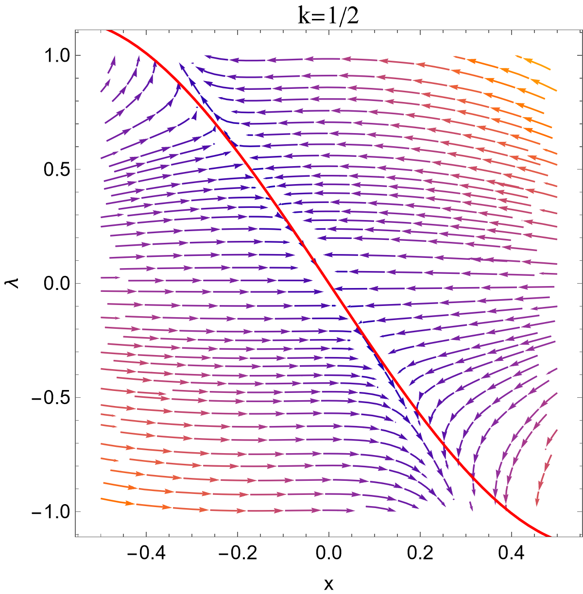
whose unit eigenvectors are $(1,0)^{\text{T}}$ and $(-1,3)^{\text{T}}/\sqrt{10}$ with respective eigenvalues $-3$ and $0$. This result means that the system evolves along $-x$ direction faster than along $(-1,3)^{\rm T}$. Such the fact suggests that the system first approaches to $x-$nucline and then is restricted on it.¹¹1In the literature of dynamical system, such a fixed point is called stable and non-isolated. In Fig. (1), we plot the solutions $(x,\lambda)$ as trajectories on the 2D plane. We see that maintaining $0\leq(\delta w=2x^{2})\ll 1$, eq. (31) amounts to the restriction of the Dark Energy trajectory to lie on the thin vertical strip centered on the $\lambda-$axis.

The evolution of $w$ can be studied in this framework. Taking derivatives of eq. (31) while taking equations (29) and (30) into account,

The equation (37) indicates that the first order derivative vanishes along the $x$-nullcline while the second order derivative (38) is small along the $x$-nullcline as long as $\lambda\ll 1$. That is to say, $\delta w$ evolves relatively slowly comparing to $\mathcal{H}$. This fact is also demonstrated in the numerical results, which are presented in Figure 2. According to the numerical results, it is clear that the change of $\delta w$ is small sufficiently long after initial time.

References

- [1] A. Ashtekar, B. Bonga, and A. Kesavan. Asymptotics with a positive cosmological constant: I. Basic framework. Classical and Quantum Gravity, 32(2):025004, 2015.
- [2] A. Ashtekar, B. Bonga, and A. Kesavan. Asymptotics with a positive cosmological constant. II. Linear fields on de Sitter spacetime. Phys. Rev. D, 92(4):044011, Aug. 2015.
- [3] A. Ashtekar, B. Bonga, and A. Kesavan. Asymptotics with a positive cosmological constant. III. The quadrupole formula. Phys. Rev. D, 92(10):104032, Nov. 2015.
- [4] J. M. Bardeen. Gauge-invariant cosmological perturbations. Phys. Rev. D, 22(8):1882–1905, Oct. 1980.
- [5] B. Bonga and J. S. Hazboun. Power radiated by a binary system in a de Sitter universe. Phys. Rev. D, 96(6):064018, Sept. 2017.
- [6] Y.-Z. Chu. Transverse traceless gravitational waves in a spatially flat FLRW universe: Causal structure from dimensional reduction. Phys. Rev. D, 92(12):124038, Dec. 2015.
- [7] Y.-Z. Chu. Gravitational wave memory in and 4D cosmology. Classical and Quantum Gravity, 34(3):035009, 2017.
- [8] Y.-Z. Chu. More on cosmological gravitational waves and their memories. Classical and Quantum Gravity, 34(19):194001, 2017.
- [9] Y.-Z. Chu and Y.-W. Liu. The transverse-traceless spin-2 gravitational wave cannot be a standalone observable because it is acausal. Classical and Quantum Gravity, 37(5):055001, 2020.
- [10] Y.-Z. Chu and Y.-W. Liu. Gravitational tensor and acoustic waves in a radiation dominated universe: Weyl curvature and polarization patterns. Phys. Rev. D, 103(12):124033, June 2021.
- [11] C. Dalang, P. Fleury, and L. Lombriser. Scalar and tensor gravitational waves. Phys. Rev. D, 103(6):064075, Mar. 2021.
- [12] H. J. de Vega, J. Ramirez, and N. Sanchez. Generation of gravitational waves by generic sources in de Sitter space-time. Phys. Rev. D, 60(4):044007, July 1999.
- [13] A. Garoffolo, G. Tasinato, C. Carbone, D. Bertacca, and S. Matarrese. Gravitational waves and geometrical optics in scalar-tensor theories. Journal of Cosmology and Astroparticle Physics, 2020(11):040, 2020.
- [14] S. J. Hoque and A. Aggarwal. Quadrupolar power radiation by a binary system in de Sitter background. International Journal of Modern Physics D, 28(01):1950025, 2019.
- [15] G. W. Horndeski. Second-order scalar-tensor field equations in a four-dimensional space. International Journal of Theoretical Physics, 10(6):363–384, 1974.
- [16] K.-i. Kubota, S. Arai, and S. Mukohyama. Propagation of scalar and tensor gravitational waves in horndeski theory. Phys. Rev. D, 107:064002, Mar 2023.
- [17] H. Nariai. On the Green’s Function in an Expanding Universe and Its Role in the Problem of Mach’s Principle. Progress of Theoretical Physics, 40(1):49–59, July 1968.
- [18] P. C. Peters and J. Mathews. Gravitational Radiation from Point Masses in a Keplerian Orbit. Phys. Rev., 131:435–440, Jul 1963.
- [19] E. Poisson and C. M. Will. Gravity: Newtonian, Post-Newtonian, Relativistic. Cambridge University Press, 2014.