Scalable regret for learning to control network-coupled subsystems with unknown dynamics

Sagar Sudhakara, Aditya Mahajan, Ashutosh Nayyar, and Yi Ouyang Sagar Sudhakara and Ashutosh Nayyar are with the Department of Electrical and Computer Engineering, University of Southern California, Los Angeles, CA, USA. (email: [email protected], [email protected])Aditya Mahajan is with the department of Electrical and Computer Engineering, McGill University, Montreal, QC, Canada. (email: [email protected])Yi Ouyang is with Preferred Networks America, Burlingame, CA, USA (email: [email protected])The work of Aditya Mahajan was supported in part by the Innovation for Defence Excellence and Security (IDEaS) Program of the Canadian Department of National Defence through grant CFPMN2-30.

Abstract

We consider the problem of controlling an unknown linear quadratic Gaussian (LQG) system consisting of multiple subsystems connected over a network. Our goal is to minimize and quantify the regret (i.e. loss in performance) of our strategy with respect to an oracle who knows the system model. Viewing the interconnected subsystems globally and directly using existing LQG learning algorithms for the global system results in a regret that increases super-linearly with the number of subsystems. Instead, we propose a new Thompson sampling based learning algorithm which exploits the structure of the underlying network. We show that the expected regret of the proposed algorithm is bounded by $\tilde{\mathcal{O}}\big{(}n\sqrt{T}\big{)}$ where $n$ is the number of subsystems, $T$ is the time horizon and the $\tilde{\mathcal{O}}(\cdot)$ notation hides logarithmic terms in $n$ and $T$ . Thus, the regret scales linearly with the number of subsystems. We present numerical experiments to illustrate the salient features of the proposed algorithm.

Index Terms:

Linear quadratic systems, networked control systems, reinforcement learning, Thompson sampling.

I Introduction

Large-scale systems comprising of multiple subsystems connected over a network arise in a number of applications including power systems, traffic networks, communication networks and some economic systems [1]. A common feature of such systems is the coupling in their subsystems’ dynamics and costs, i.e., the state evolution and local costs of one subsystem depend not only on its own state and control action but also on the states and control actions of other subsystems in the network. Analyzing various aspects of the behavior of such systems and designing control strategies for them under a variety of settings have been long-standing problems of interest in the systems and control literature [2, 3, 4, 5, 6, 7]. However, there are still many unsolved challenges, especially on the interface between learning and control in the context of these large-scale systems.

In this paper, we investigate the problem of designing control strategies for large-scale network-coupled subsystems when some parameters of the system model are not known. Due to the unknown parameters, the control problem is also a learning problem. We adopt a reinforcement learning framework for this problem with the goal of minimizing and quantifying the regret (i.e. loss in performance) of our learning-and-control strategy with respect to the optimal control strategy based on the complete knowledge of the system model.

The networked system we consider follows linear dynamics with quadratic costs and Gaussian noise. Such linear-quadratic-Gaussian (LQG) systems are one of the most commonly used modeling framework in numerous control applications. Part of the appeal of LQG models is the simple structure of the optimal control strategy when the system model is completely known—the optimal control action in this case is a linear or affine function of the state—which makes the optimal strategy easy to identify and easy to implement. If some parameters of the model are not fully known during the design phase or may change during operation, then it is better to design a strategy that learns and adapts online. Historically, both adaptive control [8] and reinforcement learning [9, 10] have been used to design asymptotically optimal learning algorithms for such LQG systems. In recent years, there has been considerable interest in analyzing the transient behavior of such algorithms which can be quantified in terms of the regret of the algorithm as a function of time. This allows one to assess, as a function of time, the performance of a learning algorithm compared to an oracle who knows the system parameters upfront.

Several learning algorithms have been proposed for LQG systems [11, 12, 13, 14, 15, 16, 17, 18, 19, 20, 21, 22, 23], and in most cases the regret is shown to be bounded by $\tilde{\mathcal{O}}(d_{x}^{0.5}(d_{x}+d_{u})\sqrt{T})$ , where $d_{x}$ is the dimension of the state, $d_{u}$ is the dimension of the controls, $T$ is the time horizon, and the $\tilde{\mathcal{O}}(\cdot)$ notation hides logarithmic terms in $T$ . Given the lower bound of $\tilde{\Omega}(d_{x}^{0.5}d_{u}\sqrt{T})$ (where $\tilde{\Omega}(\cdot)$ notation hides logarithmic terms in $T$ ) for regret in LQG systems identified in a recent work [19], the regrets of the existing algorithms have near optimal scaling in terms of time and dimension. However, when directly applied to a networked system with $n$ subsystems, these algorithms would incur $\tilde{\mathcal{O}}(n^{1.5}d_{x}^{0.5}({d_{x}+d_{u}})\sqrt{T})$ regret because the effective dimension of the state and the controls is $nd_{x}$ and $nd_{u}$ , where $d_{x}$ and $d_{u}$ are the dimensions of each subsystem. This super-linear dependence on $n$ is prohibitive in large-scale networked systems because the regret per subsystem (which is $\tilde{\mathcal{O}}(\sqrt{n})$ ) grows with the number of subsystems.

The learning algorithms mentioned above are for a general LQG system and do not take into account any knowledge of the underlying network structure. Our main contribution is to show that by exploiting the structure of the network model, it is possible to design learning algorithms for large-scale network-coupled subsystems where the regret does not grow super-linearly in the number of subsystems. In particular, we utilize a spectral decomposition technique, recently proposed in [24], to decompose the large-scale system into $L$ decoupled systems, where $L$ is the rank of the coupling matrix corresponding to the underlying network. Using the decoupled systems, we propose a Thompson sampling based algorithm with $\tilde{\mathcal{O}}(n\allowbreak d_{x}^{0.5}({d_{x}+d_{u}})\sqrt{T})$ regret bound.

Related work

Broadly speaking, three classes of low-regret learning algorithms have been proposed for LQG systems: certainty equivalence (CE) based algorithms, optimism in the face of uncertainty (OFU) based algorithms, and Thompson sampling (TS) based algorithms. CE is a classical adaptive control algorithm [8]. Recent papers [16, 17, 18, 19, 20] have established near optimal high probability bounds on regret for CE-based algorithms. OFU-based algorithms are inspired by the OFU principle for multi-armed bandits [25]. Starting with the work of [11, 12], most of the papers following the OFU approach [13, 14, 15] also provide similar high probability regret bounds. TS-based algorithms are inspired by TS algorithm for multi-armed bandits [26]. Most papers following this approach [21, 22, 23, 20] establish bounds on expected Bayesian regret of similar near-optimal orders. As argued earlier, most of these papers show that the regret scales super-linearly with the number of subsystems and are, therefore, of limited value for large-scale systems.

There is an emerging literature on learning algorithms for networked systems both for LQG models [27, 28, 29] and MDP models [30, 31, 32, 33]. The papers on LQG models propose distributed value- or policy-based learning algorithms and analyze their convergence properties, but they do not characterize their regret. Some of the papers on MDP models [32, 33] do characterize regret bounds for OFU and TS-based learning algorithms but these bounds are not directly applicable to the LQG model considered in this paper.

An important special class of network-coupled systems is mean-field coupled subsystems [34, 35]. There has been considerable interest in reinforcement learning for mean-field models [36, 37, 38], but most of the literature does not consider regret. The basic mean-field coupled model can be viewed as a special case of the network-coupled subsystems considered in this paper (see Sec. VI-A). In a preliminary version of this paper [39], we proposed a TS-based algorithm for mean-field coupled subsystems which has a $\tilde{\mathcal{O}}((1+1/n)\sqrt{T})$ regret per subsystem. The current paper extends the TS-based algorithm to general network-coupled subsystems and establishes scalable regret bounds for arbitrarily coupled networks.

Organization

The rest of the paper is organized as follows. In Section II, we introduce the model of network-coupled subsystems. In Section III, we summarize the spectral decomposition idea and the resulting scalable method for synthesizing optimal control strategy when the model parameters are known. Then, in Section IV, we consider the learning problem for unknown network-coupled subsystems and present a TS-based learning algorithm with scalable regret bound. We subsequently provide regret analysis in Section V and numerical experiments in Section VI. We conclude in Section VII.

Notation

The notation $A=[a^{ij}]$ means that $a^{ij}$ is the $(i,j)$ th element of the matrix $A$ . For a matrix $A$ , $A^{\mathchoice{\raisebox{0.0pt}{$\displaystyle\intercal$}}{\raisebox{0.0pt}{$\textstyle\intercal$}}{\raisebox{0.0pt}{$\scriptstyle\intercal$}}{\raisebox{0.0pt}{$\scriptscriptstyle\intercal$}}}$ denotes its transpose. Given matrices (or vectors) $A_{1}$ , …, $A_{n}$ with the same number of rows, $[A_{1},\dots,A_{n}]$ denotes the matrix formed by horizontal concatenation. For a random vector $v$ , $\operatorname{var}(v)$ denotes its covariance matrix. The notation $\mathcal{N}(\mu,\Sigma)$ denotes the multivariate Gaussian distribution with mean vector $\mu$ and covariance matrix $\Sigma$ .

For stabilizable $(A,B)$ and positive definite matrices $Q,R$ , DARE $(A,B,Q,R)$ denotes the unique positive semidefinite solution of the discrete time algebraic Riccati equation (DARE), which is given as

S=A^{\mathchoice{\raisebox{0.0pt}{$\displaystyle\intercal$}}{\raisebox{0.0pt}{$\textstyle\intercal$}}{\raisebox{0.0pt}{$\scriptstyle\intercal$}}{\raisebox{0.0pt}{$\scriptscriptstyle\intercal$}}}SA-(A^{\mathchoice{\raisebox{0.0pt}{$\displaystyle\intercal$}}{\raisebox{0.0pt}{$\textstyle\intercal$}}{\raisebox{0.0pt}{$\scriptstyle\intercal$}}{\raisebox{0.0pt}{$\scriptscriptstyle\intercal$}}}SB)(R+B^{\mathchoice{\raisebox{0.0pt}{$\displaystyle\intercal$}}{\raisebox{0.0pt}{$\textstyle\intercal$}}{\raisebox{0.0pt}{$\scriptstyle\intercal$}}{\raisebox{0.0pt}{$\scriptscriptstyle\intercal$}}}SB)^{-1}(B^{\mathchoice{\raisebox{0.0pt}{$\displaystyle\intercal$}}{\raisebox{0.0pt}{$\textstyle\intercal$}}{\raisebox{0.0pt}{$\scriptstyle\intercal$}}{\raisebox{0.0pt}{$\scriptscriptstyle\intercal$}}}SA)+Q.

II Model of network-coupled subsystems

We start by describing a minor variation of a model of network-coupled subsystems proposed in [24]. The model in [24] was described in continuous time. We translate the model and the results to discrete time.

II-A System model

II-A1 Graph stucture

Consider a network consisting of $n$ subsystems/agents connected over an undirected weighted graph denoted by $\mathcal{G}(N,E,W_{\mathcal{G}})$ , where $N=\{1,\dots,n\}$ is the set of nodes, $E\subseteq N\times N$ is the set of edges, and $W_{\mathcal{G}}=[w^{ij}]\in\mathds{R}^{n\times n}$ is the weighted adjacency matrix. Let $M=[m^{ij}]\in\mathds{R}^{n\times n}$ be a symmetric coupling matrix corresponding to the underlying graph $\mathcal{G}$ . For instance, $M$ may represent the underlying adjacency matrix (i.e., $M=W_{\mathcal{G}}$ ) or the underlying Laplacian matrix (i.e., $M=\operatorname{diag}(W_{\mathcal{G}}\mathds{1}_{n})-W_{\mathcal{G}}$ ).

II-A2 State and dynamics

The states and control actions of agents take values in $\mathds{R}^{d_{x}}$ and $\mathds{R}^{d_{u}}$ , respectively. For agent $i\in N$ , we use $x^{i}_{t}\in\mathds{R}^{d_{x}}$ and $u^{i}_{t}\in\mathds{R}^{d_{u}}$ to denote its state and control action at time $t$ .

The system starts at a random initial state $x_{1}=(x^{i}_{1})_{i\in N}$ , whose components are independent across agents. For agent $i$ , the initial state $x^{i}_{1}\sim\mathcal{N}(0,\Xi^{i}_{1})$ , and at any time $t\geq 1$ , the state evolves according to

x^{i}_{t+1}=Ax^{i}_{t}+Bu^{i}_{t}+Dx^{\mathcal{G},i}_{t}+Eu^{\mathcal{G},i}_{t}+w^{i}_{t},

(1)

where $x^{\mathcal{G},i}_{t}$ and $u^{\mathcal{G},i}_{t}$ are the locally perceived influence of the network on the state of agent $i$ and are given by

x^{\mathcal{G},i}_{t}=\sum_{j\in N}m^{ij}x^{j}_{t}\quad\text{and}\quad u^{\mathcal{G},i}_{t}=\sum_{j\in N}m^{ij}u^{j}_{t},

(2)

$A$ , $B$ , $D$ , $E$ are matrices of appropriate dimensions, and $\{w^{i}_{t}\}_{t\geq 1},i\in N,$ are i.i.d. zero-mean Gaussian processes which are independent of each other and the initial state. In particular, $w^{i}_{t}\in\mathds{R}^{d_{x}}$ and $w^{i}_{t}\sim\mathcal{N}(0,W)$ . We call $x^{\mathcal{G},i}_{t}$ and $u^{\mathcal{G},i}_{t}$ the network-field of the states and control actions at node $i$ at time $t$ .

Thus, the next state of agent $i$ depends on its current local state and control action, the current network-field of the states and control actions of the system, and the current local noise.

We follow the same atypical representation of the “vectorized” dynamics as used in [24]. Define $x_{t}$ and $u_{t}$ as the global state and control actions of the system:

x_{t}=[x^{1}_{t},\dots.,x^{n}_{t}]\quad\text{and}\quad u_{t}=[u^{1}_{t},\dots.,u^{n}_{t}].

We also define $w_{t}=[w^{1}_{t},\dots.,w^{n}_{t}]$ . Similarly, define $x^{\mathcal{G}}_{t}$ and $u^{\mathcal{G}}_{t}$ as the global network field of states and actions:

x^{\mathcal{G}}_{t}=[x^{\mathcal{G},1}_{t},\dots.,x^{\mathcal{G},n}_{t}]\quad\text{and}\quad u^{\mathcal{G}}_{t}=[u^{\mathcal{G},1}_{t},\dots.,u^{\mathcal{G},n}_{t}].

Note that $x_{t},x^{\mathcal{G}}_{t},w_{t}\in\mathbb{R}^{d_{x}\times n}$ and $u_{t},u^{\mathcal{G}}_{t}\in\mathbb{R}^{d_{u}\times n}$ are matrices and not vectors. The global system dynamics may be written as:

x_{t+1}=Ax_{t}+Bu_{t}+Dx^{\mathcal{G}}_{t}+Eu^{\mathcal{G}}_{t}+w_{t}.

(3)

Furthermore, we may write

x^{\mathcal{G}}_{t}=x_{t}M^{\mathchoice{\raisebox{0.0pt}{$\displaystyle\intercal$}}{\raisebox{0.0pt}{$\textstyle\intercal$}}{\raisebox{0.0pt}{$\scriptstyle\intercal$}}{\raisebox{0.0pt}{$\scriptscriptstyle\intercal$}}}=x_{t}M\quad\text{and}\quad u^{\mathcal{G}}_{t}=u_{t}M^{\mathchoice{\raisebox{0.0pt}{$\displaystyle\intercal$}}{\raisebox{0.0pt}{$\textstyle\intercal$}}{\raisebox{0.0pt}{$\scriptstyle\intercal$}}{\raisebox{0.0pt}{$\scriptscriptstyle\intercal$}}}=u_{t}M.

II-A3 Per-step cost

At any time $t$ the system incurs a per-step cost given by

c(x_{t},u_{t})=\sum_{i\in N}\sum_{j\in N}[h_{x}^{ij}(x^{i}_{t})^{\mathchoice{\raisebox{0.0pt}{$\displaystyle\intercal$}}{\raisebox{0.0pt}{$\textstyle\intercal$}}{\raisebox{0.0pt}{$\scriptstyle\intercal$}}{\raisebox{0.0pt}{$\scriptscriptstyle\intercal$}}}Q(x^{j}_{t})+h_{u}^{ij}(u^{i}_{t})^{\mathchoice{\raisebox{0.0pt}{$\displaystyle\intercal$}}{\raisebox{0.0pt}{$\textstyle\intercal$}}{\raisebox{0.0pt}{$\scriptstyle\intercal$}}{\raisebox{0.0pt}{$\scriptscriptstyle\intercal$}}}R(u^{j}_{t})]

(4)

where $Q$ and $R$ are matrices of appropriate dimensions and $h_{x}^{ij}$ and $h_{u}^{ij}$ are real valued weights. Let $H_{x}=[h_{x}^{ij}]$ and $H_{u}=[h_{u}^{ij}]$ . It is assumed that the weight matrices $H_{x}$ and $H_{u}$ are polynomials of $M$ , i.e.,

H_{x}=\sum_{k=0}^{K_{x}}q_{k}M^{k}\quad\text{and}\quad H_{u}=\sum_{k=0}^{K_{u}}r_{k}M^{k}

(5)

where $K_{x}$ and $K_{u}$ denote the degrees of the polynomials and $\{q_{k}\}^{K_{x}}_{k=0}$ and $\{r_{k}\}_{k=0}^{K_{u}}$ are real-valued coefficients.

The assumption that $H_{x}$ and $H_{u}$ are polynomials of $M$ captures the intuition that the per-step cost respects the graph structure. In the special case when $H_{x}=H_{u}=I$ , the per-step cost is decoupled across agents. When $H_{x}=H_{u}=I+M$ , the per-step cost captures a cross-coupling between one-hop neighbors. Similarly, when $H_{u}=I+M+M^{2}$ , the per-step cost captures a cross-coupling between one- and two-hop neighbors. See [24] for more examples of special cases of the per-step cost defined above.

II-B Assumptions on the model

Since $M$ is real and symmetric, it has real eigenvalues. Let $L$ denote the rank of $M$ and $\lambda^{1},\dots.,\lambda^{L}$ denote the non-zero eigenvalues. For ease of notation, for $\ell\in{1,\dots,L}$ , define

q^{\ell}=\sum_{k=0}^{K_{x}}q_{k}(\lambda^{\ell})^{k}\quad\text{and}\quad r^{\ell}=\sum_{k=0}^{K_{u}}r_{k}(\lambda^{\ell})^{k},

where $\{q_{k}\}^{K_{x}}_{k=0}$ and $\{r_{k}\}^{K_{u}}_{k=0}$ are the coefficients in (5). Furthermore, for $\ell\in\{1,\dots,L\}$ , define:

A^{\ell}={A}+\lambda^{\ell}{D}\quad\text{and}\quad B^{\ell}={B}+\lambda^{\ell}{E}.

We impose the following assumptions:

(A1): The systems $(A,B)$ and $\{(A^{\ell},B^{\ell})\}_{\ell=1}^{L}$ are stabilizable.
(A2): The matrices $Q$ and $R$ are symmetric and positive definite.
(A3): The parameters $q_{0}$ , $r_{0}$ , $\{q^{\ell}\}_{\ell=1}^{L}$ , and $\{r^{\ell}\}_{\ell=1}^{L}$ are strictly positive.

Assumption (A1) is a standard assumption. Assumptions (A2) and (A3) ensure that the per-step cost is strictly positive.

II-C Admissible policies and performance criterion

There is a system operator who has access to the state and action histories of all agents and who selects the agents’ control actions according to a deterministic or randomized (and potentially history-dependent) policy

u_{t}=\pi_{t}(x_{1:t},u_{1:t-1}).

(6)

Let $\theta^{\mathchoice{\raisebox{0.0pt}{$\displaystyle\intercal$}}{\raisebox{0.0pt}{$\textstyle\intercal$}}{\raisebox{0.0pt}{$\scriptstyle\intercal$}}{\raisebox{0.0pt}{$\scriptscriptstyle\intercal$}}}=[A,B,D,E]$ denote the parameters of the system dynamics. The performance of any policy $\pi=(\pi_{1},\pi_{2},\dots)$ is measured by the long-term average cost given by

J(\pi;\theta)=\limsup_{T\to\infty}\frac{1}{T}\mathbb{E}^{\pi}\biggl{[}\sum_{t=1}^{T}c(x_{t},u_{t})\biggr{]}.

(7)

Let $J(\theta)$ denote the minimum of $J(\pi;\theta)$ over all policies.

We are interested in the setup where the graph coupling matix $M$ , the cost coupling matrices $H_{x}$ and $H_{u}$ , and the cost matrices $Q$ and $R$ are known but the system dynamics $\theta$ are unknown and there is a prior distribution on $\theta$ . The Bayesian regret of a policy $\pi$ operating for a horizon $T$ is defined as

R(T;\pi)\coloneqq\mathbb{E}^{\pi}\biggl{[}\sum_{t=1}^{T}c(x_{t},u_{t})-TJ(\theta)\biggr{]},

(8)

where the expectation is with respect to the prior on $\theta$ , the noise processes, the initial conditions, and the potential randomizations done by the policy $\pi$ .

III Background on spectral decomposition of the system

In this section, we summarize the main results of [24], translated to the discrete-time model used in this paper.

The spectral decomposition described in [24] relies on the spectral factorization of the graph coupling matrix $M$ . Since $M$ is a real and symmetric matrix with rank $L$ , we can write it as

M=\sum_{\ell=1}^{L}\lambda^{\ell}v^{\ell}(v^{\ell})^{\mathchoice{\raisebox{0.0pt}{$\displaystyle\intercal$}}{\raisebox{0.0pt}{$\textstyle\intercal$}}{\raisebox{0.0pt}{$\scriptstyle\intercal$}}{\raisebox{0.0pt}{$\scriptscriptstyle\intercal$}}},

(9)

where $(\lambda^{1},\dots,\lambda^{L})$ are the non-zero eigenvalues of $M$ and $(v^{1},\dots,v^{L})$ are the corresponding orthonormal eigenvectors.

We now present the decomposition of the dynamics and the cost based on (9) as described in [24].

III-A Spectral decomposition of the dynamics and per-step cost

For $\ell\in\{1,2,\dots,L\}$ , define eigenstates and eigencontrols as

x^{\ell}_{t}=x_{t}v^{\ell}(v^{\ell})^{\mathchoice{\raisebox{0.0pt}{$\displaystyle\intercal$}}{\raisebox{0.0pt}{$\textstyle\intercal$}}{\raisebox{0.0pt}{$\scriptstyle\intercal$}}{\raisebox{0.0pt}{$\scriptscriptstyle\intercal$}}}\quad\text{and}\quad u^{\ell}_{t}=u_{t}v^{\ell}(v^{\ell})^{\mathchoice{\raisebox{0.0pt}{$\displaystyle\intercal$}}{\raisebox{0.0pt}{$\textstyle\intercal$}}{\raisebox{0.0pt}{$\scriptstyle\intercal$}}{\raisebox{0.0pt}{$\scriptscriptstyle\intercal$}}},

(10)

respectively. Furthermore, define auxiliary state and auxiliary control as

\breve{x}_{t}=x_{t}-\sum_{\ell=1}^{L}x^{\ell}_{t}\quad\text{and}\quad\breve{u}_{t}=u_{t}-\sum_{\ell=1}^{L}u^{\ell}_{t},

(11)

respectively. Similarly, define $w^{\ell}_{t}=w_{t}v^{\ell}(v^{\ell})^{\mathchoice{\raisebox{0.0pt}{$\displaystyle\intercal$}}{\raisebox{0.0pt}{$\textstyle\intercal$}}{\raisebox{0.0pt}{$\scriptstyle\intercal$}}{\raisebox{0.0pt}{$\scriptscriptstyle\intercal$}}}$ and $\breve{w}_{t}=w_{t}-\sum_{\ell=1}^{L}w^{\ell}_{t}$ . Let $x^{\ell,i}_{t}$ and $u^{\ell,i}_{t}$ denote the $i$ -th column of $x^{\ell}_{t}$ and $u^{\ell}_{t}$ respectively; thus we can write

x^{\ell}_{t}=[x^{\ell,1}_{t},\dots.,x^{\ell,n}_{t}]\quad\text{and}\quad u^{\ell}_{t}=[u^{\ell,1}_{t},\dots.,u^{\ell,n}_{t}].

Similar interpretations hold for $w^{\ell,i}_{t}$ and $\breve{w}^{i}_{t}$ . Following [24, Lemma 2], we can show that for any $i\in N$ ,

\operatorname{var}(w^{\ell,i}_{t})=(v^{\ell,i})^{2}W\quad\text{and}\quad\operatorname{var}(\breve{w}^{i}_{t})=(\breve{v}^{i})^{2}W,

(12)

where $(\breve{v}^{i})^{2}=1-\sum_{\ell=1}^{L}(v^{\ell,i})^{2}$ . These covariances do not depend on time because the noise processes are i.i.d.

Using the same argument as in [24, Propositions 1 and 2], we can show the following.

Proposition 1

For each node $i\in N$ , the state and control action may be decomposed as

x^{i}_{t}=\breve{x}^{i}_{t}+\sum_{\ell=1}^{L}x^{\ell,i}_{t}\quad\text{and}\quad u^{i}_{t}=\breve{u}^{i}_{t}+\sum_{\ell=1}^{L}u^{\ell,i}_{t}

(13)

where the dynamics of eigenstate $x^{\ell,i}_{t}$ depend only on $u^{\ell,i}_{t}$ and $w^{\ell,i}_{t}$ , and are given by

x^{\ell,i}_{t+1}=(A+\lambda^{\ell}D)x^{\ell,i}_{t}+(B+\lambda^{\ell}E)u^{\ell,i}_{t}+w^{\ell,i}_{t},

(14)

and the dynamics of the auxiliary state $\breve{x}^{i}_{t}$ depend only on $\breve{u}^{i}_{t}$ and $\breve{w}^{i}_{t}$ and are given by

\breve{x}^{i}_{t+1}=A\breve{x}^{i}_{t}+B\breve{u}^{i}_{t}+\breve{w}^{i}_{t}.

(15)

Furthermore, the per-step cost decomposes as follows:

c(x_{t},u_{t})=\sum_{i\in N}\biggl{[}q_{0}\breve{c}(\breve{x}^{i}_{t},\breve{u}^{i}_{t})+\sum_{\ell=1}^{L}q^{\ell}c^{\ell}(x^{\ell,i}_{t},u^{\ell,i}_{t})\biggr{]}

(16)

where¹¹1Recall that (A3) ensures that $q_{0}$ and $\{q^{\ell}\}_{\ell=1}^{L}$ are strictly positive.

	$\displaystyle\breve{c}(\breve{x}^{i}_{t},\breve{u}^{i}_{t})$	$\displaystyle=({\breve{x}^{i}_{t}})^{\mathchoice{\raisebox{0.0pt}{$\displaystyle\intercal$}}{\raisebox{0.0pt}{$\textstyle\intercal$}}{\raisebox{0.0pt}{$\scriptstyle\intercal$}}{\raisebox{0.0pt}{$\scriptscriptstyle\intercal$}}}Q\breve{x}^{i}_{t}+\frac{r_{0}}{q_{0}}({\breve{u}^{i}_{t}})^{\mathchoice{\raisebox{0.0pt}{$\displaystyle\intercal$}}{\raisebox{0.0pt}{$\textstyle\intercal$}}{\raisebox{0.0pt}{$\scriptstyle\intercal$}}{\raisebox{0.0pt}{$\scriptscriptstyle\intercal$}}}R\breve{u}^{i}_{t},$
	$\displaystyle c^{\ell}(x^{\ell,i}_{t},u^{\ell,i}_{t})$	$\displaystyle=(x^{\ell,i}_{t})^{\mathchoice{\raisebox{0.0pt}{$\displaystyle\intercal$}}{\raisebox{0.0pt}{$\textstyle\intercal$}}{\raisebox{0.0pt}{$\scriptstyle\intercal$}}{\raisebox{0.0pt}{$\scriptscriptstyle\intercal$}}}Qx^{\ell,i}_{t}+\frac{r^{\ell}}{q^{\ell}}(u^{\ell,i}_{t})^{\mathchoice{\raisebox{0.0pt}{$\displaystyle\intercal$}}{\raisebox{0.0pt}{$\textstyle\intercal$}}{\raisebox{0.0pt}{$\scriptstyle\intercal$}}{\raisebox{0.0pt}{$\scriptscriptstyle\intercal$}}}Ru^{\ell,i}_{t}.$

_□

III-B Planning solution for network-coupled subsystems

We now present the main result of [24], which provides a scalable method to synthesize the optimal control policy when the system dynamics are known.

Based on Proposition 1, we can view the overall system as the collection of the following subsystems:

•

Eigen-system $(\ell,i)$ , $\ell\in\{1,\dots,L\}$ and $i\in N$ with state $x^{\ell,i}_{t}$ , controls $u^{\ell,i}_{t}$ , dynamics (14), and per-step cost $q^{\ell}c^{\ell}(x^{\ell,i},u^{\ell,i})$ .
•

Auxiliary system $i$ , $i\in N$ , with state $\breve{x}^{i}_{t}$ , controls $\breve{u}^{i}_{t}$ , dynamics (15), and per-step cost $\breve{q}_{0}\breve{c}(\breve{x}^{i}_{t},\breve{u}^{i}_{t})$ .

Let $(\theta^{\ell})^{\mathchoice{\raisebox{0.0pt}{$\displaystyle\intercal$}}{\raisebox{0.0pt}{$\textstyle\intercal$}}{\raisebox{0.0pt}{$\scriptstyle\intercal$}}{\raisebox{0.0pt}{$\scriptscriptstyle\intercal$}}}=[A^{\ell},B^{\ell}]\coloneqq[(A+\lambda^{\ell}D),(B+\lambda^{\ell}E)]$ , $\ell\in\{1,\dots,L\}$ , and $\breve{\theta}^{\mathchoice{\raisebox{0.0pt}{$\displaystyle\intercal$}}{\raisebox{0.0pt}{$\textstyle\intercal$}}{\raisebox{0.0pt}{$\scriptstyle\intercal$}}{\raisebox{0.0pt}{$\scriptscriptstyle\intercal$}}}=[A,B]$ denote the parameters of the dynamics of the eigen and auxiliary systems, respectively. Then, for any policy $\pi=(\pi_{1},\pi_{2},\dots)$ , the performance of the eigensystem $(\ell,i)$ , $\ell\in\{1,\dots,L\}$ and $i\in N$ , is given by $q^{\ell}J^{\ell,i}(\pi;\theta^{\ell})$ , where

J^{\ell,i}(\pi;\theta^{\ell})=\limsup_{T\to\infty}\frac{1}{T}\mathbb{E}^{\pi}\biggl{[}\sum_{t=1}^{T}c(x^{\ell,i}_{t},u^{\ell,i}_{t})\biggr{]}.

Similarly, the performance of the auxiliary system $i$ , $i\in N$ , is given by $\breve{q}_{0}\breve{J}^{i}(\pi;\breve{\theta})$ , where

\breve{J}^{i}(\pi;\breve{\theta})=\limsup_{T\to\infty}\frac{1}{T}\mathbb{E}^{\pi}\biggl{[}\sum_{t=1}^{T}c(\breve{x}^{i}_{t},\breve{u}^{i}_{t})\biggr{]}.

Proposition 1 implies that the overall performance of policy $\pi$ can be decomposed as

J(\pi;\theta)=\sum_{i\in N}q_{0}\breve{J}^{i}(\pi;\breve{\theta})+\sum_{i\in N}\sum_{\ell=1}^{L}q^{\ell}J^{\ell,i}(\pi;\theta^{\ell}).

(17)

The key intuition behind the result of [24] is as follows. By the certainty equivalence principle for LQ systems, we know that (when the system dynamics are known) the optimal control policy of a stochastic LQ system is the same as the optimal control policy of the corresponding deterministic LQ system where the noises $\{w^{i}_{t}\}_{t\geq 1}$ are assumed to be zero. Note that when noises $\{w^{i}_{t}\}_{t\geq 1}$ are zero, then the noises $\{w^{\ell,i}_{t}\}_{t\geq 1}$ and $\{\breve{w}^{i}_{t}\}_{t\geq 1}$ of the eigen- and auxiliary-systems are also zero. This, in turn, implies that the dynamics of all the eigen- and auxiliary systems are decoupled. These decoupled dynamics along with the cost decoupling in (17) imply that we can choose the controls $\{u^{\ell,i}_{t}\}_{t\geq 1}$ for the eigensystem $(\ell,i)$ , $\ell\in\{1,\dots,L\}$ and $i\in N$ , to minimize²²2The cost of the eigensystem $(\ell,i)$ is $q^{\ell}J^{\ell,i}(\pi;\theta^{\ell})$ . From (A3), we know that $q^{\ell}$ is positive. Therefore, minimizing $q^{\ell}J^{\ell,i}(\pi;\theta^{\ell})$ is the same as minimizing $J^{\ell,i}(\pi;\theta^{\ell})$ . $J^{\ell,i}(\pi;\theta^{\ell})$ and choose the controls $\{\breve{u}^{i}_{t}\}_{t\geq 1}$ for the auxiliary system $i$ , $i\in N$ , to minimize³³3The same remark as footnote 2 applies here. $\breve{J}^{i}(\pi;\breve{\theta})$ . These optimization problems are standard optimal control problems. Therefore, similar to [24, Thoerem 3], we obtain the following result.

Theorem 1

Let $\breve{{S}}$ and $\{S^{\ell}\}_{\ell=1}^{L}$ be the solution of the following discrete time algebraic Riccati equations (DARE):


	$\displaystyle\breve{{S}}(\breve{\theta})$	$\displaystyle=\operatorname{DARE}(A,B,Q,\tfrac{r_{0}}{q_{0}}R),$	(18a)
and for $\ell\in\{1,\dots,L\}$ ,
	$\displaystyle S^{\ell}(\theta^{\ell})$	$\displaystyle=\operatorname{DARE}(A^{\ell},B^{\ell},Q,\tfrac{r^{\ell}}{q^{\ell}}R).$	(18b)

Define the gains:


	$\displaystyle\breve{{G}}(\breve{\theta})$	$\displaystyle=-\bigl{(}(B)^{\mathchoice{\raisebox{0.0pt}{$\displaystyle\intercal$}}{\raisebox{0.0pt}{$\textstyle\intercal$}}{\raisebox{0.0pt}{$\scriptstyle\intercal$}}{\raisebox{0.0pt}{$\scriptscriptstyle\intercal$}}}\breve{{S}}(\breve{\theta})B+\tfrac{r_{0}}{q_{0}}R\bigr{)}^{-1}(B)^{\mathchoice{\raisebox{0.0pt}{$\displaystyle\intercal$}}{\raisebox{0.0pt}{$\textstyle\intercal$}}{\raisebox{0.0pt}{$\scriptstyle\intercal$}}{\raisebox{0.0pt}{$\scriptscriptstyle\intercal$}}}\breve{{S}}(\breve{\theta})A,$	(19a)
and for $\ell\in\{1,\dots,L\}$ ,
	$\displaystyle G^{\ell}(\theta^{\ell})$	$\displaystyle=-\bigl{(}(B^{\ell})^{\mathchoice{\raisebox{0.0pt}{$\displaystyle\intercal$}}{\raisebox{0.0pt}{$\textstyle\intercal$}}{\raisebox{0.0pt}{$\scriptstyle\intercal$}}{\raisebox{0.0pt}{$\scriptscriptstyle\intercal$}}}S^{\ell}(\theta^{\ell})B^{\ell}+\tfrac{r^{\ell}}{q^{\ell}}R\bigr{)}^{-1}(B^{\ell})^{\mathchoice{\raisebox{0.0pt}{$\displaystyle\intercal$}}{\raisebox{0.0pt}{$\textstyle\intercal$}}{\raisebox{0.0pt}{$\scriptstyle\intercal$}}{\raisebox{0.0pt}{$\scriptscriptstyle\intercal$}}}S^{\ell}(\theta^{\ell})A^{\ell}.$	(19b)

Then, under assumptions (A1)–(A3), the policy

u^{i}_{t}=\breve{{G}}(\breve{\theta})\breve{x}^{i}_{t}+\sum_{\ell=1}^{L}G^{\ell}(\theta^{\ell})x^{\ell,i}_{t}

(20)

minimizes the long-term average cost in (7) over all admissible policies. Furthermore, the optimal performance is given by

J(\theta)=\sum_{i\in N}q_{0}\breve{J}^{i}(\breve{\theta})+\sum_{i\in N}\sum_{\ell=1}^{L}q^{\ell}J^{\ell,i}(\theta^{\ell}),

(21)

where

\breve{J}^{i}(\breve{\theta})=(\breve{v}^{i})^{2}\operatorname{Tr}(W\breve{{S}})

(22)

and for $\ell\in\{1,\dots,L\}$ ,

J^{\ell,i}(\theta^{\ell})=(v^{\ell,i})^{2}\operatorname{Tr}(WS^{\ell}).

(23)

_□

IV Learning for network-coupled subsystems

For the ease of notation, we define $z^{\ell,i}_{t}=\operatorname{vec}(x^{\ell,i}_{t},u^{\ell,i}_{t})$ and $\breve{z}^{i}_{t}=\operatorname{vec}(\breve{x}^{i}_{t},\breve{u}^{i}_{t})$ . Then, we can write the dynamics (14), (15) of the eigen and the auxiliary systems as


$\displaystyle{x}^{\ell,i}_{t+1}$	$\displaystyle=(\theta^{\ell})^{\mathchoice{\raisebox{0.0pt}{$\displaystyle\intercal$}}{\raisebox{0.0pt}{$\textstyle\intercal$}}{\raisebox{0.0pt}{$\scriptstyle\intercal$}}{\raisebox{0.0pt}{$\scriptscriptstyle\intercal$}}}{z}^{\ell,i}_{t}+w^{\ell,i}_{t},$	$\displaystyle\forall i\in N,\forall\ell\in\{1,\dots,L\},$	(24a)
$\displaystyle\breve{x}^{i}_{t+1}$	$\displaystyle=(\breve{\theta})^{\mathchoice{\raisebox{0.0pt}{$\displaystyle\intercal$}}{\raisebox{0.0pt}{$\textstyle\intercal$}}{\raisebox{0.0pt}{$\scriptstyle\intercal$}}{\raisebox{0.0pt}{$\scriptscriptstyle\intercal$}}}\breve{z}^{i}_{t}+\breve{w}^{i}_{t},$	$\displaystyle\forall i\in N.$	(24b)

IV-A Simplifying assumptions

We impose the following assumptions to simplify the description of the algorithm and the regret analysis.

(A4): The noise covariance $W$ is a scaled identity matrix given by $\sigma_{w}^{2}I$ .
(A5): For each $i\in N$ , $\breve{v}^{i}\neq 0$ .

Assumption (A4) is commonly made in most of the literature on regret analysis of LQG systems. An implication of (A4) is that $\operatorname{var}(\breve{w}^{i}_{t})=(\breve{\sigma}^{i})^{2}I$ and $\operatorname{var}(w^{\ell,i}_{t})=(\sigma^{\ell,i})^{2}I$ , where

(\breve{\sigma}^{i})^{2}=(\breve{v}^{i})^{2}\sigma_{w}^{2}\quad\text{and}\quad(\sigma^{\ell,i})^{2}=(v^{\ell,i})^{2}\sigma_{w}^{2}.

(25)

Assumption (A5) is made to rule out the case where the dynamics of some of the auxiliary systems are deterministic.

IV-B Prior and posterior beliefs:

We assume that the unknown parameters $\breve{\theta}$ and $\{\theta^{\ell}\}_{\ell=1}^{L}$ lie in compact subsets $\breve{\Theta}$ and $\{\Theta^{\ell}\}_{\ell=1}^{L}$ of $\mathds{R}^{(d_{x}+d_{u})\times d_{x}}$ . Let $\breve{\theta}^{k}$ denote the $k$ -th column of $\breve{\theta}$ . Thus $\breve{\theta}=[\breve{\theta}^{1},\dots,\breve{\theta}^{d_{x}}]$ . Similarly, let $\theta^{\ell,k}$ denote the $k$ -th column of $\theta^{\ell}$ . Thus, $\theta^{\ell}=[\theta^{\ell,1},\dots,\theta^{\ell,d_{x}}]$ . We use $p\bigr{|}_{\Theta}$ to denote the restriction of probability distribution $p$ on the set $\Theta$ .

We assume that $\breve{\theta}$ and $\{\theta^{\ell}\}_{\ell=1}^{L}$ are random variables that are independent of the initial states and the noise processes. Furthermore, we assume that the priors $\breve{p}_{1}$ and $\{p^{\ell}_{1}\}_{\ell=1}^{L}$ on $\breve{\theta}$ and $\{\theta^{\ell}\}_{\ell=1}^{L}$ , respectively, satisfy the following:

(A6)

$\breve{p}_{1}$ is given as:

\breve{p}_{1}(\breve{\theta})=\biggl{[}\prod_{k=1}^{d_{x}}\breve{\xi}^{k}_{1}(\breve{\theta}^{k})\biggr{]}\biggr{|}_{\breve{\Theta}}

where for $k\in\{1,\dots,d_{x}\}$ , $\breve{\xi}_{1}^{k}=\mathcal{N}(\breve{\mu}_{1}^{k},\breve{\Sigma}_{1})$ with mean $\breve{\mu}_{1}^{k}\in\mathds{R}^{d_{x}+d_{u}}$ and positive-definite covariance $\breve{\Sigma}_{1}\in\mathds{R}^{(d_{x}+d_{u})\times(d_{x}+d_{u})}$ .

(A7)

For each $\ell\in\{1,\dots,L\}$ , $p^{\ell}_{1}$ is given as:

p^{\ell}_{1}(\theta^{\ell})=\biggl{[}\prod_{k=1}^{d_{x}}{\xi}^{\ell,k}_{1}(\theta^{\ell,k})\biggr{]}\biggr{|}_{\Theta^{\ell}}

where for $k\in\{1,\dots,d_{x}\}$ , $\xi_{1}^{\ell,k}=\mathcal{N}(\mu^{\ell,k}_{1},\Sigma^{\ell}_{1})$ with mean $\mu^{\ell,k}_{1}\in\mathds{R}^{(d_{x}+d_{u})}$ and positive-definite covariance $\Sigma^{\ell}_{1}\in\mathds{R}^{(d_{x}+d_{u})\times(d_{x}+d_{u})}$ .

These assumptions are similar to the assumptions on the prior in the recent literature on Thompson sampling for LQ systems [21, 22].

Our learning algorithm (and TS-based algorithms in general) keeps track of a posterior distribution on the unknown parameters based on observed data. Motivated by the nature of the planning solution (see Theorem 1), we maintain separate posterior distributions on $\breve{\theta}$ and $\{\theta^{\ell}\}_{\ell=1}^{L}$ . For each $\ell$ , we select an subsystem $i^{\ell}_{*}$ such that the $i^{\ell}_{*}$ -th component of the eigen-vector $v^{\ell}$ is non-zero (i.e. $v^{\ell,i^{\ell}_{*}}\neq 0$ ) . At time $t$ , we maintain a posterior distribution $p^{\ell}_{t}$ on $\theta^{\ell}$ based on the corresponding eigen state and action history of the $i^{\ell}_{*}$ -th subsystem. In other words, for any Borel subset $B$ of $\mathds{R}^{(d_{x}+d_{u})\times d_{x}}$ , $p^{\ell}_{t}(B)$ gives the following conditional probability

p^{\ell}_{t}(B)=\mathds{P}(\theta^{\ell}\in B\mid x^{\ell,i^{\ell}_{*}}_{1:t},u^{\ell,i^{\ell}_{*}}_{1:t-1}).

(26)

We maintain a separate posterior distribution $\breve{p}_{t}$ on $\breve{\theta}$ as follows. At each time $t>1$ , we select an subsystem $j_{t-1}=\arg\max_{i\in N}\breve{z}^{i^{\mathchoice{\raisebox{0.0pt}{$\displaystyle\intercal$}}{\raisebox{0.0pt}{$\textstyle\intercal$}}{\raisebox{0.0pt}{$\scriptstyle\intercal$}}{\raisebox{0.0pt}{$\scriptscriptstyle\intercal$}}}}_{t-1}\breve{\Sigma}_{t-1}\breve{z}^{i}_{t-1}/(\breve{\sigma}^{i}_{t})^{2}$ , where $\breve{\Sigma}_{t-1}$ is a covariance matrix defined recursively in Lemma 1 below. Then, for any Borel subset $B$ of $\mathds{R}^{(d_{x}+d_{u})\times d_{x}}$ ,

\breve{p}_{t}(B)=\mathds{P}(\breve{\theta}\in B\mid\{\breve{x}^{j_{s}}_{s},\breve{u}^{j_{s}}_{s},\breve{x}^{j_{s}}_{s+1}\}_{1\leq s<t}\}),

(27)

See [39] for a discussion on the rule to select $j_{t-1}$ .

Lemma 1

The posterior distributions $p^{\ell}_{t}$ , $\ell\in\{1,2,\dots,L\}$ , and $\breve{p}_{t}$ are given as follows:

$p^{\ell}_{1}$ is given by Assumption (A7) and for any $t\geq 1$ ,

p^{\ell}_{t+1}(\theta^{\ell})=\biggl{[}\prod_{k=1}^{d_{x}}\xi_{t+1}^{\ell,k}(\theta^{\ell,k})\biggr{]}\biggr{|}_{\Theta^{\ell}},

where for $k\in\{1,\dots,d_{x}\}$ , $\xi_{t+1}^{\ell,k}=\mathcal{N}(\mu^{\ell,k}_{t+1},\Sigma^{\ell}_{t+1})$ , and


$\displaystyle\mu^{\ell}_{t+1}$	$\displaystyle=\mu^{\ell}_{t}+\frac{\Sigma^{\ell}_{t}z^{\ell,i^{\ell}_{}}_{t}\bigl{(}x^{\ell,i^{\ell}_{}}_{t+1}-(\mu^{\ell}_{t})^{\mathchoice{\raisebox{0.0pt}{$\displaystyle\intercal$}}{\raisebox{0.0pt}{$\textstyle\intercal$}}{\raisebox{0.0pt}{$\scriptstyle\intercal$}}{\raisebox{0.0pt}{$\scriptscriptstyle\intercal$}}}z^{\ell,i^{\ell}_{}}_{t}\bigr{)}^{\mathchoice{\raisebox{0.0pt}{$\displaystyle\intercal$}}{\raisebox{0.0pt}{$\textstyle\intercal$}}{\raisebox{0.0pt}{$\scriptstyle\intercal$}}{\raisebox{0.0pt}{$\scriptscriptstyle\intercal$}}}}{(\sigma^{\ell,i^{\ell}_{}})^{2}+(z^{\ell,i^{\ell}_{}}_{t})^{\mathchoice{\raisebox{0.0pt}{$\displaystyle\intercal$}}{\raisebox{0.0pt}{$\textstyle\intercal$}}{\raisebox{0.0pt}{$\scriptstyle\intercal$}}{\raisebox{0.0pt}{$\scriptscriptstyle\intercal$}}}\Sigma^{\ell}_{t}z^{\ell,i^{\ell}_{}}_{t}},$	(28a)
$\displaystyle(\Sigma^{\ell}_{t+1})^{-1}$	$\displaystyle=(\Sigma^{\ell}_{t})^{-1}+\frac{1}{(\sigma^{\ell,i^{\ell}_{}})^{2}}z^{\ell,i^{\ell}_{}}_{t}(z^{\ell,i^{\ell}_{*}}_{t})^{\mathchoice{\raisebox{0.0pt}{$\displaystyle\intercal$}}{\raisebox{0.0pt}{$\textstyle\intercal$}}{\raisebox{0.0pt}{$\scriptstyle\intercal$}}{\raisebox{0.0pt}{$\scriptscriptstyle\intercal$}}},$	(28b)

where, for each $t$ , $\mu^{\ell}_{t}$ denotes the matrix $[\mu^{\ell,1}_{t},\ldots,\mu^{\ell,d_{x}}_{t}]$ .

$\breve{p}_{1}$ is given by Assumption (A6) and for any $t\geq 1$ ,

\breve{p}_{t+1}(\breve{\theta})=\biggl{[}\prod_{k=1}^{d_{x}}\breve{\xi}^{k}_{t+1}(\breve{\theta}^{k})\biggr{]}\biggr{|}_{\breve{\Theta}},

where for $k\in\{1,\dots,d_{x}\}$ , $\breve{\xi}^{k}_{t+1}=\mathcal{N}(\breve{\mu}_{t+1}^{k},\breve{\Sigma}_{t+1})$ , and


$\displaystyle\breve{\mu}_{t+1}$	$\displaystyle=\breve{\mu}_{t}+\frac{\breve{\Sigma}_{t}\breve{z}^{j_{t}}_{t}\bigl{(}\breve{x}^{j_{t}}_{t+1}-(\breve{\mu}_{t})^{\mathchoice{\raisebox{0.0pt}{$\displaystyle\intercal$}}{\raisebox{0.0pt}{$\textstyle\intercal$}}{\raisebox{0.0pt}{$\scriptstyle\intercal$}}{\raisebox{0.0pt}{$\scriptscriptstyle\intercal$}}}\breve{z}^{j_{t}}_{t}\bigr{)}^{\mathchoice{\raisebox{0.0pt}{$\displaystyle\intercal$}}{\raisebox{0.0pt}{$\textstyle\intercal$}}{\raisebox{0.0pt}{$\scriptstyle\intercal$}}{\raisebox{0.0pt}{$\scriptscriptstyle\intercal$}}}}{(\breve{\sigma}^{j_{t}})^{2}+(\breve{z}^{j_{t}}_{t})^{\mathchoice{\raisebox{0.0pt}{$\displaystyle\intercal$}}{\raisebox{0.0pt}{$\textstyle\intercal$}}{\raisebox{0.0pt}{$\scriptstyle\intercal$}}{\raisebox{0.0pt}{$\scriptscriptstyle\intercal$}}}\breve{\Sigma}_{t}\breve{z}^{j_{t}}_{t}},$	(29a)
$\displaystyle(\breve{\Sigma}_{t+1})^{-1}$	$\displaystyle=(\breve{\Sigma}_{t})^{-1}+\frac{1}{(\breve{\sigma}^{j_{t}})^{2}}\breve{z}^{j_{t}}_{t}(\breve{z}^{j_{t}}_{t})^{\mathchoice{\raisebox{0.0pt}{$\displaystyle\intercal$}}{\raisebox{0.0pt}{$\textstyle\intercal$}}{\raisebox{0.0pt}{$\scriptstyle\intercal$}}{\raisebox{0.0pt}{$\scriptscriptstyle\intercal$}}}.$	(29b)

where, for each $t$ , $\breve{\mu}_{t}$ denotes the matrix $[\breve{\mu}^{1}_{t},\ldots,\breve{\mu}^{d_{x}}_{t}]$ .

_□

Proof

Note that the dynamics of ${x}^{\ell,i^{\ell}_{*}}_{t}$ and $\breve{x}^{i}_{t}$ in (24) are linear and the noises ${w}^{\ell,i^{\ell}_{*}}_{t}$ and $\breve{w}^{i}_{t}$ are Gaussian. Therefore, the result follows from standard results in Gaussian linear regression [40]. _■

IV-C The Thompson sampling algorithm:

We propose a Thompson sampling based algorithm called Net-TSDE which is inspired by the TSDE (Thompson sampling with dynamic episodes) algorithm proposed in [21, 22] and the structure of the optimal planning solution described in Sec. III-B. The Thompson sampling part of our algorithm is modeled after the modification of TSDE presented in [41].

The Net-TSDE algorithm consists of a coordinator $\mathcal{C}$ and $|L|+1$ actors: an auxiliary actor $\breve{\mathcal{A}}$ and an eigen actor ${\mathcal{A}^{\ell}}$ for each $\ell\in\{1,2,\dots,L\}$ . These actors are described below and the whole algorithm is presented in Algorithm 1.

•

At each time, the coordinator $\mathcal{C}$ observes the current global state $x_{t}$ , computes the eigenstates $\{x^{\ell}_{t}\}_{\ell=1}^{L}$ and the auxiliary states $\breve{x}_{t}$ , and sends the eigenstate $x^{\ell}_{t}$ to the eigen actor ${\mathcal{A}^{\ell}}$ , $\ell\in\{1,\dots,L\}$ , and sends the auxiliary state $\breve{x}_{t}$ to the auxiliary actor $\breve{\mathcal{A}}$ . The eigen actor ${\mathcal{A}^{\ell}}$ , $\ell\in\{1,\dots,L\}$ , computes the eigencontrol $u^{\ell}_{t}$ and the auxiliary actor $\breve{\mathcal{A}}$ computes the auxiliary control $\breve{u}_{t}$ (as per the details presented below) and both send their computed controls back to the coordinator $\mathcal{C}$ . The coordinator then computes and executes the control action $u^{i}_{t}=\sum_{\ell=1}^{L}u^{\ell,i}_{t}+\breve{u}^{i}_{t}$ for each subsystem ${i\in N}$ .

•

The eigen actor ${\mathcal{A}^{\ell}}$ , $\ell\in\{1,\dots,L\}$ , maintains the posterior $p^{\ell}_{t}$ on $\theta^{\ell}$ according to (28). The actor works in episodes of dynamic length. Let $t^{\ell}_{k}$ and $T^{\ell}_{k}$ denote the starting time and the length of episode $k$ , respectively. Each episode is of a minimum length $T^{\ell}_{\min}+1$ , where $T^{\ell}_{\min}$ is chosen as described in [41]. Episode $k$ ends if the determinant of covariance $\Sigma^{\ell}_{t}$ falls below half of its value at time $t^{\ell}_{k}$ (i.e., $\det(\Sigma^{\ell}_{t})<\tfrac{1}{2}\det\Sigma_{t^{\ell}_{k}}$ ) or if the length of the episode is one more than the length of the previous episode (i.e., $t-t^{\ell}_{k}>T^{\ell}_{k-1}$ ). Thus,

\displaystyle t^{\ell}_{k+1}=\min\left\{t>t^{\ell}_{k}+T^{\ell}_{\min}\,\middle|\,\begin{lgathered}t-t^{\ell}_{k}>T^{\ell}_{k-1}\text{ or }\\ \det\Sigma^{\ell}_{t}<{\color[rgb]{0,0,0}\definecolor[named]{pgfstrokecolor}{rgb}{0,0,0}\pgfsys@color@gray@stroke{0}\pgfsys@color@gray@fill{0}\tfrac{1}{2}\det\Sigma_{t^{\ell}_{k}}}\end{lgathered}t-t^{\ell}_{k}>T^{\ell}_{k-1}\text{ or }\\ \det\Sigma^{\ell}_{t}<{\color[rgb]{0,0,0}\definecolor[named]{pgfstrokecolor}{rgb}{0,0,0}\pgfsys@color@gray@stroke{0}\pgfsys@color@gray@fill{0}\tfrac{1}{2}\det\Sigma_{t^{\ell}_{k}}}\right\}

At the beginning of episode $k$ , the eigen actor ${\mathcal{A}^{\ell}}$ samples a parameter $\theta^{\ell}_{k}$ according to the posterior distribution $p^{\ell}_{t^{\ell}_{k}}$ . During episode $k$ , the eigen actor ${\mathcal{A}^{\ell}}$ generates the eigen controls using the sampled parameter $\theta^{\ell}_{k}$ , i.e., $u^{\ell}_{t}=G^{\ell}(\theta^{\ell}_{k})x^{\ell}_{t}$ .

•

The auxiliary actor $\breve{\mathcal{A}}$ is similar to the eigen actor. Actor $\breve{\mathcal{A}}$ maintains the posterior $\breve{p}_{t}$ on $\breve{\theta}$ according to (29). The actor works in episodes of dynamic length. The episodes of the auxiliary actor $\breve{\mathcal{A}}$ and the eigen actors ${\mathcal{A}^{\ell}}$ , $\ell\in\{1,2,\dots,L\}$ , are separate from each other.⁴⁴4The episode count $k$ is used as a local variable for each actor. Let $\breve{t}_{k}$ and $\breve{T}_{k}$ denote the starting time and the length of episode $k$ , respectively. Each episode is of a minimum length $\breve{T}_{\min}+1$ , where $\breve{T}_{\min}$ is chosen as described in [41]. The termination condition for each episode is similar to that of the eigen actor ${\mathcal{A}^{\ell}}$ . In particular,

\displaystyle\breve{t}_{k+1}=\min\left\{t>\breve{t}_{k}+\breve{T}_{\min}\,\middle|\,\begin{lgathered}t-\breve{t}_{k}>\breve{T}_{k-1}\text{ or }\\ \det\breve{\Sigma}_{t}<{\color[rgb]{0,0,0}\definecolor[named]{pgfstrokecolor}{rgb}{0,0,0}\pgfsys@color@gray@stroke{0}\pgfsys@color@gray@fill{0}\tfrac{1}{2}\det\breve{\Sigma}_{\breve{t}_{k}}}\end{lgathered}t-\breve{t}_{k}>\breve{T}_{k-1}\text{ or }\\ \det\breve{\Sigma}_{t}<{\color[rgb]{0,0,0}\definecolor[named]{pgfstrokecolor}{rgb}{0,0,0}\pgfsys@color@gray@stroke{0}\pgfsys@color@gray@fill{0}\tfrac{1}{2}\det\breve{\Sigma}_{\breve{t}_{k}}}\right\}

At the beginning of episode $k$ , the auxillary actor $\breve{\mathcal{A}}$ samples a parameter $\breve{\theta}_{k}$ from the posterior distribution $\breve{p}_{\breve{t}_{k}}$ . During episode $k$ , the auxiliary actor $\breve{\mathcal{A}}$ generates the auxiliary controls using the the sampled parameter $\breve{\theta}_{k}$ , i.e., $\breve{u}_{t}=\breve{{G}}(\breve{\theta}_{k})\breve{x}_{t}$ .

Algorithm 1 Net-TSDE

1:initialize eigen actor:

\Theta^{\ell}

(\mu^{\ell}_{1},\Sigma^{\ell}_{1})

t^{\ell}_{0}=-T_{\min}

T^{\ell}_{-1}=T_{\min}

k=0

\theta^{\ell}_{k}=0

2:initialize auxiliary actor:

\breve{\Theta}

(\breve{\mu}_{1},\breve{\Sigma}_{1})

\breve{t}_{0}=-T_{\min}

\breve{T}_{-1}=T_{\min}

k=0

\breve{\theta}_{k}=0

3:for

t=1,2,\dots

4: observe

x_{t}

5: compute

\{x^{\ell}_{t}\}_{\ell=1}^{L}

and

\breve{x}_{t}

using (10) and (11).

6: for

\ell=1,2,\dots,L

u^{\ell}_{t}\leftarrow\textsc{eigen-actor}(x^{\ell}_{t})

\breve{u}_{t}\leftarrow\textsc{auxiliary-actor}(\breve{x}_{t})

9: for

i\in N

10: Subsystem

i

applies control

u^{i}_{t}=u^{\ell,i}_{t}+\breve{u}^{i}_{t}

1:function eigen-actor(

x^{\ell}_{t}

)

2: global var

t

3: Update

p^{\ell}_{t}

according (28)

4: if

(t-t^{\ell}_{k}>T_{\min})

and

5: (

(t-t^{\ell}_{k}>T^{\ell}_{k-1})

(\det\Sigma^{\ell}_{t}<{\color[rgb]{0,0,0}\definecolor[named]{pgfstrokecolor}{rgb}{0,0,0}\pgfsys@color@gray@stroke{0}\pgfsys@color@gray@fill{0}\tfrac{1}{2}\det\Sigma_{t^{\ell}_{k}}})

)

6: then

T^{\ell}_{k}\leftarrow t-t^{\ell}_{k}

k\leftarrow k+1

t^{\ell}_{k}\leftarrow t

8: sample

\theta^{\ell}_{k}\sim p^{\ell}_{t}

9: return

G^{\ell}(\theta^{\ell}_{k})x^{\ell}_{t}

1:function auxiliary-actor(

\breve{x}_{t}

)

2: global var

t

3: Update

\breve{p}_{t}

according (29)

4: if

(t-\breve{t}_{k}>T_{\min})

and

5: (

(t-\breve{t}_{k}>\breve{T}_{k-1})

(\det\breve{\Sigma}_{t}<{\color[rgb]{0,0,0}\definecolor[named]{pgfstrokecolor}{rgb}{0,0,0}\pgfsys@color@gray@stroke{0}\pgfsys@color@gray@fill{0}\tfrac{1}{2}\det\breve{\Sigma}_{t^{\ell}_{k}}})

)

6: then

\breve{T}_{k}\leftarrow t-\breve{t}_{k}

k\leftarrow k+1

\breve{t}_{k}\leftarrow t

8: sample

\breve{\theta}_{k}\sim\breve{p}_{t}

9: return

\breve{{G}}(\breve{\theta}_{k})\breve{x}_{t}

Note that the algorithm does not depend on the horizon $T$ .

IV-D Regret bounds:

We impose the following assumption to ensure that the closed loop dynamics of the eigenstates and the auxiliary states of each subsystem are stable.

(A8)

There exists a positive number $\delta\in(0,1)$ such that

•

for any $\ell\in\{1,2,\dots,L\}$ and $\theta^{\ell},\phi^{\ell}\in\Theta^{\ell}$ where $(\theta^{\ell})^{\mathchoice{\raisebox{0.0pt}{$\displaystyle\intercal$}}{\raisebox{0.0pt}{$\textstyle\intercal$}}{\raisebox{0.0pt}{$\scriptstyle\intercal$}}{\raisebox{0.0pt}{$\scriptscriptstyle\intercal$}}}=[A^{\ell}_{\theta^{\ell}},B^{\ell}_{\theta^{\ell}}]$ , we have

$\rho(A^{\ell}_{\theta^{\ell}}+B^{\ell}_{\theta^{\ell}}G^{\ell}(\phi^{\ell}))\leq\delta.$
•

for any $\breve{\theta},\breve{\phi}\in\breve{\Theta}$ , where $(\breve{\theta})^{\mathchoice{\raisebox{0.0pt}{$\displaystyle\intercal$}}{\raisebox{0.0pt}{$\textstyle\intercal$}}{\raisebox{0.0pt}{$\scriptstyle\intercal$}}{\raisebox{0.0pt}{$\scriptscriptstyle\intercal$}}}=[A_{\breve{\theta}},B_{\breve{\theta}}]$ , we have

$\rho(A_{\breve{\theta}}+B_{\breve{\theta}}\breve{G}(\breve{\phi}))\leq\delta.$

This assumption is similar to an assumption made in [41] for TS for LQG systems. According to [42, Lemma 1] (also see [19, Theorem 11]), (A8) is satisfied if

	$\displaystyle\Theta^{\ell}$	$\displaystyle=\{\theta^{\ell}\in\mathds{R}^{(d_{x}+d_{u})\times d_{x}}:\\|\theta^{\ell}-\theta^{\ell}_{\circ}\\|\leq\varepsilon^{\ell}\},$
	$\displaystyle\breve{\Theta}$	$\displaystyle=\{\breve{\theta}\in\mathds{R}^{(d_{x}+d_{u})\times d_{x}}:\\|\breve{\theta}-\breve{\theta}_{\circ}\\|\leq\breve{\varepsilon}\},$

where $\theta^{\ell}$ and $\breve{\theta}$ are stabilizable and $\varepsilon^{\ell}$ and $\breve{\varepsilon}$ are sufficiently small. In other words, the assumption holds when the true system is in a small neighborhood of a known nominal system. Such a the small neighborhood can be learned with high probability by running appropriate stabilizing procedures for finite time [42, 19].

The following result provides an upper bound on the regret of the proposed algorithm.

Theorem 2

Under (A1)–(A8), the regret of Net-TSDE is upper bounded as follows:

R(T;\textup{{Net-TSDE}})\leq\tilde{\mathcal{O}}\bigl{(}\alpha^{\mathcal{G}}\sigma_{w}^{2}d_{x}^{0.5}(d_{x}+d_{u})\sqrt{T}\bigr{)},

where $\alpha^{\mathcal{G}}=\sum_{\ell=1}^{L}q^{\ell}+q_{0}(n-L).$ _□

See Section V for proof.

Remark 1

The term $\alpha^{\mathcal{G}}$ in the regret bound partially captures the impact of the network on the regret. The coefficients $r_{0}$ and $\{r^{\ell}\}_{\ell=1}^{L}$ depend on the network and also affect the regret but their dependence is hidden inside the $\tilde{\mathcal{O}}(\cdot)$ notation. It is possible to explicitly characterize this dependence but doing so does not provide any additional insights. We discuss the impact of the network coupling on the regret in Section VI via some examples. _□

Remark 2

The regret per subsystem is given by $R(T;\textup{{Net-TSDE}})/n$ , which is proportional to

\alpha^{\mathcal{G}}/n=\mathcal{O}\Bigl{(}\frac{L}{n}\Bigr{)}+\mathcal{O}\Bigl{(}\frac{n-1}{n}\Bigr{)}=\mathcal{O}\Bigl{(}1+\frac{L}{n}\Bigr{)}.

Thus, the regret per-subsystem scales as $\mathcal{O}(1+L/n)$ . In contrast, for the standard TSDE algorithm [21, 22, 41], the regret per subsystem is proportional to $\alpha^{\mathcal{G}}({\tt TSDE})/n=\mathcal{O}(n^{0.5}).$ This clearly illustrates the benefit of the proposed learning algorithm. _□

V Regret analysis

For the ease of notation, we simply use $R(T)$ instead of $R(T;\texttt{Net-TSDE})$ in this section. Based on Proposition 1 and Theorem 1, the regret may be decomposed as

R(T)=\sum_{i\in N}q_{0}\breve{R}^{i}(T)+\sum_{i\in N}\sum_{\ell=1}^{L}q^{\ell}R^{\ell,i}(T)

(30)

where

	$\displaystyle\breve{R}^{i}(T)$	$\displaystyle:=\mathbb{E}\biggl{[}\sum_{t=1}^{T}\breve{c}(\breve{x}_{t}^{i},\breve{u}_{t}^{i})-T\breve{J}^{i}(\breve{\theta})\biggr{]},$
and, for $\ell\in\{1,\dots,L\}$ ,
	$\displaystyle R^{\ell,i}(T)$	$\displaystyle:=\mathbb{E}\biggl{[}\sum_{t=1}^{T}{c}^{\ell}({x}^{\ell,i}_{t},{u}^{\ell,i}_{t})-T{J}^{\ell,i}({\theta^{\ell}})\biggr{]}.$

Based on the discussion at the beginning of Sec. III-B, $\breve{q}_{0}\breve{R}^{i}(T)$ , $i\in N$ , is the regret associated with auxiliary system $i$ and $q^{\ell}R^{\ell,i}(T)$ , $\ell\in\{1,\dots,L\}$ and $i\in N$ , is the regret associated with eigensystem $(\ell,i)$ . We now bound $\breve{R}^{i}(T)$ and $R^{\ell,i}(T)$ separately.

V-A Bound on $R^{\ell,i}(T)$

Fix $\ell\in\{1,\dots,L\}$ . For the component $i^{\ell}_{*}$ , the Net-TSDE algorithm is exactly same as the variation of the TSDE algorithm of [22] presented in [41]. Therefore, from [41, Theorem 1], it follows that

R^{\ell,i^{\ell}_{*}}(T)\leq\tilde{\mathcal{O}}\bigl{(}(\sigma^{\ell,i^{\ell}_{*}})^{2}d_{x}^{0.5}(d_{x}+d_{u})\sqrt{T})\bigr{)}.

(31)

We now show that the regret of other eigensystems $(\ell,i)$ with $i\neq i^{\ell}_{*}$ also satisfies a similar bound.

Lemma 2

The regret of eigensystem $(\ell,i)$ , $\ell\in\{1,\dots,L\}$ and $i\in N$ , is bounded as follows:

R^{\ell,i}(T)\leq\tilde{\mathcal{O}}\bigl{(}(\sigma^{\ell,i})^{2}d_{x}^{0.5}(d_{x}+d_{u})\sqrt{T}\bigr{)}.

(32)

_□

Proof

Fix $\ell\in\{1,\dots,L\}$ . Recall from (10) that $x^{\ell}_{t}=x_{t}v^{\ell}(v^{\ell})^{\mathchoice{\raisebox{0.0pt}{$\displaystyle\intercal$}}{\raisebox{0.0pt}{$\textstyle\intercal$}}{\raisebox{0.0pt}{$\scriptstyle\intercal$}}{\raisebox{0.0pt}{$\scriptscriptstyle\intercal$}}}$ . Therefore, for any $i\in N$ ,

x^{\ell,i}_{t}=x_{t}v^{\ell}v^{\ell,i}=v^{\ell,i}x_{t}v^{\ell},

where the last equality follows because $v^{\ell,i}$ is a scalar. Since we are using the same gain $G^{\ell}(\theta^{\ell}_{k})$ for all agents $i\in N$ , we have

u^{\ell,i}_{t}=G^{\ell}(\theta^{\ell}_{k})x^{\ell,i}_{t}=v^{\ell,i}G^{\ell}(\theta^{\ell}_{k})x_{t}v^{\ell}.

Thus, we can write (recall that $i^{\ell}_{*}$ is chosen such that $v^{\ell,i^{\ell}_{*}}\neq 0$ ),

x^{\ell,i}_{t}=\Bigl{(}\frac{v^{\ell,i}}{v^{\ell,i^{\ell}_{*}}}\Bigr{)}x^{\ell,i^{\ell}_{*}}_{t}\text{ and }u^{\ell,i}_{t}=\Bigl{(}\frac{v^{\ell,i}}{v^{\ell,i^{\ell}_{*}}}\Bigr{)}u^{\ell,i^{\ell}_{*}}_{t},\quad\forall i\in N.

Thus, for any $i\in N$ ,

c^{\ell}(x^{\ell,i}_{t},u^{\ell,i}_{t})=\Bigl{(}\frac{v^{\ell,i}}{v^{\ell,i^{\ell}_{*}}}\Bigr{)}^{2}c^{\ell}(x^{\ell,i^{\ell}_{*}}_{t},u^{\ell,i^{\ell}_{*}}_{t}).

(33)

Moreover, from (23), we have

J^{\ell,i}(\theta^{\ell})=\Bigl{(}\frac{v^{\ell,i}}{v^{\ell,i^{\ell}_{*}}}\Bigr{)}^{2}J^{\ell,i^{\ell}_{*}}(\theta^{\ell}).

(34)

By combining (33) and (34), we get

R^{\ell,i}(T)=\Bigl{(}\frac{v^{\ell,i}}{v^{\ell,i^{\ell}_{*}}}\Bigr{)}^{2}R^{\ell,i^{\ell}_{*}}(T).

Substituting the bound for $R^{\ell,i^{\ell}_{*}}(T)$ from (31) and observing that $(v^{\ell,i}/v^{\ell,i^{\ell}_{*}})^{2}=(\sigma^{\ell,i}/\sigma^{\ell,i^{\ell}_{*}})^{2}$ gives the result. _■

V-B Bound on $\breve{R}^{i}(T)$

The update of the posterior $\breve{p}_{t}$ on $\breve{\theta}$ does not depend on the history of states and actions of any fixed agent $i$ . Therefore, we cannot directly use the argument presented in [41] to bound the regret $\breve{R}^{i}(T)$ . We present a bound from first principles below.

For the ease of notation, for any episode $k$ , we use $\breve{{G}}_{k}$ and $\breve{{S}}_{k}$ to denote $\breve{{G}}(\breve{\theta}_{k})$ and $\breve{{S}}(\breve{\theta}_{k})$ respectively. From LQ optimal control theory [43], we know that the average cost $\breve{J}^{i}(\breve{\theta}_{k})$ and the optimal policy $\breve{u}^{i}_{t}=\breve{{G}}_{k}\breve{x}^{i}_{t}$ for the model parameter $\breve{\theta}_{k}$ satisfy the following Bellman equation:

\breve{J}^{i}(\breve{\theta}_{k})+(\breve{x}^{i}_{t})^{\mathchoice{\raisebox{0.0pt}{$\displaystyle\intercal$}}{\raisebox{0.0pt}{$\textstyle\intercal$}}{\raisebox{0.0pt}{$\scriptstyle\intercal$}}{\raisebox{0.0pt}{$\scriptscriptstyle\intercal$}}}\breve{{S}}_{k}\breve{x}^{i}_{t}=\breve{c}(\breve{x}^{i}_{t},\breve{u}^{i}_{t})\\ +\mathbb{E}\bigl{[}\bigl{(}\breve{\theta}_{k}^{\mathchoice{\raisebox{0.0pt}{$\displaystyle\intercal$}}{\raisebox{0.0pt}{$\textstyle\intercal$}}{\raisebox{0.0pt}{$\scriptstyle\intercal$}}{\raisebox{0.0pt}{$\scriptscriptstyle\intercal$}}}\breve{z}^{i}_{t}+\breve{w}^{i}_{t}\bigr{)}^{\mathchoice{\raisebox{0.0pt}{$\displaystyle\intercal$}}{\raisebox{0.0pt}{$\textstyle\intercal$}}{\raisebox{0.0pt}{$\scriptstyle\intercal$}}{\raisebox{0.0pt}{$\scriptscriptstyle\intercal$}}}\breve{{S}}_{k}\bigl{(}\breve{\theta}_{k}^{\mathchoice{\raisebox{0.0pt}{$\displaystyle\intercal$}}{\raisebox{0.0pt}{$\textstyle\intercal$}}{\raisebox{0.0pt}{$\scriptstyle\intercal$}}{\raisebox{0.0pt}{$\scriptscriptstyle\intercal$}}}\breve{z}^{i}_{t}+\breve{w}^{i}_{t}\bigr{)}\bigr{]}.

Adding and subtracting $\mathbb{E}[(\breve{x}^{i}_{t+1})^{\mathchoice{\raisebox{0.0pt}{$\displaystyle\intercal$}}{\raisebox{0.0pt}{$\textstyle\intercal$}}{\raisebox{0.0pt}{$\scriptstyle\intercal$}}{\raisebox{0.0pt}{$\scriptscriptstyle\intercal$}}}\breve{{S}}_{k}\breve{x}^{i}_{t+1}\mid\breve{z}^{i}_{t}]$ and noting that $\breve{x}^{i}_{t+1}=\breve{\theta}^{\mathchoice{\raisebox{0.0pt}{$\displaystyle\intercal$}}{\raisebox{0.0pt}{$\textstyle\intercal$}}{\raisebox{0.0pt}{$\scriptstyle\intercal$}}{\raisebox{0.0pt}{$\scriptscriptstyle\intercal$}}}\breve{z}^{i}_{t}+\breve{w}^{i}_{t}$ , we get that

	$\displaystyle\breve{c}$	$\displaystyle(\breve{x}^{i}_{t},\breve{u}^{i}_{t})=\breve{J}^{i}(\breve{\theta}_{k})+(\breve{x}^{i}_{t})^{\mathchoice{\raisebox{0.0pt}{$\displaystyle\intercal$}}{\raisebox{0.0pt}{$\textstyle\intercal$}}{\raisebox{0.0pt}{$\scriptstyle\intercal$}}{\raisebox{0.0pt}{$\scriptscriptstyle\intercal$}}}\breve{{S}}_{k}\breve{x}^{i}_{t}-\mathbb{E}[(\breve{x}^{i}_{t+1})^{\mathchoice{\raisebox{0.0pt}{$\displaystyle\intercal$}}{\raisebox{0.0pt}{$\textstyle\intercal$}}{\raisebox{0.0pt}{$\scriptstyle\intercal$}}{\raisebox{0.0pt}{$\scriptscriptstyle\intercal$}}}\breve{{S}}_{k}\breve{x}^{i}_{t+1}\|\breve{z}^{i}_{t}]$
		$\displaystyle+(\breve{\theta}^{\mathchoice{\raisebox{0.0pt}{$\displaystyle\intercal$}}{\raisebox{0.0pt}{$\textstyle\intercal$}}{\raisebox{0.0pt}{$\scriptstyle\intercal$}}{\raisebox{0.0pt}{$\scriptscriptstyle\intercal$}}}\breve{z}^{i}_{t})^{\mathchoice{\raisebox{0.0pt}{$\displaystyle\intercal$}}{\raisebox{0.0pt}{$\textstyle\intercal$}}{\raisebox{0.0pt}{$\scriptstyle\intercal$}}{\raisebox{0.0pt}{$\scriptscriptstyle\intercal$}}}\breve{{S}}_{k}((\breve{\theta})^{\mathchoice{\raisebox{0.0pt}{$\displaystyle\intercal$}}{\raisebox{0.0pt}{$\textstyle\intercal$}}{\raisebox{0.0pt}{$\scriptstyle\intercal$}}{\raisebox{0.0pt}{$\scriptscriptstyle\intercal$}}}\breve{z}^{i}_{t})-(\breve{\theta}_{k}^{\mathchoice{\raisebox{0.0pt}{$\displaystyle\intercal$}}{\raisebox{0.0pt}{$\textstyle\intercal$}}{\raisebox{0.0pt}{$\scriptstyle\intercal$}}{\raisebox{0.0pt}{$\scriptscriptstyle\intercal$}}}\breve{z}^{i}_{t})^{\mathchoice{\raisebox{0.0pt}{$\displaystyle\intercal$}}{\raisebox{0.0pt}{$\textstyle\intercal$}}{\raisebox{0.0pt}{$\scriptstyle\intercal$}}{\raisebox{0.0pt}{$\scriptscriptstyle\intercal$}}}\breve{{S}}_{k}((\breve{\theta}_{k})^{\mathchoice{\raisebox{0.0pt}{$\displaystyle\intercal$}}{\raisebox{0.0pt}{$\textstyle\intercal$}}{\raisebox{0.0pt}{$\scriptstyle\intercal$}}{\raisebox{0.0pt}{$\scriptscriptstyle\intercal$}}}\breve{z}^{i}_{t}).$		(35)

Let $\breve{K}_{T}$ denote the number of episodes of the auxiliary actor until horizon $T$ . For each $k>\breve{K}_{T}$ , we define $\breve{t}_{k}$ to be $T+1$ . Then, using (35), we have that for any agent $i$ ,

$\displaystyle\breve{R}^{i}$	$\displaystyle(T)=\underbrace{\mathbb{E}\biggl{[}\sum_{k=1}^{\breve{K}_{T}}\breve{T}_{k}\breve{J}^{i}(\breve{\theta}_{k})-T\breve{J}^{i}(\breve{\theta})\biggr{]}}_{\text{regret due to sampling error\,}\eqqcolon\breve{R}^{i}_{0}(T)}$
	$\displaystyle+\underbrace{\mathbb{E}\biggl{[}\sum_{k=1}^{\breve{K}_{T}}\sum_{t=\breve{t}_{k}}^{\breve{t}_{k+1}-1}\bigl{[}(\breve{x}^{i}_{t})^{\mathchoice{\raisebox{0.0pt}{$\displaystyle\intercal$}}{\raisebox{0.0pt}{$\textstyle\intercal$}}{\raisebox{0.0pt}{$\scriptstyle\intercal$}}{\raisebox{0.0pt}{$\scriptscriptstyle\intercal$}}}\breve{{S}}_{k}\breve{x}^{i}_{t}-(\breve{x}^{i}_{t+1})^{\mathchoice{\raisebox{0.0pt}{$\displaystyle\intercal$}}{\raisebox{0.0pt}{$\textstyle\intercal$}}{\raisebox{0.0pt}{$\scriptstyle\intercal$}}{\raisebox{0.0pt}{$\scriptscriptstyle\intercal$}}}\breve{{S}}_{k}\breve{x}^{i}_{t+1}\bigr{]}\biggr{]}}_{\text{regret due to time-varying controller\,}\eqqcolon\breve{R}^{i}_{1}(T)}$
	$\displaystyle+\underbrace{\begin{aligned} \mathbb{E}\biggl{[}\sum_{k=1}^{\breve{K}_{T}}\sum_{t=\breve{t}_{k}}^{\breve{t}_{k+1}-1}\bigl{[}(\breve{\theta}^{\mathchoice{\raisebox{0.0pt}{$\displaystyle\intercal$}}{\raisebox{0.0pt}{$\textstyle\intercal$}}{\raisebox{0.0pt}{$\scriptstyle\intercal$}}{\raisebox{0.0pt}{$\scriptscriptstyle\intercal$}}}\breve{z}^{i}_{t})^{\mathchoice{\raisebox{0.0pt}{$\displaystyle\intercal$}}{\raisebox{0.0pt}{$\textstyle\intercal$}}{\raisebox{0.0pt}{$\scriptstyle\intercal$}}{\raisebox{0.0pt}{$\scriptscriptstyle\intercal$}}}&\breve{{S}}_{k}((\breve{\theta})^{\mathchoice{\raisebox{0.0pt}{$\displaystyle\intercal$}}{\raisebox{0.0pt}{$\textstyle\intercal$}}{\raisebox{0.0pt}{$\scriptstyle\intercal$}}{\raisebox{0.0pt}{$\scriptscriptstyle\intercal$}}}\breve{z}^{i}_{t})\\[-15.0pt] -&(\breve{\theta}_{k}^{\mathchoice{\raisebox{0.0pt}{$\displaystyle\intercal$}}{\raisebox{0.0pt}{$\textstyle\intercal$}}{\raisebox{0.0pt}{$\scriptstyle\intercal$}}{\raisebox{0.0pt}{$\scriptscriptstyle\intercal$}}}\breve{z}^{i}_{t})^{\mathchoice{\raisebox{0.0pt}{$\displaystyle\intercal$}}{\raisebox{0.0pt}{$\textstyle\intercal$}}{\raisebox{0.0pt}{$\scriptstyle\intercal$}}{\raisebox{0.0pt}{$\scriptscriptstyle\intercal$}}}\breve{{S}}_{k}((\breve{\theta}_{k})^{\mathchoice{\raisebox{0.0pt}{$\displaystyle\intercal$}}{\raisebox{0.0pt}{$\textstyle\intercal$}}{\raisebox{0.0pt}{$\scriptstyle\intercal$}}{\raisebox{0.0pt}{$\scriptscriptstyle\intercal$}}}\breve{z}^{i}_{t})\bigr{]}\biggr{]}.\end{aligned}}_{\text{regret due to model mismatch\,}\eqqcolon\breve{R}^{i}_{2}(T)}$	(36)

Lemma 3

The terms in (36) are bounded as follows:

1.

$\breve{R}^{i}_{0}(T)\leq\tilde{\mathcal{O}}((\breve{\sigma}^{i})^{2}(d_{x}+d_{u})^{0.5}\sqrt{T})$ .
2.

$\breve{R}^{i}_{1}(T)\leq\tilde{\mathcal{O}}((\breve{\sigma}^{i})^{2}(d_{x}+d_{u})^{0.5}\sqrt{T})$ .
3.

$\breve{R}^{i}_{2}(T)\leq\tilde{\mathcal{O}}((\breve{\sigma}^{i})^{2}d_{x}^{0.5}(d_{x}+d_{u})\sqrt{T})$ .

Combining these three, we get that

\breve{R}^{i}(T)\leq\tilde{\mathcal{O}}((\breve{\sigma}^{i})^{2}d_{x}^{0.5}(d_{x}+d_{u})\sqrt{T}).

(37)

_□

See Appendix for the proof.

V-C Proof of Theorem 2

For ease of notation, let $R^{*}=\tilde{\mathcal{O}}(d_{x}^{0.5}(d_{x}+d_{u})\sqrt{T})$ . Then, by subsituting the result of Lemmas 2 and 3 in (30), we get that

$\displaystyle R(T)$	$\displaystyle\leq\sum_{i\in N}q_{0}(\breve{\sigma}^{i})^{2}R^{}+\sum_{i\in N}\sum_{\ell=1}^{L}q^{\ell}(\sigma^{\ell,i})^{2}R^{}$
	$\displaystyle\stackrel{{\scriptstyle(a)}}{{=}}\sum_{i\in N}q_{0}(\breve{v}^{i})^{2}\sigma_{w}^{2}R^{}+\sum_{i\in N}\sum_{\ell=1}^{L}q^{\ell}(v^{\ell,i})^{2}\sigma_{w}^{2}R^{}$
	$\displaystyle\stackrel{{\scriptstyle(b)}}{{=}}\Bigl{(}\textstyle q_{0}(n-L)+\sum\limits_{\ell=1}^{L}q^{\ell}\Bigr{)}\sigma_{w}^{2}R^{*},$	(38)

where $(a)$ follows from (25) and $(b)$ follows from observing that $\sum_{i\in N}(v^{\ell,i})^{2}=1$ and therefore $\sum_{i\in N}(\breve{v}^{i})^{2}=n-L$ . Eq. (38) establishes the result of Theorem 2.

VI Some examples

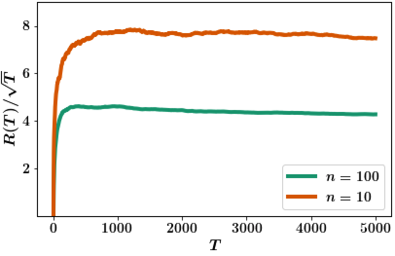
VI-A Mean-field system

Consider a complete graph $\mathcal{G}$ where the edge weights are equal to $1/n$ . Let $M$ be equal to the adjacency matrix of the graph, i.e., $M=\tfrac{1}{n}\mathds{1}_{n\times n}$ . Thus, the system dynamics are given by

x^{i}_{t+1}=Ax^{i}_{t}+Bu^{i}_{t}+D\bar{x}_{t}+E\bar{u}_{t}+w^{i}_{t},

where $\bar{x}_{t}=\tfrac{1}{n}\sum_{i\in N}x^{i}_{t}$ and $\bar{u}_{t}=\tfrac{1}{n}\sum_{i\in N}u^{i}_{t}$ . Suppose $K_{x}=K_{u}=1$ and $q_{0}=r_{0}=1/n$ and $q_{1}=r_{1}=\kappa/n$ , where $\kappa$ is a positive constant.

In this case, $M$ has rank $L=1$ , the non-zero eigenvalue of $M$ is $\lambda^{1}=1$ , the corresponding normalized eigenvector is $\tfrac{1}{\sqrt{n}}\mathds{1}_{n\times 1}$ and $q^{1}=r^{1}=q_{0}+q_{1}=(1+\kappa)/n$ . The eigenstate is given by $x^{1}_{t}=[\bar{x}_{t},\dots,\bar{x}_{t}]$ and a similar structure holds for the eigencontrol $u^{1}_{t}$ . The per-step cost can be written as (see Proposition 1)

	$\displaystyle c(x_{t},u_{t})=(1+\kappa)\bigl{[}\bar{x}_{t}^{\mathchoice{\raisebox{0.0pt}{$\displaystyle\intercal$}}{\raisebox{0.0pt}{$\textstyle\intercal$}}{\raisebox{0.0pt}{$\scriptstyle\intercal$}}{\raisebox{0.0pt}{$\scriptscriptstyle\intercal$}}}Q\bar{x}_{t}+\bar{u}_{t}^{\mathchoice{\raisebox{0.0pt}{$\displaystyle\intercal$}}{\raisebox{0.0pt}{$\textstyle\intercal$}}{\raisebox{0.0pt}{$\scriptstyle\intercal$}}{\raisebox{0.0pt}{$\scriptscriptstyle\intercal$}}}R\bar{u}_{t}\bigr{]}.$
	$\displaystyle\quad+\frac{1}{n}\sum_{i\in N}\bigl{[}(x^{i}_{t}-\bar{x}_{t})^{\mathchoice{\raisebox{0.0pt}{$\displaystyle\intercal$}}{\raisebox{0.0pt}{$\textstyle\intercal$}}{\raisebox{0.0pt}{$\scriptstyle\intercal$}}{\raisebox{0.0pt}{$\scriptscriptstyle\intercal$}}}Q(x^{i}_{t}-\bar{x}_{t})+(u^{i}_{t}-\bar{u}_{t})^{\mathchoice{\raisebox{0.0pt}{$\displaystyle\intercal$}}{\raisebox{0.0pt}{$\textstyle\intercal$}}{\raisebox{0.0pt}{$\scriptstyle\intercal$}}{\raisebox{0.0pt}{$\scriptscriptstyle\intercal$}}}R(u^{i}_{t}-\bar{u}_{t})\bigr{]}$

Thus, the system is similar to the mean-field team system investigated in [6, 7].

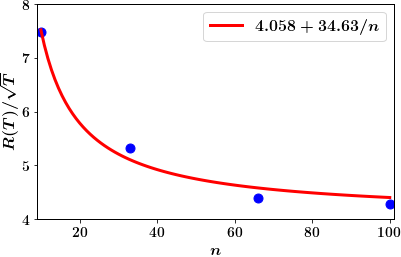
For this model, the network dependent constant $\alpha^{\mathcal{G}}$ in the regret bound of Theorem 2 is given by $\alpha^{\mathcal{G}}=\bigl{(}1+\frac{\kappa}{n}\bigr{)}=\mathcal{O}\bigl{(}1+\frac{1}{n}\bigr{)}.$ Thus, for the mean-field system, the regret of Net-TSDE scales as $\mathcal{O}(1+\tfrac{1}{n})$ with the number of agents. This is consistent with the discussion following Theorem 2.

We test these conclusions via numerical simulations of a scalar mean-field model with $d_{x}=d_{u}=1$ , $\sigma_{w}^{2}=1$ , $A=1$ , $B=0.3$ , $D=0.5$ , $E=0.2$ , $Q=1$ , $R=1$ , and $\kappa=0.5$ . The uncertain sets are chosen as $\Theta^{1}=\{\theta^{1}\in\mathds{R}^{2}:A+D+(B+E)G^{1}(\theta^{1})<\delta\}$ and $\breve{\Theta}=\{\breve{\theta}\in\mathds{R}^{2}:A+B\breve{G}(\breve{\theta})<\delta\}$ where $\delta=0.99$ . The prior over these uncertain sets is chosen according to (A6)–(A7) where $\breve{\mu}_{1}=\mu^{1}_{1}=[1,1]^{\mathchoice{\raisebox{0.0pt}{$\displaystyle\intercal$}}{\raisebox{0.0pt}{$\textstyle\intercal$}}{\raisebox{0.0pt}{$\scriptstyle\intercal$}}{\raisebox{0.0pt}{$\scriptscriptstyle\intercal$}}}$ and $\breve{\Sigma}_{1}=\Sigma^{1}_{1}=I$ . We set $T_{\min}=0$ in Net-TSDE. The system is simulated for a horizon of $T=5000$ and the expected regret $R(T)$ averaged over $500$ sample trajectories is shown in Fig. 1. As expected, the regret scales as $\tilde{\mathcal{O}}(\sqrt{T})$ with time and $\mathcal{O}\bigl{(}1+\frac{1}{n}\bigr{)}$ with the number of agents.

Refer to caption — (a) $R(T)/\sqrt{T}$ vs $T$

VI-B A general low-rank network

Figure 2: Graph

\mathcal{G}^{\circ}

with

n=4

nodes and its adjacency matrix

We consider a network with $4n$ nodes given by the graph $\mathcal{G}=\mathcal{G}^{\circ}\otimes\mathcal{C}_{n}$ , where $\mathcal{G}^{\circ}$ is a 4-node graph shown in Fig. 2 and $\mathcal{C}_{n}$ is the complete graph with $n$ nodes and each edge weight equal to $\frac{1}{n}$ . Let $M$ be the adjacency matrix of $\mathcal{G}$ which is given as $M=M^{\circ}\otimes\frac{1}{n}\mathds{1}_{n\times n}$ , where $M^{\circ}$ is the adjacency matrix of $\mathcal{G}^{\circ}$ shown in Fig. 2. Moreover, suppose $K_{x}=2$ with $q_{0}=1$ , $q_{1}=-2$ , and $q_{2}=1$ and $K_{u}=0$ with $r_{0}=1$ . Note that the cost is not normalized per-agent.

In this case, the rank of $M^{\circ}$ is $2$ with eigenvalues $\pm\rho$ , where $\rho=\sqrt{2(a^{2}+b^{2})}$ and the rank of $\frac{1}{n}\mathds{1}_{n\times n}$ is $1$ with eigenvalue $1$ . Thus, $M=M^{\circ}\otimes\frac{1}{n}\mathds{1}_{n\times n}$ has the same non-zero eigenvalues as $M^{\circ}$ given by $\lambda^{1}=\rho$ and $\lambda^{2}=-\rho$ . Further, $q^{\ell}=(1-\lambda^{\ell})^{2}$ and $r^{\ell}=1$ , for $\ell\in\{1,2\}$ . We assume that $a^{2}+b^{2}\neq 0.5$ , so that the model satisfies (A3).

For this model, the scaling parameter $\alpha^{\mathcal{G}}$ in the regret bound in Theorem 2 is given by

\alpha^{\mathcal{G}}=(1-\rho)^{2}+(1+\rho)^{2}+(4n-2)=4n+2\rho^{2}.

Recall that $\rho^{2}=(\lambda^{1})^{2}=(\lambda^{2})^{2}$ . Thus, $\alpha^{\mathcal{G}}$ has an explicit dependence on the square of the eigenvalues and the number of nodes.

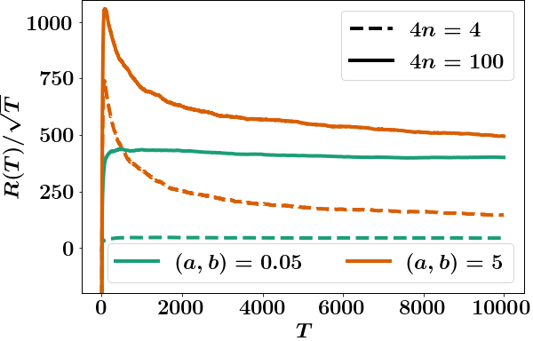
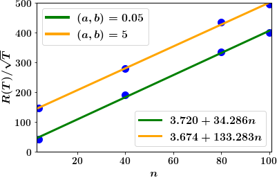
We verify this relationship via numerical simulations. We consider the graph above with two choices of parameters $(a,b)$ : (i) $a=b=0.05$ and (ii) $a=b=5$ . For both cases, we consider a scalar system with parameters same as the mean-field system considered in Sec. VI-A. The regret for both cases with different choices of number of agents $4n\in\{4,40,80,100\}$ is shown in Fig. 3. As expected, the regret scales as $\tilde{\mathcal{O}}(\sqrt{T})$ with time and $\mathcal{O}\bigl{(}4n+2\rho^{2})$ with the number of agents.

VII Conclusion

We consider the problem of controlling an unknown LQG system consisting of multiple subsystems connected over a network. By utilizing a spectral decomposition technique, we decompose the coupled subsystems into eigen and auxiliary systems. We propose a TS-based learning algorithm Net-TSDE which maintains separate posterior distributions on the unknown parameters $\theta^{\ell},\ell\in\{1,\ldots,L\}$ , and $\breve{\theta}$ associated with the eigen and auxiliary systems respectively. For each eigen-system, Net-TSDE learns the unknown parameter $\theta^{\ell}$ and controls the system in a manner similar to the TSDE algorithm for single agent LQG systems proposed in [21, 22, 41]. Consequently, the regret for each eigen system can be bounded using the results of [21, 22, 41]. However, the part of the Net-TSDE algorithm that performs learning and control for the auxiliary system has an agent selection step and thus requires additional analysis to bound its regret. Combining the regret bounds for the eigen and auxiliary systems shows that the total expected regret of Net-TSDE is upper bounded by $\tilde{\mathcal{O}}(nd_{x}^{0.5}({d_{x}+d_{u}})\sqrt{T})$ . The empirically observed scaling of regret with respect to the time horizon $T$ and the number of subsystems $n$ in our numerical experiments agrees with the theoretical upper bound.

The results presented in this paper rely on the spectral decomposition developed in [24]. A limitation of this decomposition is that the local dynamics (i.e., the $(A,B)$ matrices) are assumed to be identical for all subsystems. Interesting generalizations overcoming this limitation include settings where (i) there are multiple types of subsystems and the $(A,B)$ matrices are the same for subsystems of the same type but different across types; and (ii) the subsystems are not identical but approximately identical, i.e., there are nominal dynamics $(A^{\circ},B^{\circ})$ and the local dynamics $(A^{i},B^{i})$ of subsystem $i$ are in a small neighborhood of $(A^{\circ},B^{\circ})$ .

The decomposition in [24] exploits the fact that the dynamics and the cost couplings have the same spectrum (i.e., the same orthonormal eigenvectors). It is also possible to consider learning algorithms which exploit other features of the network such as sparsity in the case of networked MDPs [32, 33].

References

[1] N. Sandell, P. Varaiya, M. Athans, and M. Safonov, “Survey of decentralized control methods for large scale systems,” IEEE Trans. Autom. Control, vol. 23, no. 2, pp. 108–128, 1978.
[2] J. Lunze, “Dynamics of strongly coupled symmetric composite systems,” International Journal of Control, vol. 44, no. 6, pp. 1617–1640, 1986.
[3] M. K. Sundareshan and R. M. Elbanna, “Qualitative analysis and decentralized controller synthesis for a class of large-scale systems with symmetrically interconnected subsystems,” Automatica, vol. 27, no. 2, pp. 383–388, 1991.
[4] G.-H. Yang and S.-Y. Zhang, “Structural properties of large-scale systems possessing similar structures,” Automatica, vol. 31, no. 7, pp. 1011–1017, 1995.
[5] S. C. Hamilton and M. E. Broucke, “Patterned linear systems,” Automatica, vol. 48, no. 2, pp. 263–272, 2012.
[6] J. Arabneydi and A. Mahajan, “Team-optimal solution of finite number of mean-field coupled LQG subsystems,” in Conf. Decision and Control, (Kyoto, Japan), Dec. 2015.
[7] J. Arabneydi and A. Mahajan, “Linear Quadratic Mean Field Teams: Optimal and Approximately Optimal Decentralized Solutions,” 2016. arXiv:1609.00056.
[8] K. J. Astrom and B. Wittenmark, Adaptive Control. Addison-Wesley Longman Publishing Co., Inc., 1994.
[9] S. J. Bradtke, “Reinforcement learning applied to linear quadratic regulation,” in Neural Information Processing Systems, pp. 295–302, 1993.
[10] S. J. Bradtke, B. E. Ydstie, and A. G. Barto, “Adaptive linear quadratic control using policy iteration,” in Proceedings of American Control Conference, vol. 3, pp. 3475–3479, 1994.
[11] M. C. Campi and P. Kumar, “Adaptive linear quadratic Gaussian control: the cost-biased approach revisited,” SIAM Journal on Control and Optimization, vol. 36, no. 6, pp. 1890–1907, 1998.
[12] Y. Abbasi-Yadkori and C. Szepesvári, “Regret bounds for the adaptive control of linear quadratic systems,” in Annual Conference on Learning Theory, pp. 1–26, 2011.
[13] M. K. S. Faradonbeh, A. Tewari, and G. Michailidis, “Optimism-based adaptive regulation of linear-quadratic systems,” IEEE Trans. Autom. Control, vol. 66, no. 4, pp. 1802–1808, 2021.
[14] A. Cohen, T. Koren, and Y. Mansour, “Learning linear-quadratic regulators efficiently with only $\sqrt{T}$ regret,” in International Conference on Machine Learning, pp. 1300–1309, 2019.
[15] M. Abeille and A. Lazaric, “Efficient optimistic exploration in linear-quadratic regulators via Lagrangian relaxation,” in International Conference on Machine Learning, pp. 23–31, 2020.
[16] S. Dean, H. Mania, N. Matni, B. Recht, and S. Tu, “Regret bounds for robust adaptive control of the linear quadratic regulator,” in Neural Information Processing Systems, pp. 4192–4201, 2018.
[17] H. Mania, S. Tu, and B. Recht, “Certainty equivalent control of LQR is efficient.” arXiv:1902.07826, 2019.
[18] M. K. S. Faradonbeh, A. Tewari, and G. Michailidis, “Input perturbations for adaptive control and learning,” Automatica, vol. 117, p. 108950, 2020.
[19] M. Simchowitz and D. Foster, “Naive exploration is optimal for online LQR,” in International Conference on Machine Learning, pp. 8937–8948, 2020.
[20] M. K. S. Faradonbeh, A. Tewari, and G. Michailidis, “On adaptive Linear–Quadratic regulators,” Automatica, vol. 117, p. 108982, July 2020.
[21] Y. Ouyang, M. Gagrani, and R. Jain, “Control of unknown linear systems with Thompson sampling,” in Allerton Conference on Communication, Control, and Computing, pp. 1198–1205, 2017.
[22] Y. Ouyang, M. Gagrani, and R. Jain, “Posterior sampling-based reinforcement learning for control of unknown linear systems,” IEEE Trans. Autom. Control, vol. 65, no. 8, pp. 3600–3607, 2020.
[23] M. Abeille and A. Lazaric, “Improved regret bounds for Thompson sampling in linear quadratic control problems,” in International Conference on Machine Learning, pp. 1–9, 2018.
[24] S. Gao and A. Mahajan, “Optimal control of network-coupled subsystems: Spectral decomposition and low-dimensional solutions,” submitted to IEEE Trans. Control of Networked Sys., 2020.
[25] P. Auer, N. Cesa-Bianchi, and P. Fischer, “Finite-time analysis of the multiarmed bandit problem,” Machine learning, vol. 47, no. 2-3, pp. 235–256, 2002.
[26] S. Agrawal and N. Goyal, “Analysis of Thompson sampling for the multi-armed bandit problem,” in Conference on Learning Theory, 2012.
[27] H. Wang, S. Lin, H. Jafarkhani, and J. Zhang, “Distributed Q-learning with state tracking for multi-agent networked control,” in AAMAS, pp. 1692 – 1694, 2021.
[28] G. Jing, H. Bai, J. George, A. Chakrabortty, and P. K. Sharma, “Learning distributed stabilizing controllers for multi-agent systems,” IEEE Control Systems Letters, 2021.
[29] Y. Li, Y. Tang, R. Zhang, and N. Li, “Distributed reinforcement learning for decentralized linear quadratic control: A derivative-free policy optimization approach,” in Proc. Conf. Learning for Dynamics and Control, pp. 814–814, June 2020.
[30] K. Zhang, Z. Yang, H. Liu, T. Zhang, and T. Basar, “Fully decentralized multi-agent reinforcement learning with networked agents,” in International Conference on Machine Learning, pp. 5872–5881, 2018.
[31] K. Zhang, Z. Yang, and T. Başar, “Decentralized multi-agent reinforcement learning with networked agents: Recent advances,” arXiv preprint arXiv:1912.03821, 2019.
[32] I. Osband and B. Van Roy, “Near-optimal reinforcement learning in factored MDPs,” in Advances in Neural Information Processing Systems, vol. 27, Curran Associates, Inc., 2014.
[33] X. Chen, J. Hu, L. Li, and L. Wang, “Efficient reinforcement learning in factored MDPs with application to constrained RL,” arXiv preprint arXiv:2008.13319, 2021.
[34] M. Huang, P. E. Caines, and R. P. Malhamé, “Large-population cost-coupled LQG problems with nonuniform agents: individual-mass behavior and decentralized epsilon-Nash equilibria,” IEEE Transactions on Automatic Control, vol. 52, no. 9, pp. 1560–1571, 2007.
[35] J.-M. Lasry and P.-L. Lions, “Mean field games,” Japanese Journal of Mathematics, vol. 2, no. 1, pp. 229–260, 2007.
[36] J. Subramanian and A. Mahajan, “Reinforcement learning in stationary mean-field games,” in International Conference on Autonomous Agents and Multi-Agent Systems, pp. 251–259, 2019.
[37] S. G. Subramanian, P. Poupart, M. E. Taylor, and N. Hegde, “Multi type mean field reinforcement learning,” in International Conference on Autonomous Agents and Multiagent Systems, pp. 411–419, 2020.
[38] M. A. uz Zaman, K. Zhang, E. Miehling, and T. Bașar, “Reinforcement learning in non-stationary discrete-time linear-quadratic mean-field games,” in Conference on Decision and Control, pp. 2278–2284, 2020.
[39] M. Gagrani, S. Sudhakara, A. Mahajan, A. Nayyar, and Y. Ouyang, “Thompson sampling for linear quadratic mean-field teams.” arXiv preprint arXiv:2011.04686, 2020.
[40] J. Sternby, “On consistency for the method of least squares using martingale theory,” IEEE Trans. Autom. Control, vol. 22, no. 3, pp. 346–352, 1977.
[41] M. Gagrani, S. Sudhakara, A. Mahajan, A. Nayyar, and Y. Ouyang, “A relaxed technical assumption for posterior sampling-based reinforcement learning for control of unknown linear systems.” http://cim.mcgill.ca/~adityam/projects/reinforcement-learning/preprint/tsde.pdf, 2021.
[42] M. K. S. Faradonbeh, A. Tewari, and G. Michailidis, “Finite-time adaptive stabilization of linear systems,” IEEE Trans. Autom. Control, vol. 64, pp. 3498–3505, Aug. 2019.
[43] P. R. Kumar and P. Varaiya, Stochastic systems: Estimation, identification, and adaptive control. SIAM Classics, 2015.
[44] Y. Abbasi-Yadkori and C. Szepesvari, “Bayesian optimal control of smoothly parameterized systems: The lazy posterior sampling algorithm.” arXiv preprint arXiv:1406.3926, 2014.

Appendix A Appendix: Regret Analysis

A-A Preliminary Results

Since $\breve{S}(\cdot)$ and $\breve{G}(\cdot)$ are continuous functions on a compact set $\breve{\Theta}$ , there exist finite constants $\breve{M}_{J},\breve{M}_{\breve{\theta}},\breve{M}_{S},\breve{M}_{G}$ such that $\operatorname{Tr}(\breve{S}(\breve{\theta}))\leq\breve{M}_{J},\|\breve{\theta}\|\leq\breve{M}_{\breve{\theta}},\|\breve{S}(\breve{\theta})\|\leq\breve{M}_{S}$ and $\|[I,\breve{G}(\breve{\theta})^{\mathchoice{\raisebox{0.0pt}{$\displaystyle\intercal$}}{\raisebox{0.0pt}{$\textstyle\intercal$}}{\raisebox{0.0pt}{$\scriptstyle\intercal$}}{\raisebox{0.0pt}{$\scriptscriptstyle\intercal$}}}]^{\mathchoice{\raisebox{0.0pt}{$\displaystyle\intercal$}}{\raisebox{0.0pt}{$\textstyle\intercal$}}{\raisebox{0.0pt}{$\scriptstyle\intercal$}}{\raisebox{0.0pt}{$\scriptscriptstyle\intercal$}}}\|\leq\breve{M}_{G}$ for all $\breve{\theta}\in\breve{\Theta}$ where $\|\cdot\|$ is the induced matrix norm.

Let $\breve{X}^{i}_{T}=\max_{1\leq t\leq T}\|\breve{x}^{i}_{t}\|$ be the maximum norm of the auxiliary state along the entire trajectory. The next bound follows from [41, Lemma 4].

Lemma 4

For each node $i\in N$ , any $q\geq 1$ and any $T>1$ ,

\displaystyle\mathbb{E}\biggl{[}\frac{(\breve{X}_{T}^{i})^{q}}{(\breve{\sigma}^{i})^{q}}\biggr{]}

\displaystyle\leq\mathcal{O}\big{(}\log T\big{)}

_□

The following lemma gives an upper bound on the number of episodes $\breve{K}_{T}$ .

Lemma 5

For any $q\geq 1$ , we have

	$\displaystyle\mathbb{E}\biggl{[}\frac{(\breve{X}_{T}^{i})^{q}}{(\breve{\sigma}^{i})^{q}}\log\biggl{(}\sum_{t=1}^{T}(\breve{X}_{T}^{j_{t}})^{2}\biggr{)}\biggr{]}$	$\displaystyle\leq\mathbb{E}\biggl{[}\frac{(\breve{X}_{T}^{i})^{q}}{(\breve{\sigma}^{i})^{q}}\log\biggl{(}\sum_{t=1}^{T}\sum_{i\in N}(\breve{X}_{T}^{i})^{2}\biggr{)}\biggr{]}$
		$\displaystyle\leq\tilde{\mathcal{O}}(1)$		(39)

_□

This can be proved along the same lines as [41, Lemma 5].

Lemma 6

The number of episodes $\breve{K}_{T}$ is bounded as follows:

\displaystyle\breve{K}_{T}

\displaystyle\leq\mathcal{O}\left(\sqrt{(d_{x}+d_{u})T\log\left(\sum_{t=1}^{T-1}\frac{(\breve{X}_{T}^{j_{t}})^{2}}{(\breve{\sigma}^{j_{t}})^{2}}\right)}\right)

_□

Proof

We can follow the same argument as in the proof of Lemma 5 in [41]. Let $\breve{\eta}-1$ be the number of times the second stopping criterion is triggered for $\breve{p}_{t}$ . Using the analysis in the proof of Lemma 5 in [41], we can get the following inequalities:

	$\displaystyle\breve{K}_{T}$	$\displaystyle\leq\sqrt{2\breve{\eta}T},$		(40)
	$\displaystyle\det(\breve{\Sigma}^{-1}_{T})$	$\displaystyle\geq 2^{\breve{\eta}-1}\det(\breve{\Sigma}^{-1}_{1})\geq 2^{\breve{\eta}-1}\breve{\lambda}_{\min}^{d},$		(41)

where $d=d_{x}+d_{u}$ and $\breve{\lambda}_{\min}$ is the minimum eigenvalue of $\breve{\Sigma}_{1}^{-1}$ .

Combining (41) with $\operatorname{Tr}(\breve{\Sigma}_{T}^{-1})/d\geq\det(\breve{\Sigma}_{T}^{-1})^{1/d}$ , we get $\operatorname{Tr}(\breve{\Sigma}_{T}^{-1})\geq d\breve{\lambda}_{\min}2^{(\breve{\eta}-1)/d}.$ Thus,

\eta\leq 1+\frac{d}{\log 2}\log\biggl{(}\frac{\operatorname{Tr}(\breve{\Sigma}_{T}^{-1})}{d\breve{\lambda}_{\min}}\biggr{)}.

(42)

Now, we bound $\operatorname{Tr}(\breve{\Sigma}_{T}^{-1})$ . From (29b), we have

\operatorname{Tr}(\breve{\Sigma}_{T}^{-1})=\operatorname{Tr}(\breve{\Sigma}_{1}^{-1})+\sum_{t=1}^{T-1}\frac{1}{(\breve{\sigma}^{j_{t}})^{2}}\underbrace{\operatorname{Tr}(\breve{z}_{t}^{j_{t}}(\breve{z}_{t}^{j_{t}})^{\mathchoice{\raisebox{0.0pt}{$\displaystyle\intercal$}}{\raisebox{0.0pt}{$\textstyle\intercal$}}{\raisebox{0.0pt}{$\scriptstyle\intercal$}}{\raisebox{0.0pt}{$\scriptscriptstyle\intercal$}}}}_{=\|\breve{z}_{t}^{j_{t}}\|^{2}}).

(43)

Note that $\|\breve{z}_{t}^{j_{t}}\|=\|[I,\breve{G}(\breve{\theta})^{\mathchoice{\raisebox{0.0pt}{$\displaystyle\intercal$}}{\raisebox{0.0pt}{$\textstyle\intercal$}}{\raisebox{0.0pt}{$\scriptstyle\intercal$}}{\raisebox{0.0pt}{$\scriptscriptstyle\intercal$}}}]^{\mathchoice{\raisebox{0.0pt}{$\displaystyle\intercal$}}{\raisebox{0.0pt}{$\textstyle\intercal$}}{\raisebox{0.0pt}{$\scriptstyle\intercal$}}{\raisebox{0.0pt}{$\scriptscriptstyle\intercal$}}}\breve{x}_{t}^{j_{t}}\|\leq\breve{M}_{G}\|\breve{x}_{t}^{j_{t}}\|\leq\breve{M}_{G}\breve{X}_{T}^{j_{t}}$ . Using $\|\breve{z}_{t}^{j_{t}}\|^{2}\leq\breve{M}_{G}^{2}(\breve{X}_{T}^{j_{t}})^{2}$ in (43) and substituting the resulting bound on $\operatorname{Tr}(\breve{\Sigma}_{T}^{-1})$ in (42) and then combining it with the bound on $\eta$ in (40), gives the result of the lemma. _■

Lemma 7

The expected value of $\breve{K}_{T}$ is bounded as follows:

\displaystyle\mathbb{E}[\breve{K}_{T}]

\displaystyle\leq\tilde{\mathcal{O}}\left(\sqrt{(d_{x}+d_{u})T}\right)

_□

Proof

From Lemma 6, we get

	$\displaystyle\mathbb{E}[\breve{K}_{T}]$	$\displaystyle\leq\mathcal{O}\Biggl{(}\mathbb{E}\Biggl{[}\sqrt{(d_{x}+d_{u})T\log\biggl{(}\sum_{t=1}^{T-1}\frac{(\breve{X}_{T}^{j_{t}})^{2}}{(\breve{\sigma}^{j_{t}})^{2}}\biggr{)}}\Biggr{]}\Biggr{)}$
		$\displaystyle\stackrel{{\scriptstyle(a)}}{{\leq}}\mathcal{O}\biggl{(}\sqrt{(d_{x}+d_{u})T\log\biggl{(}\mathbb{E}\biggl{[}\sum_{t=1}^{T-1}\frac{(\breve{X}_{T}^{j_{t}})^{2}}{(\breve{\sigma}^{j_{t}})^{2}}\biggr{]}\biggr{)}}\biggr{)}$
		$\displaystyle\leq\mathcal{O}\biggl{(}\sqrt{(d_{x}+d_{u})T\log\biggl{(}\mathbb{E}\biggl{[}\sum_{t=1}^{T-1}\sum_{i\in N}\frac{(\breve{X}_{T}^{i})^{2}}{(\breve{\sigma}^{i})^{2}}\biggr{]}\biggr{)}}\biggr{)}$
		$\displaystyle\stackrel{{\scriptstyle(b)}}{{\leq}}\tilde{\mathcal{O}}(\sqrt{(d_{x}+d_{u})T})$

where $(a)$ follows from Jensen’s inequality and $(b)$ follows from Lemma 4. _■

A-B Proof of Lemma 3

Proof

We will prove each part separately.

1) Bounding $\breve{R}^{i}_{0}(T)$ : From an argument similar to the proof of Lemma 5 of [22], we get that $\breve{R}^{i}_{0}(T)\leq(\breve{\sigma}^{i})^{2}\breve{M}_{J}\mathbb{E}[\breve{K}_{T}].$ The result then follows from substituting the bound on $\mathbb{E}[\breve{K}_{T}]$ from Lemma 7.

2) Bounding $\breve{R}^{i}_{1}(T)$ :

$\displaystyle\breve{R}^{i}_{1}(T)$	$\displaystyle=\mathbb{E}\biggl{[}\sum_{k=1}^{\breve{K}_{T}}\sum_{t=\breve{t}_{k}}^{\breve{t}_{k+1}-1}\Big{[}(\breve{x}_{t}^{i})^{\mathchoice{\raisebox{0.0pt}{$\displaystyle\intercal$}}{\raisebox{0.0pt}{$\textstyle\intercal$}}{\raisebox{0.0pt}{$\scriptstyle\intercal$}}{\raisebox{0.0pt}{$\scriptscriptstyle\intercal$}}}\breve{S}_{k}\breve{x}_{t}^{i}-(\breve{x}_{t+1}^{i})^{\mathchoice{\raisebox{0.0pt}{$\displaystyle\intercal$}}{\raisebox{0.0pt}{$\textstyle\intercal$}}{\raisebox{0.0pt}{$\scriptstyle\intercal$}}{\raisebox{0.0pt}{$\scriptscriptstyle\intercal$}}}\breve{S}_{k}\breve{x}_{t+1}^{i}\Big{]}\biggr{]}$
	$\displaystyle=\mathbb{E}\biggl{[}\sum_{k=1}^{\breve{K}_{T}}\Big{[}(\breve{x}^{i}_{\breve{t}_{k}})^{\mathchoice{\raisebox{0.0pt}{$\displaystyle\intercal$}}{\raisebox{0.0pt}{$\textstyle\intercal$}}{\raisebox{0.0pt}{$\scriptstyle\intercal$}}{\raisebox{0.0pt}{$\scriptscriptstyle\intercal$}}}\breve{S}_{k}\breve{x}_{\breve{t}_{k}}^{i}-(\breve{x}_{\breve{t}_{k+1}}^{i})^{\mathchoice{\raisebox{0.0pt}{$\displaystyle\intercal$}}{\raisebox{0.0pt}{$\textstyle\intercal$}}{\raisebox{0.0pt}{$\scriptstyle\intercal$}}{\raisebox{0.0pt}{$\scriptscriptstyle\intercal$}}}\breve{S}_{k}\breve{x}_{\breve{t}_{k+1}}^{i}\Big{]}\biggr{]}$
	$\displaystyle\leq\mathbb{E}\biggl{[}\sum_{k=1}^{\breve{K}_{T}}(\breve{x}^{i}_{\breve{t}_{k}})^{\mathchoice{\raisebox{0.0pt}{$\displaystyle\intercal$}}{\raisebox{0.0pt}{$\textstyle\intercal$}}{\raisebox{0.0pt}{$\scriptstyle\intercal$}}{\raisebox{0.0pt}{$\scriptscriptstyle\intercal$}}}\breve{S}_{k}\breve{x}_{\breve{t}_{k}}^{i}\biggr{]}\leq\mathbb{E}\biggl{[}\sum_{k=1}^{\breve{K}_{T}}\\|\breve{S}_{k}\\|\\|\breve{x}_{t_{k}}^{i}\\|^{2}\biggr{]}$
	$\displaystyle\leq\breve{M}_{S}\mathbb{E}[\breve{K}_{T}(\breve{X}_{T}^{i})^{2}]$	(44)

where the last inequality follows from $\|\breve{S}_{k}\|\leq\breve{M}_{S}$ . Using the bound for $\breve{K}_{T}$ in Lemma 6, we get

\breve{R}^{i}_{1}(T)\leq\mathcal{O}\Biggl{(}\sqrt{(d_{x}+d_{u})T}\,\mathbb{E}\Biggl{[}(\breve{X}^{i}_{T})^{2}\sqrt{\log\biggl{(}\sum_{t=1}^{T-1}\frac{(\breve{X}_{T}^{j_{t}})^{2}}{(\breve{\sigma}^{j_{t}})^{2}}\biggr{)}}\Biggr{]}\Biggr{)}.

(45)

Now, consider the term

		$\displaystyle\hskip-10.00002pt\mathbb{E}\Biggl{[}(\breve{X}^{i}_{T})^{2}\sqrt{\log\biggl{(}\sum_{t=1}^{T-1}\frac{(\breve{X}_{T}^{j_{t}})^{2}}{(\breve{\sigma}^{j_{t}})^{2}}\biggr{)}}\Biggr{]}\Biggr{)}$
		$\displaystyle\stackrel{{\scriptstyle(a)}}{{\leq}}\sqrt{\mathbb{E}[(\breve{X}^{i}_{T})^{4}]\;\mathbb{E}\biggl{[}\log\biggl{(}\sum_{t=1}^{T-1}\frac{(\breve{X}_{T}^{j_{t}})^{2}}{(\breve{\sigma}^{j_{t}})^{2}}\biggr{)}\biggr{]}}$
		$\displaystyle\stackrel{{\scriptstyle(b)}}{{\leq}}\sqrt{\mathbb{E}[(\breve{X}^{i}_{T})^{4}]\;\log\biggl{(}\mathbb{E}\biggl{[}\sum_{t=1}^{T-1}\sum_{i\in N}\frac{(\breve{X}_{T}^{i})^{2}}{(\breve{\sigma}^{j_{t}})^{2}}\biggr{]}\biggr{)}}$
		$\displaystyle\stackrel{{\scriptstyle(c)}}{{\leq}}\tilde{\mathcal{O}}((\breve{\sigma}^{i})^{2}),$		(46)

where $(a)$ follows from Cauchy-Schwarz, $(b)$ follows from Jensen’s inequality and $(c)$ follows from Lemma 4. The result then follows from substituting (46) in (44).

3) Bounding $\breve{R}^{i}_{2}(T)$ : As in [22], we can bound the inner summand in $\breve{R}^{i}_{2}(T)$ as

\bigl{[}(\breve{\theta}^{\mathchoice{\raisebox{0.0pt}{$\displaystyle\intercal$}}{\raisebox{0.0pt}{$\textstyle\intercal$}}{\raisebox{0.0pt}{$\scriptstyle\intercal$}}{\raisebox{0.0pt}{$\scriptscriptstyle\intercal$}}}\breve{z}^{i}_{t})^{\mathchoice{\raisebox{0.0pt}{$\displaystyle\intercal$}}{\raisebox{0.0pt}{$\textstyle\intercal$}}{\raisebox{0.0pt}{$\scriptstyle\intercal$}}{\raisebox{0.0pt}{$\scriptscriptstyle\intercal$}}}\breve{{S}}_{k}(\breve{\theta}^{\mathchoice{\raisebox{0.0pt}{$\displaystyle\intercal$}}{\raisebox{0.0pt}{$\textstyle\intercal$}}{\raisebox{0.0pt}{$\scriptstyle\intercal$}}{\raisebox{0.0pt}{$\scriptscriptstyle\intercal$}}}\breve{z}^{i}_{t})-(\breve{\theta}_{k}^{\mathchoice{\raisebox{0.0pt}{$\displaystyle\intercal$}}{\raisebox{0.0pt}{$\textstyle\intercal$}}{\raisebox{0.0pt}{$\scriptstyle\intercal$}}{\raisebox{0.0pt}{$\scriptscriptstyle\intercal$}}}\breve{z}^{i}_{t})^{\mathchoice{\raisebox{0.0pt}{$\displaystyle\intercal$}}{\raisebox{0.0pt}{$\textstyle\intercal$}}{\raisebox{0.0pt}{$\scriptstyle\intercal$}}{\raisebox{0.0pt}{$\scriptscriptstyle\intercal$}}}\breve{{S}}_{k}((\breve{\theta}_{k})^{\mathchoice{\raisebox{0.0pt}{$\displaystyle\intercal$}}{\raisebox{0.0pt}{$\textstyle\intercal$}}{\raisebox{0.0pt}{$\scriptstyle\intercal$}}{\raisebox{0.0pt}{$\scriptscriptstyle\intercal$}}}\breve{z}^{i}_{t})\bigr{]}\\ \leq\mathcal{O}(\breve{X}_{T}^{i}\|(\breve{\theta}-\breve{\theta}_{k})^{\mathchoice{\raisebox{0.0pt}{$\displaystyle\intercal$}}{\raisebox{0.0pt}{$\textstyle\intercal$}}{\raisebox{0.0pt}{$\scriptstyle\intercal$}}{\raisebox{0.0pt}{$\scriptscriptstyle\intercal$}}}\breve{z}_{t}^{i}\|).

Therefore,

\breve{R}^{i}_{2}(T)\leq\mathcal{O}\biggl{(}\mathbb{E}\Big{[}\breve{X}_{T}^{i}\sum_{k=1}^{\breve{K}_{T}}\sum_{t=\breve{t}_{k}}^{\breve{t}_{k+1}-1}\|(\breve{\theta}-\breve{\theta}_{k})^{\mathchoice{\raisebox{0.0pt}{$\displaystyle\intercal$}}{\raisebox{0.0pt}{$\textstyle\intercal$}}{\raisebox{0.0pt}{$\scriptstyle\intercal$}}{\raisebox{0.0pt}{$\scriptscriptstyle\intercal$}}}\breve{z}_{t}^{i}\|\Big{]}\biggr{)}.

(47)

The term inside $\mathcal{O}(\cdot)$ can be written as

	$\displaystyle\mathbb{E}\bigg{[}\breve{X}_{T}^{i}\sum_{k=1}^{\breve{K}_{T}}\sum_{t=\breve{t}_{k}}^{\breve{t}_{k+1}-1}\\|(\breve{\theta}-\breve{\theta}_{k})^{\mathchoice{\raisebox{0.0pt}{$\displaystyle\intercal$}}{\raisebox{0.0pt}{$\textstyle\intercal$}}{\raisebox{0.0pt}{$\scriptstyle\intercal$}}{\raisebox{0.0pt}{$\scriptscriptstyle\intercal$}}}\breve{z}_{t}^{i}\\|\bigg{]}$
	$\displaystyle\quad=\mathbb{E}\bigg{[}\breve{X}_{T}^{i}\sum_{k=1}^{\breve{K}_{T}}\sum_{t=\breve{t}_{k}}^{\breve{t}_{k+1}-1}\\|(\breve{\Sigma}^{-0.5}_{{\color[rgb]{0,0,0}\definecolor[named]{pgfstrokecolor}{rgb}{0,0,0}\pgfsys@color@gray@stroke{0}\pgfsys@color@gray@fill{0}t_{k}}}(\breve{\theta}-\breve{\theta}_{k}))^{\mathchoice{\raisebox{0.0pt}{$\displaystyle\intercal$}}{\raisebox{0.0pt}{$\textstyle\intercal$}}{\raisebox{0.0pt}{$\scriptstyle\intercal$}}{\raisebox{0.0pt}{$\scriptscriptstyle\intercal$}}}\breve{\Sigma}^{0.5}_{{\color[rgb]{0,0,0}\definecolor[named]{pgfstrokecolor}{rgb}{0,0,0}\pgfsys@color@gray@stroke{0}\pgfsys@color@gray@fill{0}t_{k}}}\breve{z}_{t}^{i}\\|\bigg{]}$
	$\displaystyle\quad\leq\mathbb{E}\bigg{[}\sum_{k=1}^{\breve{K}_{T}}\sum_{t=\breve{t}_{k}}^{\breve{t}_{k+1}-1}\\|\breve{\Sigma}^{-0.5}_{{\color[rgb]{0,0,0}\definecolor[named]{pgfstrokecolor}{rgb}{0,0,0}\pgfsys@color@gray@stroke{0}\pgfsys@color@gray@fill{0}t_{k}}}(\breve{\theta}-\breve{\theta}_{k})\\|\times\breve{X}_{T}^{i}\\|\breve{\Sigma}^{0.5}_{{\color[rgb]{0,0,0}\definecolor[named]{pgfstrokecolor}{rgb}{0,0,0}\pgfsys@color@gray@stroke{0}\pgfsys@color@gray@fill{0}t_{k}}}\breve{z}_{t}^{i}\\|\bigg{]}$
	$\displaystyle\quad\leq\sqrt{\mathbb{E}\bigg{[}\sum_{k=1}^{\breve{K}_{T}}\sum_{t=\breve{t}_{k}}^{\breve{t}_{k+1}-1}\\|\breve{\Sigma}^{-0.5}_{{\color[rgb]{0,0,0}\definecolor[named]{pgfstrokecolor}{rgb}{0,0,0}\pgfsys@color@gray@stroke{0}\pgfsys@color@gray@fill{0}t_{k}}}(\breve{\theta}-\breve{\theta}_{k})\\|^{2}\bigg{]}}$
	$\displaystyle\qquad\times\sqrt{\mathbb{E}\bigg{[}\sum_{k=1}^{\breve{K}_{T}}\sum_{t=\breve{t}_{k}}^{\breve{t}_{k+1}-1}(\breve{X}_{T}^{i})^{2}\\|\breve{\Sigma}^{0.5}_{{\color[rgb]{0,0,0}\definecolor[named]{pgfstrokecolor}{rgb}{0,0,0}\pgfsys@color@gray@stroke{0}\pgfsys@color@gray@fill{0}t_{k}}}\breve{z}_{t}^{i}\\|^{2}\bigg{]}}$		(48)

where the last inequality follows from Cauchy-Schwarz inequality.

Following the same argument as [41, Lemma 7], the first part of (48) is bounded by

\mathbb{E}\bigg{[}\sum_{k=1}^{\breve{K}_{T}}\sum_{t=\breve{t}_{k}}^{\breve{t}_{k+1}-1}\|\breve{\Sigma}^{-0.5}_{{\color[rgb]{0,0,0}\definecolor[named]{pgfstrokecolor}{rgb}{0,0,0}\pgfsys@color@gray@stroke{0}\pgfsys@color@gray@fill{0}t_{k}}}(\breve{\theta}-\breve{\theta}_{k})\|^{2}\bigg{]}\leq\mathcal{O}(d_{x}(d_{x}+d_{u})T).

(49)

For the second part of the bound in (48), we follow the same argument as [41, Lemma 8]. Recall that $\breve{\lambda}_{\min}$ is the smallest eigenvalue of $\breve{\Sigma}_{1}^{-1}$ . Therefore, by (29b), all eigenvalues of $\breve{\Sigma}_{t}^{-1}$ are no smaller than $\breve{\lambda}_{\min}$ . Or, equivalently, all eigenvalues of $\breve{\Sigma}_{t}$ are no larger than $1/\breve{\lambda}_{\min}$ .

Using [12, Lemma 11], we can show that for any $t\in\{t_{k},\dots,t_{k+1}-1\}$ ,

	$\displaystyle\\|\breve{\Sigma}^{0.5}_{t_{k}}\breve{z}_{t}^{i}\\|^{2}$	$\displaystyle=(\breve{z}^{i}_{t})^{\mathchoice{\raisebox{0.0pt}{$\displaystyle\intercal$}}{\raisebox{0.0pt}{$\textstyle\intercal$}}{\raisebox{0.0pt}{$\scriptstyle\intercal$}}{\raisebox{0.0pt}{$\scriptscriptstyle\intercal$}}}\breve{\Sigma}_{t_{k}}\breve{z}^{i}_{t}\leq\frac{\det\breve{\Sigma}_{t}^{-1}}{\det\breve{\Sigma}_{t_{k}}^{-1}}(\breve{z}^{i}_{t})^{\mathchoice{\raisebox{0.0pt}{$\displaystyle\intercal$}}{\raisebox{0.0pt}{$\textstyle\intercal$}}{\raisebox{0.0pt}{$\scriptstyle\intercal$}}{\raisebox{0.0pt}{$\scriptscriptstyle\intercal$}}}\breve{\Sigma}_{t}\breve{z}^{i}_{t}$
		$\displaystyle\leq F_{1}(\breve{X}^{i}_{T})\,(\breve{z}^{i}_{t})^{\mathchoice{\raisebox{0.0pt}{$\displaystyle\intercal$}}{\raisebox{0.0pt}{$\textstyle\intercal$}}{\raisebox{0.0pt}{$\scriptstyle\intercal$}}{\raisebox{0.0pt}{$\scriptscriptstyle\intercal$}}}\breve{\Sigma}_{t}\breve{z}^{i}_{t}$		(50)

where $F_{1}(\breve{X}^{i}_{T})=\bigl{(}1+(\breve{M}_{G}^{2}(\breve{X}^{i}_{T})^{2}/{\breve{\lambda}_{\min}\breve{\sigma}_{w}^{2}})\bigr{)}^{\breve{T}_{\min}\vee 1}$ and the last inequality follows from [41, Lemma 10].

Moreover, since all eigenvalues of $\breve{\Sigma}_{t}$ are no larger than $1/\breve{\lambda}_{\min}$ , we have $(\breve{z}^{i}_{t})^{\mathchoice{\raisebox{0.0pt}{$\displaystyle\intercal$}}{\raisebox{0.0pt}{$\textstyle\intercal$}}{\raisebox{0.0pt}{$\scriptstyle\intercal$}}{\raisebox{0.0pt}{$\scriptscriptstyle\intercal$}}}\breve{\Sigma}_{t}\breve{z}^{i}_{t}\leq\|\breve{z}^{i}_{t}\|^{2}/{\breve{\lambda}_{\min}}\leq\breve{M}_{G}^{2}(\breve{X}^{i}_{T})^{2}/{\breve{\lambda}_{\min}}$ . Therefore,

		$\displaystyle\hskip-20.00003pt(\breve{z}^{i}_{t})^{\mathchoice{\raisebox{0.0pt}{$\displaystyle\intercal$}}{\raisebox{0.0pt}{$\textstyle\intercal$}}{\raisebox{0.0pt}{$\scriptstyle\intercal$}}{\raisebox{0.0pt}{$\scriptscriptstyle\intercal$}}}\breve{\Sigma}_{t}\breve{z}^{i}_{t}\leq\biggl{(}(\breve{\sigma}^{i})^{2}\vee\frac{\breve{M}_{G}^{2}(\breve{X}^{i}_{T})^{2}}{\breve{\lambda}_{\min}}\biggr{)}\biggl{(}1\wedge\frac{(\breve{z}^{i}_{t})^{\mathchoice{\raisebox{0.0pt}{$\displaystyle\intercal$}}{\raisebox{0.0pt}{$\textstyle\intercal$}}{\raisebox{0.0pt}{$\scriptstyle\intercal$}}{\raisebox{0.0pt}{$\scriptscriptstyle\intercal$}}}\breve{\Sigma}_{t}\breve{z}^{i}_{t}}{(\breve{\sigma}^{i})^{2}}\biggr{)}$
		$\displaystyle\leq\biggl{(}(\breve{\sigma}^{i})^{2}+\frac{\breve{M}_{G}^{2}(\breve{X}^{i}_{T})^{2}}{\breve{\lambda}_{\min}}\biggr{)}\biggl{(}1\wedge\frac{(\breve{z}^{j_{t}}_{t})^{\mathchoice{\raisebox{0.0pt}{$\displaystyle\intercal$}}{\raisebox{0.0pt}{$\textstyle\intercal$}}{\raisebox{0.0pt}{$\scriptstyle\intercal$}}{\raisebox{0.0pt}{$\scriptscriptstyle\intercal$}}}\breve{\Sigma}_{t}\breve{z}^{j_{t}}_{t}}{(\breve{\sigma}^{j_{t}})^{2}}\biggr{)},$		(51)

where the last inequality follows from the definition of $j_{t}$ . Let $F_{2}(\breve{X}^{i}_{T})=\bigl{(}(\breve{\sigma}^{i})^{2}+({\breve{\lambda}_{\min}}/{\breve{M}_{G}^{2}(\breve{X}^{i}_{T})^{2}})\bigr{)}$ . Then,

		$\displaystyle\hskip-10.00002pt\sum_{t=1}^{T}(\breve{z}^{i}_{t})^{\mathchoice{\raisebox{0.0pt}{$\displaystyle\intercal$}}{\raisebox{0.0pt}{$\textstyle\intercal$}}{\raisebox{0.0pt}{$\scriptstyle\intercal$}}{\raisebox{0.0pt}{$\scriptscriptstyle\intercal$}}}\breve{\Sigma}_{t}\breve{z}^{i}_{t}\leq F_{2}(\breve{X}^{i}_{T})\sum_{t=1}^{T}\biggl{(}1\wedge\frac{(\breve{z}^{j_{t}}_{t})^{\mathchoice{\raisebox{0.0pt}{$\displaystyle\intercal$}}{\raisebox{0.0pt}{$\textstyle\intercal$}}{\raisebox{0.0pt}{$\scriptstyle\intercal$}}{\raisebox{0.0pt}{$\scriptscriptstyle\intercal$}}}\breve{\Sigma}_{t}\breve{z}^{j_{t}}_{t}}{(\breve{\sigma}^{j_{t}})^{2}}\biggr{)}$
		$\displaystyle=F_{2}(\breve{X}^{i}_{T})\sum_{t=1}^{T}\biggl{(}1\wedge\biggl{\lVert}\frac{\Sigma^{0.5}_{t}\breve{z}^{j_{t}}_{t}(\breve{z}^{j_{t}}_{t})^{\mathchoice{\raisebox{0.0pt}{$\displaystyle\intercal$}}{\raisebox{0.0pt}{$\textstyle\intercal$}}{\raisebox{0.0pt}{$\scriptstyle\intercal$}}{\raisebox{0.0pt}{$\scriptscriptstyle\intercal$}}}\Sigma^{0.5}_{t}}{(\breve{\sigma}^{j_{t}})^{2}}\biggr{\rVert}\biggr{)}$
		$\displaystyle\stackrel{{\scriptstyle(a)}}{{\leq}}F_{2}(\breve{X}^{i}_{T})\biggl{[}2d\log\bigg{(}\frac{\operatorname{Tr}(\breve{\Sigma}_{T+1}^{-1})}{d}\biggr{)}-\log\det\Sigma^{-1}_{1}\biggr{]}$
		$\displaystyle\stackrel{{\scriptstyle(b)}}{{\leq}}F_{2}(\breve{X}^{i}_{T})\biggl{[}2d\log\biggl{(}\frac{1}{d}\biggl{(}\operatorname{Tr}(\breve{\Sigma}_{1}^{-1})+\breve{M}_{G}\sum_{t=1}^{T}\frac{(\breve{X}^{j_{t}}_{T})^{2}}{(\breve{\sigma}^{j_{t}})^{2}}\biggr{)}\biggr{)}$
		$\displaystyle\hskip 60.00009pt-\log\det\Sigma^{-1}_{1}\biggr{]}$		(52)

where $d=d_{x}+d_{u}$ and $(a)$ follows from (29b) and the intermediate step in the proof of [44, Lemma 6]. and $(b)$ follows from (43) and the subsequent discussion.

Using (50) and (52), we can bound the second term of (48) as follows

	$\displaystyle\mathbb{E}\Big{[}\sum_{t=1}^{T}(\breve{X}_{T}^{i})^{2}\\|\breve{\Sigma}^{0.5}_{t_{k}}\breve{z}_{t}^{i}\\|^{2}\Big{]}\leq\mathcal{O}\biggl{(}d\,\mathbb{E}\biggl{[}F_{1}(\breve{X}^{i}_{t})F_{2}(\breve{X}^{i}_{T})(\breve{X}^{i}_{T})^{2}$
	$\displaystyle\hskip 120.00018pt\times\log\biggl{(}\sum_{t=1}^{T}(\breve{X}_{T}^{j_{t}})^{2}\biggr{)}\biggr{]}\biggr{)}$
	$\displaystyle\leq\mathcal{O}\biggl{(}d(\breve{\sigma}^{i})^{4}\mathbb{E}\biggl{[}F_{1}(\breve{X}^{i}_{T})\frac{F_{2}(\breve{X}^{i}_{T})}{(\breve{\sigma}^{i})^{2}}\frac{(\breve{X}^{i}_{T})^{2}}{(\breve{\sigma}^{i})^{2}}\log\biggl{(}\sum_{t=1}^{T}(\breve{X}_{T}^{j_{t}})^{2}\biggr{)}\biggr{]}\biggr{)}$
	$\displaystyle\leq\tilde{\mathcal{O}}(d(\breve{\sigma}^{i})^{4})$		(53)

where the last inequality follows by observing that $F_{1}(\breve{X}^{i}_{T})\frac{F_{2}(\breve{X}^{i}_{T})}{(\breve{\sigma}^{i})^{2}}\frac{(\breve{X}^{i}_{T})^{2}}{(\breve{\sigma}^{i})^{2}}\log\bigl{(}\sum_{t=1}^{T}(\breve{X}_{T}^{j_{t}})^{2}\bigr{)}$ is a polynomial in $\breve{X}^{i}_{T}/\breve{\sigma}^{i}$ multiplied by $\log(\sum_{t=1}^{T}(X^{j_{i}}_{T})^{2})$ and, using Lemma 5.

The result then follows by substituting (49) and (53) in (48).

_■

Sagar Sudhakara received M.Tech Degree in the area of Communication and Signal Processing from Indian Institute of Technology Bombay, Mumbai, India, in 2016 and is currently pursuing PhD in Electrical and Computer Engineering at University of Southern California. He is a recipient of USC Annenberg fellowship and his research interests include reinforcement learning and decentralized stochastic control.

Aditya Mahajan (S’06-M’09-SM’14) is Associate Professor in the the department of Electrical and Computer Engineering, McGill University, Montreal, Canada. He currently serves as Associate Editor of Mathematics of Control, Signal, and Systems. He is the recipient of the 2015 George Axelby Outstanding Paper Award, 2014 CDC Best Student Paper Award (as supervisor), and the 2016 NecSys Best Student Paper Award (as supervisor). His principal research interests include learning and control of centralized and decentralized stochastic systems.

Ashutosh Nayyar (S’09-M’11-SM’18) received the B.Tech. degree in electrical engineering from the Indian Institute of Technology, Delhi, India, in 2006. He received the M.S. degree in electrical engineering and computer science in 2008, the MS degree in applied mathematics in 2011, and the Ph.D. degree in electrical engineering and computer science in 2011, all from the University of Michigan, Ann Arbor. He was a Post-Doctoral Researcher at the University of Illinois at Urbana-Champaign and at the University of California, Berkeley before joining the University of Southern California in 2014. His research interests are in decentralized stochastic control, decentralized decision-making in sensing and communication systems, reinforcement learning, game theory, mechanism design and electric energy systems.

Yi Ouyang received the B.S. degree in Electrical Engineering from the National Taiwan University, Taipei, Taiwan in 2009, and the M.Sc and Ph.D. in Electrical Engineering and Computer Science at the University of Michigan, in 2012 and 2015, respectively. He is currently a researcher at Preferred Networks, Burlingame, CA. His research interests include reinforcement learning, stochastic control, and stochastic dynamic games.

	$\displaystyle\mathbb{E}\bigg{[}\breve{X}_{T}^{i}\sum_{k=1}^{\breve{K}_{T}}\sum_{t=\breve{t}_{k}}^{\breve{t}_{k+1}-1}\\|(\breve{\theta}-\breve{\theta}_{k})^{\mathchoice{\raisebox{0.0pt}{$\displaystyle\intercal$}}{\raisebox{0.0pt}{$\textstyle\intercal$}}{\raisebox{0.0pt}{$\scriptstyle\intercal$}}{\raisebox{0.0pt}{$\scriptscriptstyle\intercal$}}}\breve{z}_{t}^{i}\\|\bigg{]}$
	$\displaystyle\quad=\mathbb{E}\bigg{[}\breve{X}_{T}^{i}\sum_{k=1}^{\breve{K}_{T}}\sum_{t=\breve{t}_{k}}^{\breve{t}_{k+1}-1}\\|(\breve{\Sigma}^{-0.5}_{{\color[rgb]{0,0,0}\definecolor[named]{pgfstrokecolor}{rgb}{0,0,0}\pgfsys@color@gray@stroke{0}\pgfsys@color@gray@fill{0}t_{k}}}(\breve{\theta}-\breve{\theta}_{k}))^{\mathchoice{\raisebox{0.0pt}{$\displaystyle\intercal$}}{\raisebox{0.0pt}{$\textstyle\intercal$}}{\raisebox{0.0pt}{$\scriptstyle\intercal$}}{\raisebox{0.0pt}{$\scriptscriptstyle\intercal$}}}\breve{\Sigma}^{0.5}_{{\color[rgb]{0,0,0}\definecolor[named]{pgfstrokecolor}{rgb}{0,0,0}\pgfsys@color@gray@stroke{0}\pgfsys@color@gray@fill{0}t_{k}}}\breve{z}_{t}^{i}\\|\bigg{]}$
	$\displaystyle\quad\leq\mathbb{E}\bigg{[}\sum_{k=1}^{\breve{K}_{T}}\sum_{t=\breve{t}_{k}}^{\breve{t}_{k+1}-1}\\|\breve{\Sigma}^{-0.5}_{{\color[rgb]{0,0,0}\definecolor[named]{pgfstrokecolor}{rgb}{0,0,0}\pgfsys@color@gray@stroke{0}\pgfsys@color@gray@fill{0}t_{k}}}(\breve{\theta}-\breve{\theta}_{k})\\|\times\breve{X}_{T}^{i}\\|\breve{\Sigma}^{0.5}_{{\color[rgb]{0,0,0}\definecolor[named]{pgfstrokecolor}{rgb}{0,0,0}\pgfsys@color@gray@stroke{0}\pgfsys@color@gray@fill{0}t_{k}}}\breve{z}_{t}^{i}\\|\bigg{]}$
	$\displaystyle\quad\leq\sqrt{\mathbb{E}\bigg{[}\sum_{k=1}^{\breve{K}_{T}}\sum_{t=\breve{t}_{k}}^{\breve{t}_{k+1}-1}\\|\breve{\Sigma}^{-0.5}_{{\color[rgb]{0,0,0}\definecolor[named]{pgfstrokecolor}{rgb}{0,0,0}\pgfsys@color@gray@stroke{0}\pgfsys@color@gray@fill{0}t_{k}}}(\breve{\theta}-\breve{\theta}_{k})\\|^{2}\bigg{]}}$
	$\displaystyle\qquad\times\sqrt{\mathbb{E}\bigg{[}\sum_{k=1}^{\breve{K}_{T}}\sum_{t=\breve{t}_{k}}^{\breve{t}_{k+1}-1}(\breve{X}_{T}^{i})^{2}\\|\breve{\Sigma}^{0.5}_{{\color[rgb]{0,0,0}\definecolor[named]{pgfstrokecolor}{rgb}{0,0,0}\pgfsys@color@gray@stroke{0}\pgfsys@color@gray@fill{0}t_{k}}}\breve{z}_{t}^{i}\\|^{2}\bigg{]}}$		(48)

Scalable regret for learning to control network-coupled subsystems with unknown dynamics

Abstract

Index Terms:

I Introduction

Related work

Organization

Notation

II Model of network-coupled subsystems

II-A System model

II-A1 Graph stucture

II-A2 State and dynamics

II-A3 Per-step cost

II-B Assumptions on the model

II-C Admissible policies and performance criterion

III Background on spectral decomposition of the system

III-A Spectral decomposition of the dynamics and per-step cost

Proposition 1

III-B Planning solution for network-coupled subsystems

Theorem 1

IV Learning for network-coupled subsystems

IV-A Simplifying assumptions

IV-B Prior and posterior beliefs:

Lemma 1

Proof

IV-C The Thompson sampling algorithm:

IV-D Regret bounds:

Theorem 2

Remark 1

Remark 2

V Regret analysis

V-A Bound on Rℓ,i​(T)R^{\ell,i}(T)

Lemma 2

Proof

V-B Bound on R˘i​(T)\breve{R}^{i}(T)

Lemma 3

V-C Proof of Theorem 2

VI Some examples

VI-A Mean-field system

VI-B A general low-rank network

VII Conclusion

References

Appendix A Appendix: Regret Analysis

A-A Preliminary Results

Lemma 4

Lemma 5

Lemma 6

Proof

Lemma 7

Proof

A-B Proof of Lemma 3

Proof

V-A Bound on $R^{\ell,i}(T)$

V-B Bound on $\breve{R}^{i}(T)$