Scalable $k$ -clique Densest Subgraph Search

Xiaowei Ye Beijing Institute of TechnologyBeijingChina [email protected] , Miao Qiao The University of AucklandAucklandNew Zealand [email protected] , Ronghua Li Beijing Institute of TechnologyBeijingChina [email protected] , Qi Zhang Beijing Institute of TechnologyBeijingChina [email protected] and Guoren Wang Beijing Institute of TechnologyBeijingChina [email protected]

Abstract.

In this paper, we present a collection of novel and scalable algorithms designed to tackle the challenges inherent in the $k$ -clique densest subgraph problem ( $k$ - $\mathsf{DSS}$ ) within network analysis. We propose $\mathsf{PSCTL}$ , a novel algorithm based on the Frank-Wolfe approach for addressing $k$ - $\mathsf{DSS}$ , effectively solving a distinct convex programming problem. $\mathsf{PSCTL}$ is able to approximate $k$ - $\mathsf{DSS}$ with near optimal guarantees. The notable advantage of $\mathsf{PSCTL}$ lies in its time complexity, which is independent of the count of $k$ -cliques, resulting in remarkable efficiency in practical applications. Additionally, we present $\mathsf{CPSample}$ , a sampling-based algorithm with the capability to handle networks on an unprecedented scale, reaching up to $1.8\times 10^{9}$ edges. By leveraging the $\mathsf{CCPATH}$ algorithm as a uniform $k$ -clique sampler, $\mathsf{CPSample}$ ensures the efficient processing of large-scale network data, accompanied by a detailed analysis of accuracy guarantees. Together, these contributions represent a significant advancement in the field of $k$ -clique densest subgraph discovery. In experimental evaluations, our algorithms demonstrate orders of magnitude faster performance compared to the current state-of-the-art solutions.

1. Introduction

Refer to caption — Figure 1. The three-step paradigm for $k$ - $\mathsf{DSS}$ .

Dense subgraph search plays a primary role in graph mining. Given a graph $G$ , a dense subgraph can be the subgraph with the highest edge-to-node ratio, called the densest subgraph, or the largest graph with all nodes mutually connected, called the maximum clique (whose size is denoted as $\omega(G)$ ). Both types of dense subgraphs can be captured by a unified problem called $k$ -clique densest subgraph search ( $k$ - $\mathsf{DSS}$ ) (Tsourakakis, 2015). Given an integer $k$ and graph $G$ , $k$ - $\mathsf{DSS}$ reports a subgraph $S$ that maximizes the $k$ -clique density – the ratio between the total number of $k$ -cliques in $S$ and the number of nodes in $S$ . $k$ - $\mathsf{DSS}$ reports the densest subgraph of $G$ when $k=2$ and the maximum clique when $k=\omega(G)$ . When $k$ is small, $k$ - $\mathsf{DSS}$ reports dense subgraphs on small motifs such as triangles, which is applicable to document summarization (Konar and Sidiropoulos, 2022) and network analysis (please see (Lee et al., 2010) as an entrance); when $k$ becomes larger, $k$ - $\mathsf{DSS}$ reports near cliques (also called clique relaxations or defected cliques) where “almost” every pair of nodes are connected. Near clique search is important (Mitzenmacher et al., 2015) to predicting protein-protein interactions (Cui et al., 2008; Yu et al., 2006) and identifying over-represented motifs in DNA (Fratkin et al., 2006). Thus, the problem of $k$ - $\mathsf{DSS}$ has attracted an increasing attention recently (Sun et al., 2020; He et al., 2023), exclusively on its computation efficiency and scalability.

Example 1.1.

Figure 1(a) shows a graph $G_{1}$ with $9$ triangles on $7$ nodes. Its $3$ -clique density is thus $\frac{9}{7}$ . The the subgraph induced by $\{u_{1},u_{2},\cdots,u_{6}\}$ achieves the maximum $3$ -clique density of $\frac{4}{3}>\frac{9}{7}$ .

$k$ - $\mathsf{DSS}$ is closely related to the problems of sampling, counting, or enumeration of $k$ -cliques in a graph. It is worth noting that while approximate $k$ - $\mathsf{DSS}$ can resort to sampling, exact $k$ - $\mathsf{DSS}$ necessitates an enumeration of all $k$ -cliques (Sun et al., 2020; He et al., 2023; Tsourakakis, 2015; Mitzenmacher et al., 2015). This complexity is lower bounded by the number of $k$ -cliques on $G$ , which limits the scalability. Having noticed this drawback, $\mathsf{SCTL}$ (He et al., 2023) propose to batch update by an index of $G$ called Succinct Clique Tree ( $\mathsf{SCT}$ ) (Jain and Seshadhri, 2020). ${\mathsf{SCT}}$ is a general technique that can disjointly partition all cliques of $G$ into groups. $\mathsf{SCTL}$ is based on the observation that some cliques in the same group are identical to update, and thus these cliques can be computed together in a batch. However, the availability of such a batch update is not guaranteed, and thus the enumeration of $k$ -cliques may still be necessary in the worst case.

Table 1. Time and space complexities of SOTA approximate

k

\mathsf{DSS}

approaches of scanning-based (

\mathsf{KClist}

++,

\mathsf{SCTL}

) and sampling-based (

\mathsf{KCLSample}

\mathsf{SCTSample}

\delta

: the degeneracy of

G

(shown in Table 3 for real dataset).

\theta

: the arboricity of

G

that

\delta/2<\theta\leq\delta

T

: the # of iterations.

c_{k}=|\mathcal{C}_{k}(V)|

c

: the # of samples from

\mathcal{C}_{k}(V)

\eta

: the cardinality of

\mathsf{SCT}

-tree.

{\mathsf{KClist}++}

and

\mathsf{SCTL}

are dependent on

c_{k}

SOTA Approx. $k$ - $\mathsf{DSS}$	$\mathsf{KClist}$ ++ (Sun et al., 2020)	$\mathsf{SCTL}$ (He et al., 2023)	$\mathsf{PSCTL}$ (ours)	$\mathsf{KCLSample}$ (Sun et al., 2020)	$\mathsf{SCTSample}$ (He et al., 2023)	$\mathsf{CPSample}$ (ours)
Time $O(\cdot)$	$km\theta^{k-2}+Tkc_{k}$	$\theta^{2}\eta+Tkc_{k}$	$\theta^{2}\eta+T\eta\theta^{3}$	$km\theta^{k-2}+Tkc$	$\theta^{2}\eta+Tkc$	$n\delta^{2}k+(\delta k+k^{2})t+Tkt$
Memory $O(\cdot)$	$kc_{k}$	${\theta\eta}$	${\theta\eta}$	$kc$	$\theta\eta$	$kt$

This paper focuses on $k$ - $\mathsf{DSS}$ approximately for better scalability. To find a $k$ - $\mathsf{DSS}$ solution whose complexity is independent of the number $c_{k}$ of $k$ -cliques, we proposed to relax $k$ - $\mathsf{DSS}$ into a new convex programming problem ${\mathsf{SCT\text{-}CP}}$ . We prove that the optimal solution of ${\mathsf{SCT\text{-}CP}}$ produces a near-optimal approximation of the $k$ -clique densest subgraph. On all datasets we tested in experiment, the optimal solution of ${\mathsf{SCT\text{-}CP}}$ can find the optimal $k$ -clique density exactly. More importantly, ${\mathsf{SCT\text{-}CP}}$ allows one to shift the dependency of the $k$ - $\mathsf{DSS}$ complexity on $c_{k}$ to the “cardinality” $\eta$ of the $\mathsf{SCT}$ of $G$ . As previous work (Jain and Seshadhri, 2020) shows, $\eta$ is linear to the number $m$ of edges of $G$ in practice. On the real-world networks we tested in experiments, $\eta$ is less than $3m$ , and is $0.31m$ on average. We compare the complexity of existing methods in Table 1, in which $\mathsf{PSCTL}$ is the algorithm for finding the optimal solution of $\mathsf{SCT\text{-}CP}$ . To the best of our knowledge, this is the first approach whose complexity is independent of the number of $k$ -cliques. Our solution achieves $k$ -clique density comparable to the baselines while its running time is up to 4 orders of magnitude faster.

Sampling-based methods for $k$ - $\mathsf{DSS}$ (Mitzenmacher et al., 2015; Sun et al., 2020; He et al., 2023) samples the $k$ -cliques uniformly. The sampled $k$ -cliques constructs a sparser graph (Mitzenmacher et al., 2015) and the $k$ -clique densest subgraph in the sampled sparser graph is an approximation of the $k$ -clique densest subgraph in the whole graph. Mitzenmacher et.al. (Mitzenmacher et al., 2015) proposed to sample a fixed proportion of the $k$ -cliques to make sure the accuracy (Mitzenmacher et al., 2015). However, the following works show that the sampling-based algorithms also have good performance when samples only a constant number of $k$ -cliques, but there is no theory to explain why (Sun et al., 2020; He et al., 2023). Further, sampling-based methods suffer from inefficient sampling process of the $k$ -cliques. To sample $k$ -cliques, existing algorithms either need to list all $k$ -cliques (Sun et al., 2020; Mitzenmacher et al., 2015) or build the $\mathsf{SCT}$ -index (He et al., 2023), leading to the exponential time complexity of sampling. In this paper, we adopt $k$ -color path sampling algorithm $\mathsf{CCPATH}$ (Ye et al., 2022) as a uniform $k$ -clique sampler, which has polynomial time complexity and dramatically improves the efficiency of sampling. The proposed algorithm is named as $\mathsf{CPSample}$ . Notably, to the best of our knowledge, $\mathsf{CPSample}$ is the first algorithm capable of effectively handling networks of up to $1.8\times 10^{9}$ edges in scale for large $k$ . Additionally, we provide a comprehensive analysis of the accuracy guarantees. Our analysis shows that the approximation has accuracy guarantees when the $k$ -clique density of the subgraph reported by the sampling-based algorithms is large enough. The theoretical analysis is applicable to all existing sampling-based algorithms. In summary, we make the following contributions.

•

$\mathsf{PSCTL}$ : A Novel Frank-Wolfe Algorithm. We formulate a new convex programming problem for $k$ - $\mathsf{DSS}$ approximation. The new convex programming problem allows for weight assignment beyond the $k$ -clique boundaries and is a near-optimal approximation for $k$ - $\mathsf{DSS}$ . We propose a novel Frank-Wolfe algorithm $\mathsf{PSCTL}$ for solving the new convex programming problem. We prove that $\mathsf{PSCTL}$ can achieve a near-optimal solution. Moreover, the striking feature of $\mathsf{PSCTL}$ is that the time complexity is independent of the count of $k$ -cliques, making it highly efficient in practice.
•

$\mathsf{CPSample}$ : Sampling-Based Algorithm for Large Networks. We develop a scalable sampling-based algorithm, namely $\mathsf{CPSample}$ . Specifically, $\mathsf{CPSample}$ is an efficient algorithm that has polynomial time complexity and is capable of handling large networks. We also present a theoretical analysis about the accuracy of $\mathsf{CPSample}$ , which is also applicable to existing sampling-based algorithms.
•

Extensive experiments. We evaluate our algorithms on 12 large real-life graphs. The results show that $\mathsf{PSCTL}$ is up to $4$ orders of magnitude faster than the state-of-the-art algorithms ( $\mathsf{SCTL}$ and $\mathsf{KClist}$ ++) using similar space. Our sampling based algorithm $\mathsf{CPSample}$ can obtain an good approximation and is also up to $4$ orders of magnitude faster than the state-of-the-art sampling-based algorithms. For reproductivity purpose, we release our source code at https://github.com/LightWant/densestSubgraph.

2. Preliminaries

Table 2. Summary of notations

Notations	Descriptions
$G(V,E)$	the graph $G$ , node set $V$ , edge set $E$
$N(v,G)$	the neighbors of $v$ in $G$
$S$	a subset $S\subseteq V$
$\mathcal{C}_{k}(S)$	the set of $k$ -cliques in $G(S)$
$P(V_{h},V_{p}),V(P),\mathbb{P}$	a SCT pair, $V(P)=V_{h}\cup V_{p}$ , the set of all SCT pairs
$\delta$	degeneracy of network
$\eta$	size of SCT
$\rho_{k}(S)$	$k$ -clique density of $G(S)$
$V^{*}$	the set of nodes of the $k$ -clique densest subgraph
$\alpha,\alpha^{C}_{u}$ (or $\alpha^{P}_{u}$ )	$\alpha$ : the vector of weight assignment from $k$ -cliques (or SCT pair) to vertices; $\alpha^{C}_{u}$ (or $\alpha^{P}_{u}$ ): the weight of the $k$ -clique $C$ (or SCT pair $P$ ) assigned to $u$
$r(u)$	the rank of $u$ in the graph decomposition, or the summary of weight assigned to $u$ i.e. $r(u)=\sum_{C:u\in C}{\alpha^{C}_{u}}$
$H(r)$	the first batch of $r$ , which is the set of nodes with the largest rank
$t,T,p^{\prime},p$	$t$ : sample size $T$ : number of iterations(a small constant) $p^{\prime}$ : probability of a $k$ -color path being a $k$ -clique $p=\frac{tp^{\prime}}{\|\mathcal{C}_{k}(V)\|}$ : probability of $k$ -clique being sampled

Given an undirected graph $G(V,E)$ with node set $V$ and edge set $E$ where each edge $e(u,v)\in E$ has $u,v\in V$ . Denote by $N(v,G)=\{u\in V|(u,v)\in E\}$ the neighbor set of $v$ in $G$ . For a subset $S\subseteq V$ of nodes in $G$ , we abuse $S$ to denote the induced subgraph of $S$ in $G$ whose node set is $S$ and edge set is $\{(u,v)\in E|u,v\in S\}$ . $S$ is a clique for every pair $u$ and $v$ of nodes in $S$ , $(u,v)\in E$ . Consider a clique $C\subseteq V$ of $G$ . $C$ is a maximal clique if for any $v\in V\setminus C$ , $C\cup\{v\}$ is not a clique. Denote by $\omega(G)$ the size of the maximum clique of $G$ and by $\mathcal{C}(G)$ the set of all cliques in $G$ . The degeneracy, denoted $\delta$ , is the smallest value for which every subgraph $g$ of $G$ has a vertex with degree at most $\delta$ in $g$ (Eppstein et al., 2013; Li et al., 2022). The value of degeneracy is often not very large in real-world networks (Eppstein et al., 2013; Li et al., 2022). For an integer $k\in[2,\omega(G)]$ , a clique $C$ is a $k$ -clique if $|C|=k$ . $\mathcal{C}_{k}(S)$ denotes the set of $k$ -cliques in the induced subgraph $S$ . For a subgraph $S\subseteq V$ , denote by $\mathcal{C}_{k}(S)$ the set of the $k$ -cliques in $S$ . The $k$ -clique density of a subgraph $S$ of $G$ is

\small\rho_{k}(S)=\frac{|\mathcal{C}_{k}(S)|}{|S|}.

The $k$ -clique Densest Subgraph Search ( $k$ - $\mathsf{DSS}$ ). Given $G(V,E)$ and integer $k$ . $k$ - $\mathsf{DSS}$ reports the $k$ -clique densest subgraph of $G$ .

Definition 2.1 ( $k$ -clique Densest Subgraph).

The $k$ -clique densest subgraph of $G$ is a subgraph $V^{*}$ such that $\rho_{k}(V^{*})\geq\rho_{k}(V^{\prime})$ for all $V^{\prime}\subseteq V$ and if $\rho_{k}(V^{*})=\rho_{k}(V^{\prime})$ , $V^{\prime}$ is a subgraph of $V^{*}$ .

Graph Decomposition ( $\mathsf{GD}$ ) (Sun et al., 2020; Danisch et al., 2017). ${\mathsf{GD}}$ is a $k$ -clique density based decomposition of $G$ . In ${\mathsf{GD}}$ , iteratively ( $i$ -th iteration, $i\geq 1$ ) perform the following steps to produce the ranking $r(u)$ for each node $u\in V$ . Given a graph $G$ on node set $V$ and integer $k$ , let $V_{1}=V$ and $\mathcal{C}^{1}$ be the collection of the $k$ -cliques of $G$ . For the next iterations, let $V_{i+1}$ be $V_{i}\setminus B_{i}$ and let $\mathcal{C}^{i+1}$ be $\{C|C\in\mathcal{C}^{i},C\not\subseteq B_{i}\}$ where $\rho_{i}(S)=\frac{|\{C\in\mathcal{C}^{i}|C\subseteq S\}|}{|S|}$ and $B_{i}$ is the subgraph with maximum $\rho_{i}$ in $V_{i}$ . Let $r(u)=\rho_{i}$ for all $u\in B_{i}$ . The iteration terminates when $V_{i}=\emptyset$ . It was proved (Sun et al., 2020) that for two iterations $i<j$ , $\rho_{i}>\rho_{j}$ . Clearly, $\rho_{1}(S)=\rho_{k}(S)$ and $B_{1}$ is the $k$ -clique densest subgraph. Thus, the $k$ - $\mathsf{DSS}$ of $G$ equals to computing the first batch of $r$ , i.e. $H(r)=B_{1}=\{u\in V|r(u)=max(r)\}$ .

For example, for $k=3$ , Figure 1(a) shows the peeling process of ${\mathsf{GD}}$ where $S^{*}=\{u_{1},\cdots,u_{6}\}$ with $\rho_{1}=\rho_{k}(S^{*})=\frac{4}{3}$ in the first iteration. The vertices in $S^{*}$ have a rank value $r(u)=\rho_{k}(S^{*})=\frac{4}{3}$ .

Convex programming ${\mathsf{CP}}(G)$ (Sun et al., 2020; Danisch et al., 2017). In the context of ${\mathsf{CP}}(G)$ below, three conditions ( $\mathsf{C1\text{-}3}$ ) assign a weight of 1 to each $k$ -clique $C\in\mathcal{C}_{k}(V)$ . This weight is then distributed among its nodes $u\in C$ using weights $\alpha_{u}^{C}\geq 0$ ( $\mathsf{C1}$ , $\mathsf{C3}$ ). Additionally, the total weights $r(u)$ accumulated by each node $u$ are subject to the condition that the squared summation is minimized ( $\mathsf{C2}$ ).

$\displaystyle{\mathsf{CP}}(G)$	$\displaystyle\min{\mathsf{obj}}=\sum_{u\in V}r^{2}(u)$	$\displaystyle s.t.$
$\mathsf{C1}$	$\displaystyle\alpha^{C}_{u}\geq 0$	$\displaystyle\forall C\in\mathcal{C}_{k}(V),\forall u\in C$
$\mathsf{C2}$	$\displaystyle\ r(u)={{\sum_{C:u\in C\in\mathcal{C}_{k}(V)}{\alpha^{C}_{u}}}}$	$\displaystyle\forall u\in V$
$\mathsf{C3}$	$\displaystyle\ \sum_{u\in C}{\alpha_{u}^{C}}=1$	$\displaystyle\forall C\in\mathcal{C}_{k}(V)$

It can be proved (Danisch et al., 2017; Sun et al., 2020) that the optimal solution of ${\mathsf{CP}}(G)$ is exactly the ranking $r(u)$ for the ${\mathsf{GD}}$ problem. Figure 1(b) shows how the constraints $\text{{$\mathsf{C1}$}}-\text{{$\mathsf{C3}$}}$ facilitates the weight distribution in the optimal solution. The $3$ -cliques on the top, $C_{0}$ to $C_{8}$ each has weight $1$ distributed to their 3 nodes linked to the second line ( $u_{0}$ to $u_{6}$ ). The weights $r(u)$ collected by each node $u$ (shown in the box below the node) achieve the optimal squared sum in the objective function, which is identical to $r(u)$ computed in the ${\mathsf{GD}}$ .

Lemma 2.2 ((Sun et al., 2020)).

Consider a $k$ -clique $C$ and let $x$ be the node in $C$ with the smallest ranking and $y$ the node with the largest ranking. Either $r(y)=r(x)$ or $\alpha_{y}^{C}=0$ .

Lemma 2.3 ((Sun et al., 2020; Danisch et al., 2017)).

Let $V^{*}$ be the $k$ -clique densest subgraph of $G$ . Let $r(u),u\in V$ be the optimal solution of ${\mathsf{CP}}(G)$ and $S=H(r)$ the first batch of nodes in $r$ . $S=V^{*}$ and $r(u)=\rho_{k}(V^{*})$ for $\forall u\in S$ .

Apply Lemma 2.3 recursively along the peeling process of the $\mathsf{GD}$ can eventually reach the conclusion that the optimal solution of ${\mathsf{CP}}(G)$ is exactly the ranking $r$ in ${\mathsf{GD}}$ .

Input: The graph

G(V,E)

, clique size

k

, # of iterations

T

Output:

\hat{V}^{*}

, an approximation of

V^{*}

1 Initialize

r(u)

for each

u\in V

;

2 Let

\mathcal{C}\mathcal{C}

be either

\mathcal{C}_{k}(V)

or a sample set of

\mathcal{C}_{k}(V)

;

3 for $t\leftarrow 1,2,\cdots,T$ do

4 foreach $k$ -clique $C\in\mathcal{C}\mathcal{C}$ do

u\leftarrow\arg\min_{v\in C}{r(v)}

, break ties arbitrarily;

r(u)\leftarrow r(u)+1

;

9Sort

V

r(u)

in non-increasing order;

10 Denote

V_{i}

by the previous

i

vertices of the sorted

V

;

11 return $\arg\max_{V_{i}}\rho_{k}(V_{i})$ ;

Algorithm 1 The

\mathsf{FW}

Framework

Frank-Wolfe $({\mathsf{FW}})$ framework for solving $\mathsf{CP}$ (G). Algorithm 1 shows the $\mathsf{FW}$ framework tailored for the convex programming ${\mathsf{CP}}(G)$ (He et al., 2023; Sun et al., 2020). $\mathsf{FW}$ iteratively (line 3) gets a clique $C$ in a random order (line 4) and then rebalances the weight distribution among all nodes in $C$ (lines 5-6). Figure 1(c) shows the flowchart of the $\mathsf{FW}$ framework. Specifically, for $k$ - $\mathsf{DSS}$ , the ”Compute $s$ ” step in ${\mathsf{FW}}$ is repeating $\mathsf{FW}$ -1 and $\mathsf{FW}$ -2 until $\mathcal{C}$ is empty. For the scanning based algorithm, $\mathcal{C}=\mathcal{C}_{k}(V)$ . For the sampling based algorithm, $\mathcal{C}$ is the set of $k$ -cliques uniformly sampled from $\mathcal{C}_{k}(V)$ .

$\mathsf{FW}$ -1

Fetches a $k$ -clique $C\in\mathcal{C}$ , then removes $C$ from $\mathcal{C}$
$\mathsf{FW}$ -2

Finds the node $x$ in $C$ that carries the lowest $r(x)$ (breaks ties arbitrarily), then redistributes the weight of $C$ to increase $r(x)$ .

Remark. All the SOTA methods, $\mathsf{KClist}$ ++, $\mathsf{SCTL}$ , $\mathsf{KCLSample}$ and $\mathsf{SCTSample}$ , follows the $\mathsf{FW}$ framework of the convex programming $\mathsf{CP}$ (G), and are different in the ways of selecting a clique $C$ : $\mathsf{KCLSample}$ and $\mathsf{SCTSample}$ select $C$ based on a sample set $\mathcal{C}\mathcal{C}$ of $\mathcal{C}_{k}(V)$ , and $\mathsf{KClist}$ ++ and $\mathsf{SCTL}$ scans $\mathcal{C}_{k}(V)$ either directly or using an index (He et al., 2023; Sun et al., 2020). To remove the dependency of scanning-based method on $|\mathcal{C}_{k}(V)|$ while having the resulting density effectively bounded, we propose a new convex programming problem ${\mathsf{SCT\text{-}CP}}(G)$ .

Succinct Clique Tree (Jain and Seshadhri, 2020) ( $\mathsf{SCT}$ ). Given a graph $G(V,E)$ , $\mathsf{SCT}$ is an index of all cliques of $G$ . It is produced by a set of large cliques of $G(V,E)$ , where each large clique is presented as a pair $P=(V_{h},V_{p})$ . Each pair $P(V_{h},V_{p})$ consists of two disjoint node sets $V_{h}\subseteq V$ and $V_{p}\subseteq V$ . Denote by $V(P)=V_{h}\cup V_{p}$ . The pair $P(V_{h},V_{p})$ encodes the set of cliques $\mathcal{C}(P)=\{V_{h}\cup C^{\prime}|C^{\prime}\subseteq V_{p}\}$ . Since $P$ is a large clique, $V_{h}\cup C^{\prime}$ for any $C^{\prime}\subseteq V_{p}$ is a sub-clique encoded by $P$ . Let $\mathbb{P}$ be the set of all pairs. Each clique is encoded by one and only one pair. $\mathsf{SCT}$ is an index of $\mathbb{P}$ in a special shape of search tree.

Lemma 2.4 ((Jain and Seshadhri, 2020)).

Let $P(V_{h},V_{p})$ be a pair in $\mathbb{P}$ of ${\mathsf{SCT}}$ . We have $|\mathcal{C}(P)|=2^{|V_{p}|}$ . In other words, the combination of any subset of $V_{p}$ and the entire $V_{h}$ forms a clique in $G$ . In particular, $V(P)$ is a clique. Besides, all cliques $\mathcal{C}(G)$ in $G$ are disjointly partitioned into $\{\mathcal{C}(P)|P\in\mathbb{P}\}$ [Theorem.4.1., (Jain and Seshadhri, 2020)].

We call $\eta=|\mathbb{P}|$ the size of the ${\mathsf{SCT}}$ index which is a parameter related only to the graph $G$ . The upper bound of $\eta$ is $O(n3^{\alpha/3})$ (Jain and Seshadhri, 2020). The value of $\eta$ is often not extremely large for real graphs (Jain and Seshadhri, 2020) as shown in Table 3.

Lemma 2.5.

Given a graph $G$ and its $\mathsf{SCT}$ $\mathbb{P}$ , an integer $k$ , let $\mathbb{P}_{k}=\{P(V_{h},V_{p})\in\mathbb{P}|\ |V_{h}|\leq k\ \&\ |V(P)|\geq k\}$ . For a pair $P(V_{h},V_{p})\in\mathbb{P}_{k}$ , define all $k$ -cliques in $\mathcal{C}(P)$ as set $\mathcal{C}_{k}(P)=\{V_{h}\cup C^{\prime}|C^{\prime}\subseteq V_{p}\&|C^{\prime}|=k-|V_{h}|\}$ . Then $\{\mathcal{C}_{k}(P)|P\in\mathbb{P}_{k}\}$ is a disjoint partition of all $k$ -cliques $\mathcal{C}_{k}(V)$ of $G$ . The cardinality $|\mathbb{P}_{k}|\leq|\mathbb{P}|=\eta$ .

Proof.

According to Lemma 2.4, $\mathbb{P}$ covers all cliques. Thus, we can derive that $\mathbb{P}$ also covers all $k$ -cliques. $\mathbb{P}_{k}$ comes from $\mathbb{P}$ by removing the pairs that $|V_{h}|>k$ and $|V(P)|<k$ . When $|V_{h}|>k$ , the size of the cliques $V_{h}\cup C^{\prime}$ must be larger than $k$ . When $|V(P)|<k$ , the size of the cliques in $P$ must be smaller than $k$ . $\mathbb{P}_{k}$ comes from $\mathbb{P}$ by removing the pairs that do not contain $k$ -cliques. ∎

In the following discussions, we focus on the $k$ -cliques of $G$ and thus abuse $\mathbb{P}$ to denote $\mathbb{P}_{k}$ unless otherwised specified. For easy reference, all the key notations in this paper are summarized in Table 2.

Lemma 2.6 ((Jain and Seshadhri, 2020)).

Given a pair $P(V_{h},V_{p})\in\mathbb{P}$ , there are $|V_{p}|\choose k-|V_{h}|$ $k$ -cliques in total. For each $u\in V_{h}$ , there are $|V_{p}|\choose k-|V_{h}|$ $k$ -cliques that contain $u$ . For each $u\in V_{p}$ , there are $|V_{p}|-1\choose k-|V_{h}|-1$ $k$ -cliques that contain $u$ .

To form a $k$ -clique, we need to choose $k-|V_{h}|$ vertices from $V_{p}$ . With $u\in V_{p}$ being chosen, we need to select $k-|V_{h}|-1$ vertices from $|V_{p}|-1$ vertices.

Example 2.7.

Figure 2(b) is an example of SCT, where each path from root to leaf is a pair $(V_{h},V_{p})$ . It has five pairs of $(V_{h},V_{p})$ , including $(\{u_{0}\},\{u_{1},u_{3}\})$ , $(\{u_{1}\},\{u_{2},u_{3},u_{6}\})$ , $(\{u_{2}\}$ , $\{u_{3},u_{6}\})$ , $(\{u_{3}\}$ , $\{u_{4},u_{5},u_{6}\})$ , $(\{u_{4}\},\{u_{5},u_{6}\})$ . All the pairs are cliques, such as $G(\{u_{3}\}$ , $\{u_{4},u_{5},u_{6}\})$ is a $4$ -clique. All the cliques in Figure 2(a) are uniquely encoded by the SCT. For example, the $3$ -clique $\{u_{3},u_{5},u_{6}\}$ is encoded in the pair $(\{u_{3}\},\{u_{4},u_{5},u_{6}\})$ .

3. New Convex Programming for $k$ -DSS

To more efficiently compute $k$ - $\mathsf{DSS}$ , we present a new convex programming problem based on $\mathsf{SCT}$ . We first formulate ${\mathsf{SCT\text{-}CP}}(G)$ .

3.1. SCT-based Convex Programming

${\mathsf{SCT\text{-}CP}}(G)$ assigns a weight $\alpha_{u}^{P}>0$ for each node $u$ and each pair $P\in\mathbb{P}$ such that $u\in V(P)$ . The assigned weights must satisfy the following constraints.

	$\displaystyle{\mathsf{SCT\text{-}CP}}(G)$	$\displaystyle\quad minimize\sum_{u\in V}{r(u)^{2}}$
	$\displaystyle s.t.\quad$	$\displaystyle\text{{$\mathsf{C1}$}}:r(u)=\sum_{P\in\mathbb{P}\text{ s.t. }u\in V(P)}{\alpha^{P}_{u}},\quad\quad\quad\text{ for }\forall u\in V$
		$\displaystyle\text{{$\mathsf{C2}$}}:\alpha^{P}_{u}\geq 0,\quad\quad\quad\ \quad\quad\text{ for }\forall P\in\mathbb{P}\text{ and }\forall u\in P$
		$\displaystyle\text{{$\mathsf{C3}$}}:\sum_{u\in V(P)}{\alpha^{P}_{u}}={\|V_{p}\|\choose k-\|V_{h}\|},\ \ \text{for }\forall P(V_{h},V_{p})\in\mathbb{P}$
		$\displaystyle\text{{$\mathsf{C4}$}}:\alpha^{P}_{u}\leq{\|V_{p}\|-1\choose k-\|V_{h}\|-1},\forall P(V_{h},V_{p})\in\mathbb{P},\forall u\in V_{p}$

Intuitive explanation. Recall that in ${\mathsf{CP}}(G)$ , each clique $C$ in $\mathcal{C}(G)$ is allowed to have a weight of $1$ distributed among the nodes $u$ in $C$ , denoted as $\alpha_{u}^{C}$ . Our new convex programming has made the following changes. Instead of each $k$ -clique having weight $1$ , we let each pair $P(V_{h},V_{p})$ have weight $|V_{p}|\choose k-|V_{h}|$ because there are $|V_{p}|\choose k-|V_{h}|$ $k$ -cliques encoded by $P$ (Lemma 2.6). We still want the weight to be retained in nodes in $C$ to avoid an over-flattened weight distribution in $V(P)$ . To do so, we impose a soft constraint of $\text{{$\mathsf{C4}$}},{\mathsf{SCT\text{-}CP}}(G)$ based on the fact that each node $u\in V_{p}$ participates in ${|V_{p}|-1\choose k-|V_{h}|-1}$ $k$ -cliques (containing $u$ and $V_{h}$ ), which gives an upper bound on $\alpha_{u}^{P}$ .

Let $\alpha^{*}$ be the optimal solution of ${\mathsf{SCT\text{-}CP}}(G)$ . Let $r^{*}$ be the ranking vector induced by $\alpha^{*}$ . We first describe some properties of $\alpha^{*}$ and $r^{*}$ . Then, we explain the relationship between $r^{*}$ and the $k$ -clique densest subgraph.

Properties of $\alpha^{*}$ and $r^{*}$ . Lemma 3.1 shows that each entry $r^{*}(u)$ is upper bounded by the number of $k$ -cliques that contain $u$ . The property is identical to the optimal solution of ${\mathsf{CP}}(G)$ where each $k$ -clique only assigns weight to one of the $k$ nodes in the $k$ -clique.

Lemma 3.1.

Let $r$ be a feasible solution of ${\mathsf{SCT\text{-}CP}}(G)$ , it has $\sum_{u\in V}r(u)=|\mathcal{C}_{k}(V)|$ and $\forall u\in V$ , $r(u)$ is upper bounded by the number of $k$ -cliques that contain $u$ .

Proof.

In accordance with $\mathsf{C3}$ and ${\mathsf{SCT\text{-}CP}}(G)$ , all nodes in $V(P)$ share the weight of $|\mathcal{C}_{k}(P)|={|V_{p}|\choose k-|V_{p}|}$ $k$ -cliques. Since all $k$ -cliques in $\mathcal{C}_{k}(V)$ are disjointly partitioned by $\mathsf{SCT}$ (refer to Lemma 2.4), it follows that $\sum_{u\in V}r(u)=|\mathcal{C}_{k}(V)|$ . Bynce $\mathsf{C3}$ , $\mathsf{C4}$ and Lemma 2.6, we can achieve the upper bound of $r(u)$ . ∎

Theorem 3.2.

Given a pair $P=(V_{h},V_{p})$ , define $up_{v}={|V_{p}|\choose k-|V_{p}|}$ if $v\in V_{h}$ and $up_{v}={|V_{p}|-1\choose k-|V_{p}|-1}$ if $v\in V_{p}$ . ${\alpha^{*}}^{P}_{v}$ must equal $up_{v}$ if there exists $u$ that $r^{*}(u)>r^{*}(v)$ and ${\alpha^{*}}^{P}_{u}>0$ .

Proof.

Assume that $r^{*}(u)>r^{*}(v)$ , ${\alpha^{*}}^{P}_{u}>0$ and ${\alpha^{*}}^{P}_{v}<up_{v}$ . By re-assigning the weight from $u$ to $v$ , we can reduce the gap between $r(u)$ and $r(v)$ and reach a smaller value of the objective function, which contradicts the fact that $\alpha^{*}$ is the optimal solution. ∎

Theorem 3.2 shows the property of $\alpha^{*}$ that the weight are assigned as even as possible. Since ${\alpha^{*}}^{P}_{v}$ is bounded by $up_{v}$ ( $\mathsf{C4}$ of ${\mathsf{SCT\text{-}CP}}(G)$ ), $up_{v}$ is like a barrier to stop the weight flowing from the denser vertices to the $v$ .

We give the definition of relaxed stable subset.

Definition 3.3.

[relaxed stable subset] A subset of vertices $B$ is a relaxed stable subset if (1) $\forall u\in B,v\in V\setminus B,r(u)>r(v)$ . (2) For each pair $P$ that intersects both $B$ and $V\setminus B$ , $\exists u\in B\cap P,{\alpha^{*}}^{P}_{u}>0$ only when $\forall v\in P\cap(V\setminus B),{\alpha^{*}}^{P}_{v}=up_{v}$ .

A relaxed stable subset $B$ has a larger rank than other nodes (condition (1) in Definition 3.3) and the pairs that intersect both $B$ and $V\setminus B$ assign their weights to the nodes outside of $B$ as much as possible (condition (2) in Definition 3.3).

Recall that $H(r)=\{u\in V|r(u)=max(r)\}$ . We can derive that $H(r^{*})$ is a relaxed stable subset by Theorem 3.2 and Definition 3.3. For a pair $P$ that intersects $H(r^{*})$ and $V\setminus H(r^{*})$ , the $k$ -cliques encoded by $P$ can be classified into three types: (1) all nodes in $H(r^{*})$ ; (2) all nodes in $V\setminus H(r^{*})$ ; (3) the nodes intersecting both $H(r^{*})$ and $V\setminus H(r^{*})$ . Each of the $k$ -clique has a weight of $1$ . Since the weight of $P$ are assigned to nodes in $V\setminus H(r^{*})$ as much as possible, the type (1) $k$ -cliques assign the weights to $H(r^{*})$ , and the type (2) and (3) assign weights to $V\setminus H(r^{*})$ . In other words, the nodes in $H(r^{*})$ only receive weights from the $k$ -cliques in $H(r^{*})$ .

Relationships between $r^{*}$ and $V^{*}$ . With the above analysis, we can derive Theorem 3.4 and 3.5 which explain the relationships between $r^{*}$ and the $k$ -clique densest subgraph $V^{*}$ .

Theorem 3.4.

The optimal solution of $\mathsf{SCT\text{-}CP}$ represents a subgraph $H(r^{*})$ that $V^{*}\subseteq H(r^{*})$ .

Proof.

We prove that for any $V^{\prime}\subset V$ with $V^{\prime}\cap(V\setminus\hat{V*})\neq\emptyset$ , $\rho_{k}(V^{\prime})<\rho_{k}(H(r^{*}))$ . By the analysis above, the nodes in $H(r^{*})$ only receive weights from the $k$ -cliques in $H(r^{*})$ . Thus, we have

(1)		$\displaystyle\rho_{k}(H(r^{*}))$	$\displaystyle\geq\frac{\sum_{u\in H(r^{})}{r(u)}}{\|H((r^{}))\|}\geq\min_{u\in H(r^{*})}{r(u)}$
(1)			$\displaystyle>\max_{u\in V\setminus H(r^{*})}{r(u)}\geq\rho_{k}(V^{\prime}).$

∎

Theorem 3.5.

The optimal solution $r^{*}$ of $\mathsf{SCT\text{-}CP}$ represents a subgraph $\hat{V^{*}}=H(r^{*})$ that $\rho_{k}(\hat{V^{*}})/\rho_{k}(V^{*})>1-\frac{1}{k|V^{*}|}$ .

Proof.

Given two set of vertices $V_{1}$ and $V_{2}$ , the set of additional $k$ -cliques of $V_{2}$ to $V_{1}$ is $A(V_{1},V_{2})=\mathcal{C}_{k}(V_{1}\cup V_{2})\setminus\mathcal{C}_{k}(V_{1})$ . From

\small\rho_{k}(V^{*})=\frac{|\mathcal{C}_{k}(V^{*})|}{|V^{*}|}>\rho_{k}(\hat{V^{*}})=\frac{|\mathcal{C}_{k}(V^{*})|+|A(V^{*},\hat{V^{*}}\setminus V^{*})|}{|V^{*}|+|\hat{V^{*}}\setminus V^{*}|},

we can obtain

(2)

\small|A(V^{*},\hat{V^{*}}\setminus V^{*})|<|\hat{V^{*}}\setminus V^{*}||\rho_{k}(V^{*})|.

Let $x$ be $|\mathcal{C}_{k}(V^{*})|-|V^{*}|\rho_{k}({\hat{V^{*}}})$ , which denotes the count of $k$ -cliques in $\mathcal{C}_{k}(V^{*})$ that assign their weight to $\hat{V^{*}}\setminus V^{*}$ . According to the definition of SCT, each $k$ -clique exists in only one pair. Thus, we can consider each pair independently. Given a pair $P=(V_{h},V_{p})$ that there are $x^{\prime}_{P}$ $k$ -cliques in $\mathcal{C}_{k}(V^{*})\cap\mathcal{C}_{k}(P)$ assign their weight to $V_{p}\cap(\hat{V^{*}}\setminus V^{*})$ , each vertex in $V_{p}\cap(\hat{V^{*}}\setminus V^{*})$ generates at least $kx^{\prime}_{P}$ additional $k$ -cliques. Thus, we have at least $k|V_{p}\cap(\hat{V^{*}}\setminus V^{*})|x^{\prime}_{P}$ additional $k$ -cliques for pair $P$ . Sum all the pairs together and we reach

(3)

\small|A(V^{*},\hat{V^{*}}\setminus V^{*})|\geq k\sum_{P(V_{p},V_{h})\in\mathbb{P}}{|V_{p}\cap(\hat{V^{*}}\setminus V^{*})|x^{\prime}_{P}}\geq kx|\hat{V^{*}}\setminus V^{*}|.

Equation (3) comes from the fact that $\sum_{P(V_{p},V_{h})\in\mathbb{P}}{x^{\prime}_{P}}=x$ and $\sum_{P(V_{p},V_{h})\in\mathbb{P}}{|V_{p}\cap(\hat{V^{*}}\setminus V^{*})|}\geq|\hat{V^{*}}\setminus V^{*}|$ . The summary is greater than the size of nodes outside of $V^{*}$ because the same node may be in more than one pairs.

Combines Equation (2) and (3) and we get $kx<\rho_{k}(V^{*}).$ Then, from the definition of $x$ , we have

\small k\left(|\mathcal{C}_{k}(V^{*})|-|V^{*}|\rho_{k}({\hat{V^{*}}})\right)<\rho_{k}(V^{*}).

At last, we can obtain the result

\small\frac{\rho_{k}({\hat{V^{*}}})}{\rho_{k}(V^{*})}>1-\frac{1}{k|V^{*}|}.

∎

Theorem 3.5 provides a guarantee that the optimal solution of our new convex programming is a near-optimal approximation of the $k$ -clique densest subgraph.

The problem solved by ${\mathsf{SCT\text{-}CP}}(G)$ . Actually, $H(r^{*})$ is the subgraph with the maximum value of $\rho^{\prime}(S)=\frac{\sum_{P(V_{h},V_{p})\in\mathbb{P}(S)}{{|V_{p}|\choose k-|V_{h}|}}}{|S|}$ , where $\mathbb{P}(S)$ is the set of pairs with all nodes in $S$ . The nodes sorted by $r^{*}$ is a graph decomposition ( $\mathsf{GD}$ in Section 2) with respect to $\rho^{\prime}(S)$ . The statement is proved by Theorem 3.6 and Theorem 3.7.

Theorem 3.6.

The optimal solution $\alpha^{*}$ of ${\mathsf{SCT\text{-}CP}}(G)$ is the optimal solution of ${\mathsf{SCT\text{-}DP}}(G)$ .

	$\displaystyle{\mathsf{SCT\text{-}DP}}(G)$	$\displaystyle\quad minimize\ \rho^{\prime}$
	$\displaystyle s.t.\quad$	$\displaystyle\text{{$\mathsf{C1}$}}:\rho^{\prime}\geq r(u)=\sum_{P\in\mathbb{P}\text{ s.t. }u\in V(P)}{\alpha^{P}_{u}},\quad\quad\quad\forall u\in V$
		$\displaystyle\text{{$\mathsf{C2}$}}:\alpha^{P}_{u}\geq 0,\quad\quad\quad\ \quad\quad\quad\quad\forall P\in\mathbb{P}\text{ and }\forall u\in P$
		$\displaystyle\text{{$\mathsf{C3}$}}:\sum_{u\in V(P)}{\alpha^{P}_{u}}={\|V_{p}\|\choose k-\|V_{h}\|},\ \ \quad\quad\forall P(V_{h},V_{p})\in\mathbb{P}$
		$\displaystyle\text{{$\mathsf{C4}$}}:\alpha^{P}_{u}\leq{\|V_{p}\|-1\choose k-\|V_{h}\|-1},\forall P(V_{h},V_{p})\in\mathbb{P},\forall u\in V_{p}$

Proof.

Since the first level set $H(r^{*})$ is a relaxed stable subset, all weights of $H(r^{*})$ come from the pairs in $H(r^{*})$ and can not further distribute the weights to $V\setminus H(r)$ . Therefore, $r^{*}(u)$ for $u\in H(r)$ is the minimum value that the objective function of ${\mathsf{SCT\text{-}DP}}(G)$ can achieve. ∎

It is easy to derive that the dual of ${\mathsf{SCT\text{-}DP}}(G)$ is ${\mathsf{SCT\text{-}LP}}(G)$ .

	$\displaystyle{\mathsf{SCT\text{-}LP}}(G)$	$\displaystyle\quad\max\sum_{P(V_{h},V_{p})\in\mathbb{P}}{{\|V_{p}\|\choose k-\|V_{h}\|}x_{P}}$
	$\displaystyle s.t.\quad$	$\displaystyle\text{{$\mathsf{C1}$}}:x_{P}\leq y_{u},\quad\quad\quad\forall u\in P$
		$\displaystyle\text{{$\mathsf{C2}$}}:\sum_{u\in V}y_{u}=1$
		$\displaystyle\text{{$\mathsf{C3}$}}:y_{u}\geq 0,x_{P}\geq 0,\forall u\in P\in\mathbb{P}$

Theorem 3.7.

Given a subgraph $S$ , denote by $\mathbb{P}(S)$ the set of pairs $\{P|V(P)\in S,P\in\mathbb{P}\}$ . The optimal solution of ${\mathsf{SCT\text{-}LP}}(G)$ is the subgraph that maximizes $\rho^{\prime}(S)=\frac{\sum_{P(V_{h},V_{p})\in\mathbb{P}(S)}{{|V_{p}|\choose k-|V_{h}|}}}{|S|}$ .

Proof.

Given a subgraph $S$ , let $y_{u}=\frac{1}{|S|}$ if $u\in S$ and $y_{u}=0$ otherwise. Then, we can easily derive that the objective function of ${\mathsf{SCT\text{-}LP}}(G)$ is $\rho^{\prime}(S)$ . Thus, each subgraph corresponds to a feasible of ${\mathsf{SCT\text{-}LP}}(G)$ .

Given a feasible solution with value $\rho$ , we now prove that it can also construct a subgraph $S$ that $\rho^{\prime}(S)\geq\rho$ . Given a parameter $z$ , let $\mathbb{P}(z)=\{P|x_{P}\geq z\}$ and $S(z)=\{u|y_{u}\geq z\}$ . According to $\mathsf{C1}$ ( $\mathsf{SCT\text{-}LP}$ ) and $P\in\mathbb{P}(z)$ , we can derive that $u\in S(z),\forall u\in V(P),\forall P\in\mathbb{P}(z)$ . Also, from $u\in S(z),\forall u\in V(P)$ we can derive that $P\in\mathbb{P}(z)$ . Suppose $\forall z,\frac{\sum_{P(V_{h},V_{p})\in\mathbb{P}(z)}{{|V_{p}|\choose k-|V_{h}|}}}{|S(z)|}<\rho$ . Then, we have $\sum_{P(V_{h},V_{p})\in\mathbb{P}}{{|V_{p}|\choose k-|V_{h}|}x_{P}}<\rho,$ which is a contradiction. Therefore, there must exist a $z$ such that $\rho^{\prime}(S(z))\geq\rho$ .

Since the subgraphs and feasible solutions are mapped to each other, the subgraph with the maximum value $\rho^{\prime}$ maps to the optimal solution. ∎

From Theorem 3.6 and Theorem 3.7, we know that the optimal solution of ${\mathsf{SCT\text{-}CP}}(G)$ finds the subgraph $S$ that maximize $\rho^{\prime}(S)=\frac{\sum_{P(V_{h},V_{p})\in\mathbb{P}(S)}{{|V_{p}|\choose k-|V_{h}|}}}{|S|}$ . Thus, the optimal solution of ${\mathsf{SCT\text{-}CP}}(G)$ is intuitively a good approximation for the $k$ -clique densest subgraph. As shown in our experiments, the optimal solution of ${\mathsf{SCT\text{-}CP}}(G)$ on all real-world datasets we tested can generate the $k$ -clique densest subgraph exactly.

3.2. FW-based Algorithm for SCT-CP(G)

Input: Graph

G(V,E)

, clique size

k

, # of iterations

T

\mathsf{SCT}

\mathbb{P}

Output:

\hat{V}^{*}

, an approximation of

V^{*}

1 Initialize

r(u)

for each

u\in V

;

2 for $t\leftarrow 1,2,\cdots,T$ do

3 foreach pair $P\in\mathbb{P}$ do

r\leftarrow\mathsf{PBUpdate}(r,P,k)

6Sort

V

r(u)

;

7 Denote

V_{i}

by the previous

i

vertices of

V

;

8 return $\arg\max_{V_{i}}\rho_{k}(V_{i})$ ;

Algorithm 2 The Proposed

\mathsf{PSCTL}

Algorithm

Input: Ranking

r

P(V_{h},V_{p})

, clique size

k

Output: Updated

r

1 Partition

V(P)

into

\{V_{1},V_{2},...,V_{s}\}

based on a sorted ranking

r

. Nodes in

V_{i}

share the

i

-th smallest ranking

r_{i}

i\in[1,s]

r_{1}<r_{2}<\cdots<r_{s}

V_{s}=H(r)

;

n_{C}\leftarrow{|V_{p}|\choose k-|V_{h}|}

; /* Total # of cliques in

P

p\leftarrow|V_{p}|

h\leftarrow|V_{h}|

;

3 foreach

u\in V_{h}

up(u)\leftarrow{p\choose k-h}

;

4 foreach

u\in V_{p}

up(u)\leftarrow{p-1\choose k-h-1}

;

i\leftarrow 1

;

6 while $n_{C}>0$ and $s\geq i$ do

/* Allocate the weight of

n_{C}

cliques to the nodes in

V_{i}

to make

r

be evenly */

7 if

s\leq i

then

gap\leftarrow+\infty

else

gap\leftarrow r_{i+1}-r_{i}

;

8 while $n_{C}>0$ and $\ gap>0$ and $|V_{i}|>0$ do

w\leftarrow\min\{\min_{u\in V_{i}}up(u),gap,\lfloor\frac{n_{C}}{|V_{i}|}\rfloor\}

;

10 if $w>0$ then

11 for $\forall u\in V_{i}$ do

r(u)\leftarrow r(u)+w

;

up(u)\leftarrow up(u)-w

;

n_{C}\leftarrow n_{C}-w\times|V_{i}|

;

gap\leftarrow gap-w

;

15 else

r(u)\leftarrow r(u)+1

for a total of

n_{C}

nodes

u

V_{i}

chosen uniformly at random;

n_{C}\leftarrow 0

;

V_{i}\leftarrow V_{i}\setminus\{u|up(u)=0\&u\in V_{i}\}

;

21 if

s\geq i+1

then

V_{i+1}\leftarrow V_{i+1}\cup V_{i}

;

i\leftarrow i+1

;

25return

r

;

Algorithm 3

\mathsf{PBUpdate}

Algorithm 2 tailors $\mathsf{FW}$ framework for ${\mathsf{SCT\text{-}CP}}(G)$ . It replaces Lines 4-6 of Algorithm 1 with Algorithm 3 called for each $P\in\mathbb{P}$ to update the rankings $r$ .

Algorithm 3 allocates the weight of $n_{C}$ (Line 2) cliques of pair $P$ to its nodes $V(P)$ . The allocation aims at bringing up the rankings of the lowest-ranking nodes in $P$ so as to minimize the squared sum of $r(u),u\in V(P)$ . This is done by first sorting all nodes in $P$ based on its original ranking and find the “plateaus” of different rankings (Line 1): nodes in $V_{s}$ share the highest ranking $r_{s}$ (also called the first batch $H(r)$ ), nodes in $V_{s-1}$ the second largest ranking $r_{2}$ , $\cdots$ , nodes in $V_{1}$ the smallest ranking $r_{1}$ . Denote by $s$ the number of different rankings of nodes in $V(P)$ . The rankings $r_{1}$ , $r_{2}$ , $\cdots$ , $r_{s}$ are strictly increasing. Lines 4-5 setup the upper bound for each node in the allocation based on $\mathsf{C3}$ and $\mathsf{C4}$ of ${\mathsf{SCT\text{-}CP}}(G)$ . Lines 7-20 progressively use the budget of $n_{C}$ to bring the lowest ranking nodes up while satisfying the upper bounds set for each node. Specifically, $V_{i}$ (initially $i=1$ ) is the set of smallest ranking nodes $u$ in $V(P)$ who can receive weights from the cliques without violating their upper bounds $up(u)$ , we call them current potential nodes. Denote by $gap$ the ranking differences of the smallest and the second smallest rankings of nodes $u$ in $V(P)$ ; if the second smallest ranking does not exist, then we let $gap$ be $+\infty$ (Line 8). After that, Lines 10-20 allocates the weights of $n_{C}$ cliques to the current potential nodes. In Line 10, $w$ the highest ranking increment of the potential nodes before i) a node reaches its upper bound and then should be kicked out of current potential node set $V_{i}$ , ii) all nodes in $V_{i}$ reaches the ranking of $r_{i+1}$ , or iii) the weights of all $n_{C}$ cliques are used up. Each node in $V_{i}$ will then receive the weights of $w$ cliques (Lines 11-14) unless the $n_{C}<|V_{i}|$ (Lines 15-17) where a random set of $n_{C}$ nodes in $V_{i}$ will receive one extra weight. $n_{C}$ , $gap$ , and the current potential set $V_{i}$ are updated accordingly (Lines 14,17,18). If by the time when $gap=0$ , there are still potential nodes in $V_{i}$ , it means that their rankings have already reached $r_{i+1}$ , we then merge them to $V_{i+1}$ (Line 19).

Theorem 3.8.

The time complexity of $\mathsf{PSCTL}$ is $O(\eta\delta^{3})$ where $\eta$ is the upper bound of the size of SCT-tree, and $\delta$ is the degeneracy of the input graph $G$ . The space complexity is $O(\alpha\eta)$ .

Proof.

In Algorithm 3, the while loop in line 7, line 9 and line 12 all has time complexity $O(|V(P)|)$ . Thus, the time complexity of Algorithm 3 is $O(|V(P)|^{3})$ . Since $P$ is a clique, $|V(P)|$ is bounded by $\delta$ . $\mathsf{PSCTL}$ need to scan over $\mathbb{P}$ and call $\mathsf{PBUpdate}$ for each pair. Thus, the time complexity of $\mathsf{PSCTL}$ is $O(\eta\delta^{3})$ . The main space cost of $\mathsf{PSCTL}$ is the storage of the SCT-tree, which is $O(\alpha\eta)$ (Jain and Seshadhri, 2020). ∎

Example 3.9.

Figure 3 illustrates an example to explain how $\mathsf{PSCTL}$ works on the example graph in Figure 2(a). In Figure 2(a), it has five pairs of $(V_{h},V_{p})$ , including $(\{u_{0}\},\{u_{1},u_{3}\})$ , $(\{u_{1}\},\{u_{2},u_{3},u_{6}\})$ , $(\{u_{2}\}$ , $\{u_{3},u_{6}\})$ , $(\{u_{3}\},\{u_{4},u_{5},u_{6}\})$ , $(\{u_{4}\},\{u_{5},u_{6}\})$ . The five pairs are accessing in a random order. Initially, the elements of the vector $r$ are all zeros. The updated label $A$ denotes that the update is line 13 of Algorithm 3, and $B$ is line 16 of Algorithm 3.

Since there is only one $3$ -clique in $(\{u_{4}\},\{u_{5},u_{6}\})$ and the size of $V_{i}$ is $3$ (line 10 of Algorithm 3), we have $\lfloor\frac{n_{C}}{|V_{i}|}\rfloor=0$ and the weight is assigned to $u_{4}$ in 1ine 16 of Algorithm 3. Then, for $(\{u_{3}\},\{u_{4},u_{5},u_{6}\})$ , there are $3$ $3$ -cliques. Since $\{u_{3},u_{5},u_{6}\}$ has the smallest weight, the $3$ weights are assigned to $\{u_{3},u_{5},u_{6}\}$ averagely (line 13 of Algorithm 3). The following updates are similar. $\Box$

Remarks. Compared to the worst-case time complexity $O(k|\mathcal{C}_{k}(V)|)$ of $\mathsf{SCTL}$ (He et al., 2023), $O(\eta\delta^{3})$ is much smaller for large real-world networks: as shown in Table 3, the values of $\eta$ of $\mathsf{SCT}$ -tree and degeneracy $\delta$ on large real-graphs are not large (Jain and Seshadhri, 2020). More importantly, $O(\eta\delta^{3})$ is independent of $k$ and the number of $k$ -cliques in graph $G$ .

3.3. Analysis of the Algorithm

Denote by $\alpha$ the vector of variables of $\alpha_{u}^{P}$ for $\forall P\in\mathbb{P},u\in V(P)$ . Let $\mathcal{D}$ be the domain of $\alpha$ specified in ${\mathsf{SCT\text{-}CP}}(G)$ . Since the rankings $r(u),r\in V$ are derived from $\alpha$ , we denote the objective function of ${\mathsf{SCT\text{-}CP}}(G)$ by

f(\alpha)=\sum_{u\in V}r(u)^{2}.

Theorem 3.10.

$\mathsf{PSCTL}$ is an implementation of a Frank-Wolfe algorithm to the convex program of ${\mathsf{SCT\text{-}CP}}(G)$ .

Proof.

$\mathsf{PSCTL}$ solves the following problem. Given $\alpha\in\mathcal{D}$ , find $\hat{\alpha}\in\mathcal{D}$ to minimize $\langle\hat{\alpha},\nabla f(\alpha)\rangle=2\sum_{P\in\mathbb{P}:u\in P}{\hat{\alpha}^{P}_{u}\cdot r(u)}$ . Since each pair has constant count of weights and can only assign weights to the vertices $V(P)$ in the pair ( $\mathsf{C3}$ ), we consider each pair independently. For each pair $P$ , to minimize $\langle\hat{\alpha},\nabla f(\alpha)\rangle$ , the weights should be assigned to the vertices with the smallest value of $r$ in $\hat{\alpha}$ . This is the work $\mathsf{PBUpdate}$ do for each pair. ∎

By Theorem 3.10, the result obtained by the $\mathsf{PSCTL}$ algorithm is an exact solution for SCT-CP(G) (Danisch et al., 2017; Jaggi, 2013).

Corollary 3.11.

Let $r^{\prime}$ be the result obtained upon $\mathsf{PSCTL}$ converges. Let $\alpha^{\prime}$ be the vector of weight assignment of $r^{\prime}$ . $\alpha^{\prime}$ is the optimal solution of $\mathsf{SCT\text{-}CP}$ .

Convergence analysis of $\mathsf{PSCTL}$ . To analyze the convergence rate of $\mathsf{PSCTL}$ , we use the curvature constant $C_{f}$ (Jaggi, 2013) as a measure of ”non-linearity” of the objective function $f(\alpha)$ . The curvature constant $C_{f}$ of a convex and differentiable function with respect to a compact domain $\mathcal{D}$ is

(4)

\small C_{f}:=\sup_{\alpha_{1},\alpha_{3}\in\mathcal{D},\atop{\gamma\in[0,1],\atop{\alpha_{2}=\alpha_{1}+\gamma(\alpha_{3}-\alpha_{1})}}}{\frac{2}{\gamma^{2}}}(f(\alpha_{2})-f(\alpha_{1})-\langle\alpha_{2}-\alpha_{1},\nabla f(\alpha_{1})\rangle).

Lemma 3.12.

$C_{f}\leq x_{max}|\mathcal{C}_{k}|^{2}$ where $x_{max}=\max_{u\in V}|\{P\in\mathbb{P}|u\in V(P)\}|$ , the maximum number of pairs covering the same node in $G$ .

Proof.

Let $Diam(\mathcal{D})$ be the squared Euclidean diameter of $\mathcal{D}$ , i.e. $Diam(\mathcal{D}):=\sup_{\alpha_{1},\alpha_{2}\in\mathcal{D}}{d(\alpha_{1},\alpha_{2})}$ . $L=\sup_{\alpha\in\mathcal{D}}{\|\nabla^{2}f(\alpha)\|_{2}}$ is the Lipschitz constant of $f(\alpha)$ . $\|\nabla^{2}f(\alpha)\|_{2}$ is the spectral norm of the Hessian matrix of $f(\alpha)$ (Danisch et al., 2017; Jaggi, 2013). Here $L$ is bounded by $x_{max}$ . Because $\alpha\geq 0$ and $||\alpha||_{1}=|\mathcal{C}_{k}(V)|$ , we have $\max_{\alpha\in\mathcal{D}}{\langle\alpha,\alpha\rangle}\leq|\mathcal{C}_{k}(V)|^{2}$ and $Diam(\mathcal{D})^{2}$ is bounded by $\max_{\alpha\in\mathcal{D}}{\langle\alpha,\alpha\rangle}\leq|\mathcal{C}_{k}(V)|^{2}$ . According to (Jaggi, 2013), $C_{f}$ is bounded by $Diam(\mathcal{D})^{2}L$ , thus we have $C_{f}\leq x_{max}|\mathcal{C}_{k}|^{2}$ . ∎

Theorem 3.13.

Let $s^{t}=\alpha^{t}-\alpha^{t-1}$ where $\alpha^{t}$ is the results of $\mathsf{PSCTL}$ in $t$ -th iterations. Let $s^{*}=\alpha^{*}-\alpha^{t-1}$ be difference between $\alpha^{t-1}$ and the optimal solution $\alpha^{*}$ . We have $\langle\ s^{t},\nabla f(\alpha^{t})\rangle-\langle\ s^{*},\nabla f(\alpha^{t})\rangle\leq\frac{1}{2}\beta\gamma_{t}C_{f}$ where $\gamma_{t}=\frac{1}{t},\beta=\frac{4\sqrt{k}\Delta}{\sqrt{|\mathcal{C}_{k}|}}$ . $\Delta$ is the maximum number of $k$ -cliques that can cover one node $u\in V$ .

Proof.

Observe that $\frac{\alpha^{t}}{t}=\frac{t-1}{t}\frac{\alpha^{t-1}}{t-1}+\frac{s^{t}}{t}$ . The update can be seen as $x^{(t)}=(1-\gamma_{t})x^{(t-1)}+\gamma_{t}s^{t}$ where $x^{(t)}$ denotes $\frac{\alpha^{t}}{t}$ . Dimension of $\alpha$ is $\sum_{P(V_{h},V_{p})\in\mathbb{P}}|V(P)|\leq k|\mathcal{C}_{k}(V)|$ , and we have $\|s^{t}-s^{*}\|\leq\|\alpha^{t}\|+\|\alpha^{*}\|\leq{2|\mathcal{C}_{k}|}$ . We have $\frac{\partial f(\alpha)}{\partial\alpha^{P}_{u}}=2r(u)$ and $r(u)$ will be increased by at most $\Delta$ ( $\mathsf{C4}$ , $\mathsf{SCT\text{-}CP}$ (G), the bound is given by the number of cliques in $P$ covering $u\in V_{p}$ and $\mathsf{C3}$ , $\mathsf{SCT\text{-}CP}$ (G) the bound is given by the number of cliques in $P$ covering $u\in V_{h}$ ).

Denote by ${s}^{t,i}$ the vector of $i_{th}$ pair. Denote by $\alpha^{t,i}:=\alpha^{t}+\sum_{j=1}^{i-1}{s^{t,i}}$ . For $t\geq 1$ , we have

(5)			$\displaystyle\langle\ s^{t},\nabla f(\frac{\alpha^{t}}{t})\rangle-\langle\ s^{*},\nabla f(\frac{\alpha^{t}}{t})\rangle$
			$\displaystyle=\frac{1}{t}\langle\ s^{t}-s^{},\nabla f(\alpha^{t})\rangle=\frac{1}{t}\sum_{i=1}^{\eta}{\langle\ {s}^{t,i}-{s}^{,i},\nabla_{P_{i}}f({\alpha}^{t})\rangle}$
			$\displaystyle=\frac{1}{t}\sum_{i=1}^{\eta}{\langle\ {s}^{t,i}-{s}^{,i},\nabla_{P_{i}}f(\alpha^{t}-{\alpha}^{t,i})\rangle}+\frac{1}{t}\sum_{i=1}^{\eta}{\langle\ {s}^{t,i}-{s}^{,i},\nabla_{P_{i}}f({\alpha}^{t,i})\rangle}$
			$\displaystyle\leq\frac{1}{t}\sum_{i=1}^{\eta}{\langle\ {s}^{t,i}-{s}^{*,i},\nabla_{P_{i}}f(\alpha^{t}-{\alpha}^{t,i})\rangle}$
			$\displaystyle=\frac{1}{t}\sum_{i=1}^{\eta}{\langle\ {s}^{t,i}-{s}^{*,i},\nabla_{P_{i}}f(\alpha^{t})-\nabla_{P_{i}}f({\alpha}^{t,i})\rangle}$
			$\displaystyle=\frac{1}{t}{\langle\ {s}^{t}-{s}^{*},\nabla f(\alpha^{t})-\left(\nabla_{P_{1}}f({\alpha}^{t,1}),...,\nabla_{P_{\eta}}f({\alpha}^{t,\eta})\right)\rangle}$
			$\displaystyle\leq\frac{1}{t}\\|{s}^{t}-{s}^{*}\\|\cdot\\|\nabla f(\alpha^{t})-\left(\nabla_{P_{1}}f({\alpha}^{t,1}),...,\nabla_{P_{\eta}}f({\alpha}^{t,\eta})\right)\\|$
			$\displaystyle\leq\frac{1}{t}\cdot\sqrt{k\|\mathcal{C}_{k}(V)\|}\cdot 2\Delta\cdot 2\|\mathcal{C}_{k}(V)\|.$

The above derivation is correct because $\mathsf{PSCTL}$ can consider each pair independently. Thus, according to the Algorithm 2 in (Jaggi, 2013),

\beta=\frac{1}{t}\sqrt{k|\mathcal{C}_{k}|}2\Delta 2|\mathcal{C}_{k}|/\left(\frac{1}{2}\gamma_{t}C_{f}\right)=\frac{8\sqrt{k}|\mathcal{C}_{k}(V)|^{1.5}\Delta}{C_{f}}\leq\frac{4\sqrt{k}\Delta}{\sqrt{|\mathcal{C}_{k}(V)|}}.

The last inequality comes directly from the definition of $C_{f}$ in Equation 4 from which we have $C_{f}\geq 2|\mathcal{C}_{k}|^{2}$ . ∎

Theorem 3.14.

For each $t\geq 1$ , $f(\alpha^{t})-f(\alpha^{*})\leq\frac{2x_{max}|\mathcal{C}_{k}|^{2}}{t+2}(1+\beta)$ where $\beta=\frac{4\sqrt{k}\Delta}{\sqrt{|\mathcal{C}_{k}(V)|}}$ .

Proof.

The proof can be obtained based on the results established in (Jaggi, 2013). Specifically, in (Jaggi, 2013), the authors show that for each $t\geq 1$ , $f(\alpha^{t})-f(\alpha^{*})\leq\frac{2C_{f}}{t+2}(1+\beta)$ . As describe above, $C_{f}$ is bounded by $x_{max}|\mathcal{C}_{k}|^{2}$ and $\beta$ is bounded by $\frac{4\sqrt{k}\Delta}{\sqrt{|\mathcal{C}_{k}(V)|}}$ . ∎

4. New Sampling-Based Algorithm

Since the hardness of $k$ - $\mathsf{DSS}$ , FW-based solutions may still be costly when handling very large graphs. To further improve the efficiency, sampling-based solutions are often used which can typically obtain a good approximation of the $k$ -clique densest subgraph (Mitzenmacher et al., 2015; Sun et al., 2020; He et al., 2023). In this section, we propose a new but efficient sampling-based algorithm, called $\mathsf{CPSample}$ , which employs the $\mathsf{CCPATH}$ algorithm porposed in (Ye et al., 2022) to sample $k$ -cliques. A remarkable feature of $\mathsf{CPSample}$ is that it has polynomial time complexity. To the best of our knowledge, $\mathsf{CPSample}$ is the first algorithm that runs in polynomial time, thus it can handle large graphs. We will also present a detailed theoretical analysis of the accuracy bound of $\mathsf{CPSample}$ .

4.1. The $\mathsf{CPSample}$ algorithm

For sampling-bases solutions, the state-of-the-arts are the $\mathsf{KCLSample}$ and $\mathsf{SCTSample}$ algorithm (Sun et al., 2020; He et al., 2023). $\mathsf{KCLSample}$ counts all $k$ -cliques at first, and then samples $k$ -cliques uniformly. $\mathsf{SCTSample}$ builds the SCT-Index at first, and then samples $k$ -cliques uniformly from the SCT-Index. Thus, both $\mathsf{KCLSample}$ and $\mathsf{SCTSample}$ suffer from exponential time complexity and are often intractable for handling large graphs. To overcome these limitations, we develop a poly-nominal algorithm, called $\mathsf{CPSample}$ .

First, we briefly introduce the $\mathsf{CCPATH}$ algorithm which was originally proposed to estimate the number of $k$ -cliques in a graph (Ye et al., 2022). In $\mathsf{CPSample}$ , we use $\mathsf{CCPATH}$ as a uniformly $k$ -clique sampler with polynomial running time. $\mathsf{CCPATH}$ first colors the graph (using a linear-time greedy graph coloring algorithm) such that the vertices of each edge in the graph must have different colors. $\mathsf{CCPATH}$ is an efficient algorithm for counting $k$ -cliques through sampling from a combinatoric structure called $k$ -color path. Specifically, a $k$ -color path is a path with $k$ vertices, and the $k$ vertices have $k$ different colors. Each $k$ -clique must be a $k$ -color path, i.e. the set of $k$ -cliques is a subset of $k$ -color paths (because the vertices in a clique must have different colors). $\mathsf{CCPATH}$ is a polynomial dynamic programming algorithm which can uniformly samples from $k$ -color paths. Since the set of $k$ -cliques is a subset of $k$ -color paths, the $k$ -cliques can also be sampled uniformly. Note that checking if a $k$ -color-path is a $k$ -clique can be easily done in $O(k^{2})$ time by verifying whether any pair of node is connected. Similar to (Ye et al., 2022), we can regard the probability $p^{\prime}$ that a CCPATH is a $k$ -clique as a graph-related parameter which is often very high as shown in (Ye et al., 2022).

The details of $\mathsf{CPSample}$ are outlined in Algorithm 4. Algorithm 4 admits $t$ as a parameter for the size of samples (line 1). Firstly, the algorithm uniformly samples the $k$ -cliques and get the set of samples $\mathbb{C}$ (lines 1-2). Then, the algorithm invokes $\mathsf{KClist}$ ++ on $\mathbb{C}$ in a small number of iterations, and then returns the approximation result (lines 3-10).

Input: The graph

G(V,E)

, clique size

k

, sample size

t

, a smaller number

T

Output: An approximation of

V^{*}

\mathbb{P}\leftarrow

get

t

uniform samples from all

k

-color paths through the

\mathsf{CCPATH}

algorithm;

\mathbb{C}\leftarrow

the set of

k

-cliques in

\mathbb{P}

;

r(u)\leftarrow 0,\forall u\in V

;

6 for $t\leftarrow 1$ to $T$ do

7 foreach $k$ -clique $C\in\mathbb{C}$ do

u\leftarrow\arg\min_{v\in C}{r(v)}

;

r(u)\leftarrow r(u)+1

;

12Sort

V

r(u)

in non-increasing order;

13 Denote

V_{i}

by the previous

i

vertices of the sorted

V

;

14 return $\arg\max_{V_{i}}\rho_{k}^{\prime}(V_{i})$ where $\rho_{k}^{\prime}(V_{i})=\frac{|\mathcal{C}_{k}(V_{i})\cap\mathbb{C}|}{|V_{i}|}$ ;

Algorithm 4 The Proposed

\mathsf{CPSample}

Algorithm

As shown in Algorithm 4, the proposed $\mathsf{CPSample}$ algorithm is very simple, but it is very efficient. Below, we first analyze the time and space complexity of Algorithm 4.

Theorem 4.1.

The time complexity of Algorithm 4 is $O(|V|\delta^{2}k+(\delta k+k^{2})t+Tkt)$ . And the space complexity of Algorithm 4 is $O(kt)$ .

Proof.

Note that by (Ye et al., 2022) the time complexity taken by sampling is $O(|V|\delta^{2}k+(\delta k+k^{2})t)$ (Ye et al., 2022). Since the size of $\mathbb{C}$ is bounded by $t$ , the time complexity of $\mathsf{KClist}$ ++ is $O(Tkt)$ . The memory cost of Algorithm 4 is dominated by storing of $\mathbb{C}$ , which uses at most $O(kt)$ space. ∎

As shown in Theorem 4.1, $\mathsf{CPSample}$ is completely free from the count of $k$ -cliques. As shown in our experiments, $\mathsf{CPSample}$ is very efficient and it can solve the $k$ -DSS problem on very large graphs that has vertices more than 1.8 $\times 10^{9}$ . Below, we present the theoretical analysis of the accuracy guarantee of the $\mathsf{CPSample}$ algorithm. The results show that the accuracy of $\mathsf{CPSample}$ is based on a mild condition, which also explains the good accuracy of the previous works (Sun et al., 2020; He et al., 2023).

4.2. Analysis of the Algorithm

In this subsection, we analyze the accuracy bound of $\mathsf{CPSample}$ . For our analysis, we need the following Chernoff bound.

Theorem 4.2 (Chernoff bound).

Let $X=\sum_{i=1}^{n}{X_{i}}$ , where $X_{i}$ are independent with each other. $X_{i}=1$ with probability $p_{i}$ and $X_{i}=0$ with probability $1-p_{i}$ . Let $E[X]=\mu=\sum_{i=1}^{n}{p_{i}}$ . $\theta$ is a number that $0<\theta<1$ . Then

\Pr(|X-\mu|\geq\theta\mu)\leq 2\exp(-\frac{\mu\theta^{2}}{3}).

Let $R$ be the set of vertices $\cup_{C\in\mathbb{C}}{C}$ , where $\mathbb{C}$ is the set of sampled $k$ -cliques (line 2 of Algorithm 4). Let $G(R^{*})$ be the ground truth of the $k$ -clique densest subgraph in $G(R)$ , which has the largest value $\rho_{k}$ . Let $\mathcal{C}^{\prime}_{k}(U)=|\mathcal{C}_{k}(U)\cap\mathbb{C}|$ and $\rho_{k}^{\prime}(U)=\frac{|\mathcal{C}^{\prime}_{k}(U)|}{|U|}$ denotes the $k$ -clique density in the sampled $k$ -cliques. $\tilde{R^{*}}$ is the result returned by $\mathsf{CPSample}$ , which is expected to have the largest value of $\rho_{k}^{\prime}$ .

Let $s(C)$ be the random variable that indicates whether the $k$ -clique $C$ is sampled or not, i.e. $s(C)=1$ if $C\in\mathbb{C}$ or $s(C)=0$ otherwise. Let $p$ be the probability of each $k$ -clique being sampled. Denote $p^{\prime}$ by the probability of a $k$ -color path being a $k$ -clique (line 2 of Algorithm 4), then we have $p=\frac{tp^{\prime}}{|\mathcal{C}_{k}(V)|}$ . Subsequently, we can derive the following results.

Lemma 4.3.

$E[\mathcal{C}^{\prime}_{k}(U)]=p\mathcal{C}_{k}(U)$ .

Proof.

$E[\mathcal{C}^{\prime}_{k}(U)]=E[|\mathcal{C}_{k}(U)\cap\mathbb{C}|]=E[\sum_{C\in\mathcal{C}_{k}(U)}{s(C)}]=p\mathcal{C}_{k}(U)$ . ∎

Lemma 4.4.

$E[\rho_{k}^{\prime}(U)]=p\rho_{k}(U)$ .

Proof.

$E[\rho_{k}^{\prime}(U)]=E[\frac{|\mathcal{C}^{\prime}_{k}(U)|}{|U|}]=\frac{p\mathcal{C}_{k}(U)}{|U|}=p\rho_{k}(U)$ .

∎

Based on the above lemmas, we can obtain the following theorem.

Theorem 4.5.

Let $\epsilon$ and $\theta$ be small constant numbers. We can conclude that $\rho_{k}(\tilde{R^{*}})$ is an $1-2\theta$ approximation of $\rho_{k}(V^{*})$ with probability $1-\epsilon$ if $\rho_{k}(\tilde{R^{*}})\geq\frac{-3\ln{\epsilon/4}}{p\theta^{2}}$ .

Proof.

Set the vertices set $U$ in Lemma 4.4 by $V^{*}$ . Then, we have $E[\rho_{k}^{\prime}(V^{*})]=p\rho_{k}(V^{*})$ . According to Chernoff bound, we have

\small\Pr(|\rho_{k}^{\prime}(V^{*})-p\rho_{k}(V^{*})|\geq\theta p\rho_{k}(V^{*}))\leq 2\exp(-\frac{p\rho_{k}(V^{*})\theta^{2}}{3}).

This immediately gives

\Pr(p\rho_{k}(V^{*})-\rho_{k}^{\prime}(V^{*})\geq\theta p\rho_{k}(V^{*}))\leq 2\exp(-\frac{p\rho_{k}(V^{*})\theta^{2}}{3}).

Since $\rho_{k}^{\prime}(\tilde{R^{*}})\geq\rho_{k}^{\prime}(V^{*})$ , then we have

(6)

\Pr(p\rho_{k}(V^{*})-\rho_{k}^{\prime}(\tilde{R^{*}})\geq\theta p\rho_{k}(V^{*}))\leq 2\exp(-\frac{p\rho_{k}(V^{*})\theta^{2}}{3}).

Let the vertices set $U$ in Lemma 4.4 be $\tilde{R^{*}}$ , we have

\Pr(|\rho_{k}^{\prime}(\tilde{R^{*}})-p\rho_{k}(\tilde{R^{*}})|\geq\theta p\rho_{k}(\tilde{R^{*}}))\leq 2\exp(-\frac{p\rho_{k}(\tilde{R^{*}})\theta^{2}}{3}).

As a result, we have

\Pr(\rho_{k}^{\prime}(\tilde{R^{*}})-p\rho_{k}(\tilde{R^{*}})\geq\theta p\rho_{k}(\tilde{R^{*}}))\leq 2\exp(-\frac{p\rho_{k}(\tilde{R^{*}})\theta^{2}}{3}).

Since $\rho_{k}(V^{*})\geq\rho_{k}(\tilde{R^{*}})$ , we can derive that

(7)

\Pr(\rho_{k}^{\prime}(\tilde{R^{*}})-p\rho_{k}(\tilde{R^{*}})\geq\theta p\rho_{k}(V^{*}))\leq 2\exp(-\frac{p\rho_{k}(\tilde{R^{*}})\theta^{2}}{3}).

With Equations 6 and 7, we are able to derive that

(8)		$\displaystyle\Pr$	$\displaystyle\left(\rho_{k}(V^{})-\rho_{k}(\tilde{R^{}})\geq 2\theta\rho_{k}(V^{*})\right)\leq$
(8)			$\displaystyle 2\exp(-\frac{p\rho_{k}(V^{})\theta^{2}}{3})+2\exp(-\frac{p\rho_{k}(\tilde{R^{}})\theta^{2}}{3}).$

To ensure $\Pr\left(\frac{\rho_{k}(V^{*})-\rho_{k}(\tilde{R^{*}})}{\rho_{k}(V^{*})}\geq 2\theta\right)\leq\epsilon,$ it has $2\exp(-\frac{p\rho_{k}(V^{*})\theta^{2}}{3})\leq\frac{\epsilon}{2}$ and $2\exp(-\frac{p\rho_{k}(\tilde{R^{*}})\theta^{2}}{3}\leq\frac{\epsilon}{2},$ and we can conclude that $p\rho_{k}(V^{*})\geq p\rho_{k}(\tilde{R^{*}})\geq\frac{-3\ln{\epsilon/4}}{\theta^{2}}$ . ∎

Theorem 4.6.

In expectation, our $\mathsf{CPSample}$ algorithm can achieve an $(\epsilon,\theta)$ -approximation if $t\geq\frac{-3|V|\ln{\epsilon/4}}{p^{\prime}\theta^{2}}$ .

Proof.

We can bound $\rho_{k}(\tilde{R^{*}})$ by $\rho_{k}(V)$ in Theorem 4.5,

p\rho_{k}(\tilde{R^{*}})\geq p\rho_{k}(V)=\frac{tp^{\prime}}{|\mathcal{C}_{k}(V)|}\frac{|\mathcal{C}_{k}(V)|}{|V|}\geq\frac{-3\ln{\epsilon/4}}{\theta^{2}}.

Thus, we have $t\geq\frac{-3|V|\ln{\epsilon/4}}{p^{\prime}\theta^{2}}.$ ∎

Theorem 4.6 proves that the number of iterations of $\mathsf{CPSample}$ is liner with respect to $|V|/p^{\prime}$ .

Discussions. Theorem 4.5 shows that if a subgraph reported by a sampling-based algorithm is dense enough, the subgraph should also be an good approximation. Note that Theorem 4.5 is based on the condition that $\rho_{k}(\tilde{R^{*}})$ should be large enough. It is important to note that this is a mild condition. The reasons are as follows. First, $\frac{-3\ln{\epsilon/4}}{\theta^{2}}$ is not large. For example, $\frac{-3\ln{\epsilon/4}}{\theta^{2}}$ is around $1797$ when $\epsilon=0.01$ and $\theta=0.1$ . Second, when $p\rho_{k}(V^{*})$ is small, the input graph should be very sparse, thus we can utilize exact algorithms to solve it. Third, $p$ is always not small. As shown in (Ye et al., 2022), $p^{\prime}$ is often a large value for real-world graphs. Fourth, $\mathsf{CPSample}$ returns the subgraph with the maximum value of $\rho^{\prime}_{k}$ (line 10 of Algorithm 4). Based on these reasons, such a condition is often easily satisfied for real-world graphs.

Table 3. Datasets (

\delta

is the degeneracy,

\eta

is the size of SCT)

Networks	$\mathbf{\|V\|}$	$\mathbf{\|E\|}$	$\mathbf{\delta}$	$\eta$
$\mathsf{WikiV}$	7,115	100,762	53	489,803
$\mathsf{Caida}$	26,475	53,381	22	8,312
$\mathsf{Epinion}$	75,879	405,740	67	1,437,313
$\mathsf{Gowalla}$	196,591	950,327	51	930,005
$\mathsf{Amazon}$	403,394	2,443,408	10	660,944
$\mathsf{DBLP}$	425,957	1,049,866	113	166,725
$\mathsf{Berkstan}$	685,230	6,649,470	201	2,430,187
$\mathsf{Youtube}$	1,157,827	2,987,625	51	1,397,529
$\mathsf{Pokec}$	1,632,803	22,301,964	47	12,492,547
$\mathsf{Skitter}$	1,696,415	11,095,298	111	12,548,404
$\mathsf{Orkut}$	3,072,627	117,185,083	253	264,754,163
$\mathsf{Friend}$	65,608,366	1,806,067,135	304	3,876,765,479

Table 4. The

k

-clique density for various

T

(

k=7

Networks	$T=1$			$T=5$			$T=10$
Networks	$\mathsf{KClist}$ ++	$\mathsf{SCTL}$	$\mathsf{PSCTL}$	$\mathsf{KClist}$ ++	$\mathsf{SCTL}$	$\mathsf{PSCTL}$	$\mathsf{KClist}$ ++	$\mathsf{SCTL}$	$\mathsf{PSCTL}$
$\mathsf{WikiV}$	35182.25	35182.25	35182.25	35182.25	35182.25	35182.25	35182.25	35182.25	35182.25
$\mathsf{Caida}$	2203.84	2203.84	2203.84	2203.84	2203.84	2203.84	2203.84	2203.84	2203.84
$\mathsf{Epinion}$	482125.39	481818.44	481818.44	482125.39	482125.39	482125.39	482125.39	482125.39	482125.39
$\mathsf{Gowalla}$	115291.27	114200.51	115064.38	115291.27	115268.24	115291.27	115291.27	115291.27	115291.27
$\mathsf{Amazon}$	86.00	26.08	52.33	86.00	80.37	76.86	86.00	83.69	83.69
$\mathsf{DBLP}$	-	360937368.00	360937368.00	-	360937368.00	360937368.00	-	360937368.00	360937368.00
$\mathsf{Berkstan}$	-	-	1226107478.17	-	-	1230103452.99	-	-	1230103452.99
$\mathsf{Youtube}$	15137.78	15045.44	15044.36	15137.78	15130.52	15116.24	15137.78	15134.27	15127.43
$\mathsf{Pokec}$	137917.47	137917.47	137917.47	137917.47	137917.47	137917.47	137917.47	137917.47	137917.47
$\mathsf{Skitter}$	-	111767674.10	111767674.13	-	111861828.44	111861828.44	-	111882281.10	111882281.10

Table 5. The number of iterations and running time needed to find

V^{*}

(

k=7

Networks	$\mathsf{KClist}$ ++		$\mathsf{SCTL}$		$\mathsf{PSCTL}$
Networks	$T$	Time (s)	$T$	Time (s)	$T$	Time (s)
$\mathsf{WikiV}$	1	0.87	1	0.14	1	0.12
$\mathsf{Caida}$	1	0.01	1	0.01	1	0.00
$\mathsf{Epinion}$	1	11.61	2	2.29	2	1.17
$\mathsf{Gowalla}$	1	5.34	5	2.67	5	0.96
$\mathsf{Amazon}$	1	0.13	20	1.55	20	0.45
$\mathsf{DBLP}$	-	-	1	1286.87	1	0.04
$\mathsf{Youtube}$	1	0.91	20	2.77	110	14.88
$\mathsf{Pokec}$	1	10.40	1	2.47	1	1.62

Table 6. The

k

-clique density obtained by different sampling algorithms within fixed time (

k=5

Algorithms	$\mathsf{DBLP}$ $\rho_{k}(V^{*})=1287748.0$		$\mathsf{Pokec}$ $\rho_{k}(V^{*})=11545.5$		$\mathsf{Skitter}$ $\rho_{k}(V^{*})=1119664.6$		$\mathsf{Friend}$
Algorithms	Time	$\rho_{k}(\hat{V^{*}})$	Time	${\rho_{k}(\hat{V^{*}})}$	Time	${\rho_{k}(\hat{V^{*}})}$	Time	${\rho_{k}(\hat{V^{*}})}$
$\mathsf{KCLSample}$	$<0.1s$	-	$<1s$	-	$<1s$	-	$<20s$	-
$\mathsf{SCTSample}$		-		-		-		-
$\mathsf{CPSample}$		1287748.0		11511.1		1115421.7		55815.2
$\mathsf{KCLSample}$	$<1s$	-	$<10s$	-	$<10s$	-	$<60s$	-
$\mathsf{SCTSample}$		1287748.0		11545.5		1119546.2		-
$\mathsf{CPSample}$		1287748.0		11545.5		1118411.5		68573.8
$\mathsf{KCLSample}$	$<20s$	1287748.0	$<30s$	11545.5	$<100s$	1119450.7	$<100s$	-
$\mathsf{SCTSample}$		1287748.0		11545.5		1119664.6		-
$\mathsf{CPSample}$		1287748.0		11545.5		1118808.0		68748.8

5. Experiments

Algorithms. For the Frank-Wolfe based algorithms, we implement the $\mathsf{PSCTL}$ algorithm which is based on Algorithm 3. We use the state-of-the-art algorithm $\mathsf{KClist}$ ++ (Sun et al., 2020) and $\mathsf{SCTL}$ (He et al., 2023) as the baseline algorithms. $\mathsf{KClist}$ ++ and $\mathsf{SCTL}$ are all implementations of Algorithm 1. $\mathsf{KClist}$ ++ is a Frank-Wolfe based algorithm for $k$ - $\mathsf{DSS}$ that scan over the $k$ -cliques individually through $k$ -clique listing. $\mathsf{SCTL}$ is a Frank-Wolfe based algorithm, which scan over the $k$ -cliques in batches through the SCT-index.

For the sampling-based algorithms, we implement the $\mathsf{CPSample}$ algorithm (Algorithm 4). For comparison, we use the state-of-the-art sampling-based algorithms $\mathsf{KCLSample}$ (Sun et al., 2020) and $\mathsf{SCTSample}$ (He et al., 2023) as the baselines. Given a parameter $t$ , $\mathsf{KClist}$ ++ samples $t$ $k$ -cliques during the procedure of $k$ -clique listing, and $\mathsf{KCLSample}$ samples $t$ $k$ -cliques through SCT-index.

The source code of $\mathsf{KClist}$ ++ and $\mathsf{KCLSample}$ is open available (Sun et al., 2020), which is implemented in C++. Since the code of $\mathsf{SCTL}$ and $\mathsf{SCTSample}$ is not available, we implement them by ourselves in C++, which shows similar performance compared to the results reported in (He et al., 2023).

Datasets. The details of the datasets are shown in Table 3. The 5 columns of Table 3 are the dataset name, number of vertices, number of edges, degeneracy and the size of SCT respectively. All datasets are downloaded from https://snap.stanford.edu/ or http://konect.cc/.

We evaluate all algorithms on a server with an AMD 3990X CPU and 256GB memory running Linux CentOS 7 operating system.

5.1. Results of the FW-based algorihtms

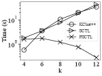
Exp 1 : Runtime of various algorithms with varying $k$ . Figure 4 shows the running time of $\mathsf{KClist}$ ++, $\mathsf{SCTL}$ , and $\mathsf{PSCTL}$ for varying $k$ . To show the advantage of $\mathsf{PBUpdate}$ , we omit the time taken by clique enumeration of $\mathsf{KClist}$ ++ and SCT construction.

As $k$ increases, the running time of $\mathsf{PSCTL}$ tends to be small. This is because the size of the SCT decreases, i.e. the value of $|\mathbb{P}|$ (Theorem 3.8) tends to be small as $k$ increases (Jain and Seshadhri, 2020). For example, on $\mathsf{Pokec}$ , we have $|\mathbb{P}|=10859743$ when $k=4$ , while $|\mathbb{P}|=837568$ when $k=9$ . As shown in Figure 4, $\mathsf{PSCTL}$ substantially outperforms both $\mathsf{KClist}$ ++ and $\mathsf{SCTL}$ when $k=9$ on all the datasets. For example, on $\mathsf{DBLP}$ , our $\mathsf{PSCTL}$ algorithm can achieve more than $5$ orders of magnitude faster than both $\mathsf{KClist}$ ++ and $\mathsf{SCTL}$ when $k\geq 7$ . These results demonstrate the high efficiency of the proposed $\mathsf{PSCTL}$ algorithm.

Additionally, on the complex networks that the degeneracy is larger than $100$ ( $\mathsf{DBLP}$ , $\mathsf{Berkstan}$ and $\mathsf{Skitter}$ in Figure 4), our $\mathsf{PSCTL}$ algorithm can consistently outperform the state-of-the-arts. On these networks, the count of cliques is very large. For example, $\mathsf{Berkstan}$ has $9.4\times 10^{12}$ $7$ -cliques. The excellent performance of $\mathsf{PSCTL}$ is due to the fact that the running time of $\mathsf{PSCTL}$ is free from the count of $k$ -cliques, which confirms our theoretical analysis in Section 3.

Exp 2 : Runtime of various algorithms with varying $T$ . Figure 5 shows the performance of the Frank-Wolfe based algorithms when $T$ varies on Gowalla and Pokec. The results on the other datsets are consistent. We omit the time taken by clique enumeration and SCT construction. As expected, the running time of all algorithms is linear with respect to (w.r.t.) $T$ . Once again, our $\mathsf{PSCTL}$ is much more efficient than the existing algorithms. These results further demonstrate the high efficiency of the proposed solution.

Exp 3 : $k$ -clique density with varying $T$ . In Table 4, only $\mathsf{PSCTL}$ can handle all the tested networks. $\mathsf{KClist}$ ++ can reach to the optimal results in only one iteration, but can not handle the complex networks with a large degeneracy, in which there exists a large number of $k$ -cliques, like $\mathsf{Berkstan}$ . Both $\mathsf{SCTL}$ and $\mathsf{PSCTL}$ can achieve a near-optimal approximation within a few iterations. These results further confirm the scalability of $\mathsf{PSCTL}$ and the ability of $\mathsf{PSCTL}$ to derive a good approximation within only few iterations.

Exp 4 : Running time needed to find $V^{*}$ . In the experiments, we find that $\mathsf{PSCTL}$ can reach $V^{*}$ on all the tested datasets. Table 5 shows the number of iterations as well as the running time needed to find $V^{*}$ . We find that $\mathsf{PSCTL}$ achieves the lowest running time to obtain $V^{*}$ on $6$ datasets. Although $\mathsf{PSCTL}$ requires $110$ iterations to converge to $V^{*}$ on $\mathsf{Youtube}$ , it can get a $99.999\%$ approximation using only $2.0$ seconds. These results further confirm the high efficiency of the proposed $\mathsf{PSCTL}$ algorithm.

Exp 5 : $k$ -clique density within fixed time. Figure 6 compares the $k$ -clique density of the results of $\mathsf{SCTL}$ and $\mathsf{PSCTL}$ with the same running time. In Figure 6, the results show that $\mathsf{PSCTL}$ can get larger $k$ -clique density than $\mathsf{SCTL}$ with the same running time. The results on other datasets is in Table 5 as described in Exp 4.

Exp 6 : Memory overheads. We plot the memory costs of the Frank-Wolfe based algorithms in Figure 7. As can be seen, $\mathsf{PSCTL}$ and $\mathsf{SCTL}$ have similar memory costs. This is because the memory costs of $\mathsf{SCTL}$ and $\mathsf{PSCTL}$ are mainly taken by storing the SCT, while the memory cost of $\mathsf{KClist}$ ++ is by the storage of all $k$ -cliques. As $k$ increases, the count of $k$ -cliques grows and the size of SCT shrinks.These results indicate that our $\mathsf{PSCTL}$ is space-efficient.

5.2. Results of the Sampling-based algorihtms

Exp 7 : Running time with varying $k$ . In Figure 8, we show the running time of the sampling-based algorithms for various values of $k$ . From Figure 8(a) to 8(d), we can see that $\mathsf{CPSample}$ and $\mathsf{SCTSample}$ achieve comparable performance. However, for large networks in Figure 8(e) $\sim$ 8(j), our $\mathsf{CPSample}$ algorithm substantially outperforms $\mathsf{KCLSample}$ and $\mathsf{SCTSample}$ . For example, on the $\mathsf{Pokec}$ dataset, our algorithm is at least one order of magnitude faster than the two baselines. We also note that on the largest graph $\mathsf{Friend}$ , only our algorithm can obtain the results, while both of $\mathsf{KCLSample}$ and $\mathsf{SCTSample}$ fail to drive the results. These results confirm the high efficiency and scalability of our sampling-based algorithm.

Exp 8 : $k$ -clique density within fixed time. In Table 6, we compare $k$ -clique density achieved by the sampling based algorithms within fixed running time. As shown in Table 6, our $\mathsf{CPSample}$ one order of magnitude faster than existing algorithms and achieve good results. For example, on $\mathsf{DBLP}$ , $\mathsf{CPSample}$ can terminate in $0.1s$ while $\mathsf{SCTSample}$ needs around $1s$ and $\mathsf{KCLSample}$ needs about $20s$ . Furthermore, our $\mathsf{CPSample}$ is the only algorithm that can obtain the results on the largest graph $\mathsf{Friend}$ . These results confirm the high efficiency, effectiveness and scalability of our $\mathsf{CPSample}$ .

6. related work

Densest subgraph problem (DSP). Given a graph and a measure of density, DSP requires to find a subset of vertices whose induced subgraph maximizes the value of density. DSP is a famous problem that has been studied for over five decades, which has a lot of variants and applications (Lanciano et al., 2023). For the traditional Edge-based Densest Subgraph Problem, several key algorithmic approaches have emerged. These encompass maximum-flow-based algorithms (Goldberg, 1984), LP-based algorithms (Charikar, 2000b; Danisch et al., 2017) and peeling-based algorithms (Charikar, 2000b; Boob et al., 2020). There are also many variants of DSP. Densest $k$ -subgraph problem aims at finding the densest subgraph with size $k$ (Feige et al., 2001); Densest at-least(most)-k-subgraph problem aims at finding the densest subgraph with size at least(most) $k$ (Andersen and Chellapilla, 2009); Anchored Densest Subgraph Problem tries to find the densest subgraph that contains a given seed set (Dai et al., 2022); Fair densest subgraph is the densest subgraphs that has equal represented colors (Anagnostopoulos et al., 2020; Miyauchi et al., 2023); Motif-based densest subgraph is the generalized version of $k$ -clique densest subgraph, where the density is defined by the count of a given motif (Fang et al., 2019). On different graphs like directed graphs (Charikar, 2000b; Ma et al., 2020), temporal graphs (Bogdanov et al., 2011) and hypergraphs (Huang and Kahng, 1995), there also exists the corresponding DSPs.

Large near-clique detection.The maximum clique problem is an important problem which has a lot of applications (Tomita, 2017; Chang, 2020). However, maximum clique often has a very tight constraints for real-world applications. Thus, a lot of relaxed models for large near-clique detection were proposed (Tsourakakis, 2015; Batagelj and Zaversnik, 2003; Balasundaram et al., 2011; Chen et al., 2021). The $k$ -clique densest subgraph studied in this work is known as a large near-clique. State-of-the-art algorithms for solving $k$ - $\mathsf{DSS}$ are primarily rooted in the Frank-Wolfe framework, because $k$ - $\mathsf{DSS}$ can be formulated as a convex programming. Sun (Sun et al., 2020) introduced the first Frank-Wolfe-based algorithm, named $\mathsf{KClist}$ ++. $\mathsf{KClist}$ ++ operates by sequentially iterating over individual $k$ -cliques, and each $k$ -clique assigns a weight to the vertex with the smallest weight among the $k$ vertices. With an adequate number of iterations, it can converge to the optimal solution $V^{*}$ . Recent advancements by He et al. (He et al., 2023) have accelerated $\mathsf{KClist}$ ++, $\mathsf{KEXACT}$ and $\mathsf{KCLSample}$ by the technique SCT-index. The SCT-index, building upon the SCT-tree data structure (Jain and Seshadhri, 2020), enables batch-wise iteration over $k$ -cliques, significantly enhancing efficiency. Other methods include flow-based algorithms (Mitzenmacher et al., 2015; Tsourakakis, 2015) and peeling-based algorithms (Fang et al., 2019), but they are not as efficient as the Frank-Wolfe based algorithms (He et al., 2023). There also exists a lot of other near-clique models (Batagelj and Zaversnik, 2003; Balasundaram et al., 2011; Chang, 2023). Maximum $k$ -core is the largest subgraph that each vertex has degree larger than $k$ (Batagelj and Zaversnik, 2003). Maximum $k$ -plex is the maximum subgraph that each vertex has at most $k$ non-neighbors (Balasundaram et al., 2011; Chang et al., 2022). Maximum $s$ -defective clique is the maximum subgraph that misses at most $s$ edges compared to clique (Chen et al., 2021; Chang, 2023; Gao et al., 2022).

7. conclusion

In this paper, we study the problem of $k$ -clique densest subgraph search. We propose a new Frank-Wolfe-based algorithm, whose time complexity is free from the count of $k$ -cliques. Thus, it is very efficient for processing large graphs that often have a extremely number of $k$ -cliques. We present a detailed theoretical analysis of our algorithms. To further improve the efficiency, we also propose a new and provable sampling-based algorithm. A nice feature of our algorithm is that it has polynomial time complexity. We conduct extensive experiments on 12 large real-world graphs to evaluate our algorithms, and the results demonstrate the high efficiency and scalability of our approaches.

References

(1)
Anagnostopoulos et al. (2020) Aris Anagnostopoulos, Luca Becchetti, Adriano Fazzone, Cristina Menghini, and Chris Schwiegelshohn. 2020. Spectral Relaxations and Fair Densest Subgraphs. In CIKM. 35–44.
Andersen and Chellapilla (2009) Reid Andersen and Kumar Chellapilla. 2009. Finding Dense Subgraphs with Size Bounds. In WAW, Vol. 5427. Springer, 25–37.
Balasundaram et al. (2011) Balabhaskar Balasundaram, Sergiy Butenko, and Illya V. Hicks. 2011. Clique Relaxations in Social Network Analysis: The Maximum k-Plex Problem. Oper. Res. 59, 1 (2011), 133–142.
Batagelj and Zaversnik (2003) Vladimir Batagelj and Matjaz Zaversnik. 2003. An O(m) Algorithm for Cores Decomposition of Networks. CoRR cs.DS/0310049 (2003).
Bogdanov et al. (2011) Petko Bogdanov, Misael Mongiovì, and Ambuj K. Singh. 2011. Mining Heavy Subgraphs in Time-Evolving Networks. In ICDM. IEEE Computer Society, 81–90.
Boob et al. (2020) Digvijay Boob, Yu Gao, Richard Peng, Saurabh Sawlani, Charalampos E. Tsourakakis, Di Wang, and Junxing Wang. 2020. Flowless: Extracting Densest Subgraphs Without Flow Computations. In WWW. 573–583.
Chang (2020) Lijun Chang. 2020. Efficient maximum clique computation and enumeration over large sparse graphs. VLDB J. 29, 5 (2020), 999–1022.
Chang (2023) Lijun Chang. 2023. Efficient Maximum k-Defective Clique Computation with Improved Time Complexity. CoRR abs/2309.02635 (2023).
Chang et al. (2022) Lijun Chang, Mouyi Xu, and Darren Strash. 2022. Efficient Maximum k-Plex Computation over Large Sparse Graphs. Proc. VLDB Endow. 16, 2 (2022), 127–139.
Charikar (2000a) Moses Charikar. 2000a. Greedy approximation algorithms for finding dense components in a graph. In APPROX 2000, Vol. 1913. Springer, 84–95.
Charikar (2000b) Moses Charikar. 2000b. Greedy approximation algorithms for finding dense components in a graph. In International workshop on approximation algorithms for combinatorial optimization. 84–95.
Chen et al. (2021) Xiaoyu Chen, Yi Zhou, Jin-Kao Hao, and Mingyu Xiao. 2021. Computing maximum k-defective cliques in massive graphs. Comput. Oper. Res. 127 (2021), 105131.
Cui et al. (2008) Guangyu Cui, Yu Chen, De-Shuang Huang, and Kyungsook Han. 2008. An algorithm for finding functional modules and protein complexes in protein-protein interaction networks. Journal of Biomedicine and Biotechnology 2008 (2008).
Dai et al. (2022) Yizhou Dai, Miao Qiao, and Lijun Chang. 2022. Anchored Densest Subgraph. In SIGMOD. 1200–1213.
Danisch et al. (2017) Maximilien Danisch, T.-H. Hubert Chan, and Mauro Sozio. 2017. Large Scale Density-friendly Graph Decomposition via Convex Programming. In WWW 2017. ACM, 233–242.
Eppstein et al. (2013) David Eppstein, Maarten Löffler, and Darren Strash. 2013. Listing All Maximal Cliques in Large Sparse Real-World Graphs. ACM J. Exp. Algorithmics 18 (2013).
Fang et al. (2019) Yixiang Fang, Kaiqiang Yu, Reynold Cheng, Laks V. S. Lakshmanan, and Xuemin Lin. 2019. Efficient Algorithms for Densest Subgraph Discovery. Proc. VLDB Endow. 12, 11 (2019), 1719–1732.
Feige et al. (2001) Uriel Feige, Guy Kortsarz, and David Peleg. 2001. The Dense k-Subgraph Problem. Algorithmica 29, 3 (2001), 410–421.
Fratkin et al. (2006) Eugene Fratkin, Brian T. Naughton, Douglas L. Brutlag, and Serafim Batzoglou. 2006. MotifCut: regulatory motifs finding with maximum density subgraphs. Bioinformatics 22, 14 (07 2006), e150–e157.
Gao et al. (2022) Jian Gao, Zhenghang Xu, Ruizhi Li, and Minghao Yin. 2022. An Exact Algorithm with New Upper Bounds for the Maximum k-Defective Clique Problem in Massive Sparse Graphs. In AAAI. 10174–10183.
Goldberg (1984) Andrew V Goldberg. 1984. Finding a maximum density subgraph. (1984).
He et al. (2023) Yizhang He, Kai Wang, Wenjie Zhang, Xuemin Lin, and Ying Zhang. 2023. Scaling Up k-Clique Densest Subgraph Detection. Proc. ACM Manag. Data 1, 1 (2023), 69:1–69:26.
Huang and Kahng (1995) Dennis J.-H. Huang and Andrew B. Kahng. 1995. When clusters meet partitions: new density-based methods for circuit decomposition. In ED&TC. 60–64.
Jaggi (2013) Martin Jaggi. 2013. Revisiting Frank-Wolfe: Projection-Free Sparse Convex Optimization. In ICML 2013, Vol. 28. 427–435.
Jain and Seshadhri (2020) Shweta Jain and C. Seshadhri. 2020. The Power of Pivoting for Exact Clique Counting. In WSDM. 268–276.
Konar and Sidiropoulos (2022) Aritra Konar and Nicholas D. Sidiropoulos. 2022. The Triangle-Densest-K-Subgraph Problem: Hardness, Lovász Extension, and Application to Document Summarization. Proceedings of the AAAI Conference on Artificial Intelligence 36, 4 (Jun. 2022), 4075–4082.
Lanciano et al. (2023) Tommaso Lanciano, Atsushi Miyauchi, Adriano Fazzone, and Francesco Bonchi. 2023. A Survey on the Densest Subgraph Problem and its Variants. CoRR abs/2303.14467 (2023).
Lee et al. (2010) Victor E. Lee, Ning Ruan, Ruoming Jin, and Charu C. Aggarwal. 2010. A Survey of Algorithms for Dense Subgraph Discovery. In Managing and Mining Graph Data. Advances in Database Systems, Vol. 40. Springer, 303–336.
Li et al. (2022) Rong-Hua Li, Qiushuo Song, Xiaokui Xiao, Lu Qin, Guoren Wang, Jeffrey Xu Yu, and Rui Mao. 2022. I/O-Efficient Algorithms for Degeneracy Computation on Massive Networks. IEEE Transactions on Knowledge and Data Engineering 34, 7 (2022), 3335–3348.
Ma et al. (2020) Chenhao Ma, Yixiang Fang, Reynold Cheng, Laks VS Lakshmanan, Wenjie Zhang, and Xuemin Lin. 2020. Efficient algorithms for densest subgraph discovery on large directed graphs. In SIGMOD. 1051–1066.
Mitzenmacher et al. (2015) Michael Mitzenmacher, Jakub Pachocki, Richard Peng, Charalampos E. Tsourakakis, and Shen Chen Xu. 2015. Scalable Large Near-Clique Detection in Large-Scale Networks via Sampling. In SIGKDD 2015. ACM, 815–824.
Miyauchi et al. (2023) Atsushi Miyauchi, Tianyi Chen, Konstantinos Sotiropoulos, and Charalampos E. Tsourakakis. 2023. Densest Diverse Subgraphs: How to Plan a Successful Cocktail Party with Diversity. In SIGKDD. 1710–1721.
Sun et al. (2020) Bintao Sun, Maximilien Danisch, T.-H. Hubert Chan, and Mauro Sozio. 2020. KClist++: A Simple Algorithm for k-Clique Densest Subgraphs in Large Graphs. Proc. VLDB Endow. 13, 10 (2020), 1628–1640.
Tomita (2017) Etsuji Tomita. 2017. Efficient Algorithms for Finding Maximum and Maximal Cliques and Their Applications. In WALCOM, Vol. 10167. Springer, 3–15.
Tsourakakis (2015) Charalampos E. Tsourakakis. 2015. The K-clique Densest Subgraph Problem. In WWW. 1122–1132.
Ye et al. (2022) Xiaowei Ye, Rong-Hua Li, Qiangqiang Dai, Hongzhi Chen, and Guoren Wang. 2022. Lightning Fast and Space Efficient k-clique Counting. In WWW. 1191–1202.
Yu et al. (2006) Haiyuan Yu, Alberto Paccanaro, Valery Trifonov, and Mark Gerstein. 2006. Predicting interactions in protein networks by completing defective cliques. Bioinform. 22, 7 (2006), 823–829.

Scalable kk-clique Densest Subgraph Search

Abstract.

1. Introduction

Example 1.1.

2. Preliminaries

Definition 2.1 (kk-clique Densest Subgraph).

Lemma 2.2 ((Sun et al., 2020)).

Lemma 2.3 ((Sun et al., 2020; Danisch et al., 2017)).

Lemma 2.4 ((Jain and Seshadhri, 2020)).

Lemma 2.5.

Proof.

Lemma 2.6 ((Jain and Seshadhri, 2020)).

Example 2.7.

3. New Convex Programming for kk-DSS

3.1. SCT-based Convex Programming

Lemma 3.1.

Proof.

Theorem 3.2.

Proof.

Definition 3.3.

Theorem 3.4.

Proof.

Theorem 3.5.

Proof.

Theorem 3.6.

Proof.

Theorem 3.7.

Proof.

3.2. FW-based Algorithm for SCT-CP(G)

Theorem 3.8.

Proof.

Example 3.9.

3.3. Analysis of the Algorithm

Theorem 3.10.

Proof.

Corollary 3.11.

Lemma 3.12.

Proof.

Theorem 3.13.

Proof.

Theorem 3.14.

Proof.

4. New Sampling-Based Algorithm

4.1. The 𝖢𝖯𝖲𝖺𝗆𝗉𝗅𝖾\mathsf{CPSample} algorithm

Theorem 4.1.

Proof.

4.2. Analysis of the Algorithm

Theorem 4.2 (Chernoff bound).

Lemma 4.3.

Proof.

Lemma 4.4.

Proof.

Theorem 4.5.

Proof.

Theorem 4.6.

Proof.

5. Experiments

5.1. Results of the FW-based algorihtms

5.2. Results of the Sampling-based algorihtms

6. related work

7. conclusion

References

Scalable $k$ -clique Densest Subgraph Search

Definition 2.1 ( $k$ -clique Densest Subgraph).

3. New Convex Programming for $k$ -DSS

4.1. The $\mathsf{CPSample}$ algorithm