Scalable iterative data-adaptive RKHS regularization
Abstract
We present iDARR, a scalable iterative Data-Adaptive RKHS Regularization method, for solving ill-posed linear inverse problems. The method searches for solutions in subspaces where the true solution can be identified, with the data-adaptive RKHS penalizing the spaces of small singular values. At the core of the method is a new generalized Golub-Kahan bidiagonalization procedure that recursively constructs orthonormal bases for a sequence of RKHS-restricted Krylov subspaces. The method is scalable with a complexity of for -by- matrices with denoting the iteration numbers. Numerical tests on the Fredholm integral equation and 2D image deblurring show that it outperforms the widely used and norms, producing stable accurate solutions consistently converging when the noise level decays.
Keywords: iterative regularization; ill-posed inverse problem; reproducing kernel Hilbert space; Golub-Kahan bidiagonalization; deconvolution.
AMS subject classifications(MSC2020): 47A52, 65F22, 65J20
1 Introduction
This study considers large-scale ill-posed linear inverse problems with little prior information on the regularization norm. The goal is to reliably solve high-dimensional vectors from the equation
| (1.1) |
where and are data-dependent forward mapping and output, and denotes noise or measurement error. The problem is ill-posed in the sense that the least squares solution with minimal Euclidean norm, often solved by or with † denoting pseudo-inverse, is sensitive to perturbations in . Such an ill-posedness happens when the singular values of decay to zero faster than the perturbation in projected in the corresponding singular vectors.
Regularization is crucial to producing stable solutions for the ill-posed inverse problem. Broadly, it encompasses two integral components: a penalty term that defines the search domain and a hyperparameter that controls the strength of regularization. There are two primary approaches to implementing regularization: direct methods, which rely on matrix decomposition, e.g., the Tikhonov regularization [35], the truncated singular value decomposition (SVD) [15, 11]; and iterative methods, which use matrix-vector computations to scale for high-dimensional problems, see e.g., [12, 7, 41] for recent developments.
In our setting, we encounter two primary challenges: selecting an adaptive regularization norm and devising an iterative method to ensure scalability. The need for an adaptive norm arises from the variability of the forward map across different applications and the often limited prior information about the regularity of . Many existing regularization norms, such as the Euclidean norms used in Tikhonov methods in [15, 35] and the total variation norm in [33], lack this adaptability; for more examples, see the related work section below. Although a data-adaptive regularization norm has been proposed in [26, 25] for nonparametric regression, it is implicitly defined and requires a spectral decomposition of the normal operator.
We introduce iDARR, an iterative Data-Adaptive Reproducing kernel Hilbert space Regularization method. This method resolves both challenges by iteratively solving the subspace-projected problem
where is the implicitly defined semi-norm of a data-adaptive RKHS (DA-RKHS), and are subspaces of the DA-RKHS constructed by a generalized Golub-Kahan bidiagonalization (gGKB). By stopping the iteration early using the L-curve criterion, it produces a stable accurate solution without using any matrix decomposition.
The DA-RKHS is a space defined by the data and model, embodying the intrinsic nature of the inverse problem. Its closure is the data-dependent space in which the true solution can be recovered, particularly when is deficient-ranked. Thus, when used for regularization, it confines the solution search in the right space and penalizes the small singular values, leading to stable solutions. We construct this DA-RKHS by reformulating eq. 1.1 as a weighted Fredholm integral equation of the first kind and examining the identifiability of the input signal, as detailed in Section 2.
Our key innovation is the gGKB. It constructs solution subspaces in the DA-RKHS without explicitly computing it. It is scalable with a cost of only , where is the number of iterations. This cost is orders of magnitude much smaller than the cost of direct methods based on spectral decomposition of , typically operations.
The iDARR and gGKB have solid mathematical foundations. We prove that each subspace is restricted in the DA-RKHS, thereby named the RKHS-restricted Krylov subspaces. It is spanned by the orthonormal vectors produced by gGKB. Importantly, if not stopped early, the gGKB terminates when the RKHS-restricted Krylov subspace is fully explored, and the solution in each iteration is unique.
Systematic numerical tests employing the Fredholm integral equations demonstrate that iDARR surpasses traditional iterative methods employing and norms in the state-of-the-art IR TOOLS package [12]. Notably, iDARR delivers accurate estimators that consistently decay with the noise level. This superior performance is evident irrespective of whether the spectral decay is exponential or polynomial, or whether the true solution resides inside or outside the DA-RKHS. Furthermore, our application to image deblurring underscores both its scalability and accuracy.
Main contributions. Our main contribution lies in developing iDARR, a scalable iterative regularization method tailored for large-scale ill-posed inverse problems with little prior knowledge about the solution. The cornerstone of iDARR is the introduction of a new data-adaptive RKHS determined by the underlying model and the data. A key technical innovation is the gGKB, which efficiently constructs solution subspaces of the implicitly defined DA-RKHS.
1.1 Related work
Numerous regularization methods have been developed, and the literature on this topic is too vast to be surveyed here; we refer to [15, 11, 12] and references therein for an overview. In the following, we compare iDARR with the most closely related works.
Regularization norms
Various regularization norms exist, such as Euclidean norms of Tikhonov in [15, 35], the total variation norm of the Rudin–Osher–Fatemi method in [33], the norm of LASSO in [34], and the RKHS norm of an RKHS with a user-specified reproducing kernel [37, 3, 9]. These norms, however, are often based on presumed properties of the solution and do not consider the specifics of each inverse problem. Our RKHS norm differs by adapting to the model and data: our RKHS has a reproducing kernel determined by the inverse problem, and its closure is the space in which the solution can be identified, making it an apt choice for regularization in the absence of additional solution information.
Iterative regularization (IR) methods
IR methods are scalable by accessing the matrix only via matrix-vector multiplications, producing a sequence of estimators until an early stopping, where the iteration number plays the role of the regularization parameter. IR has a rich and extensive history and continues to be a vibrant area of interest in contemporary studies [30, 1, 12, 24]. Different regularization terms lead to various methods. The LSQR algorithm [30, 5] with early stopping is standard for -regularization. It solves projected problems in Krylov subspaces before transforming back to the original domain. For with , the widely-used methods include joint bidiagonalization method [19, 18], generalized Krylov subspace method [21, 31], random SVD or generalized SVD method [39, 40, 38], modified truncated SVD method [2, 17], etc. For the general regularization norm in the form with a symmetric matrix , the MLSQR in [1] treats positive definite and the preconditioned GKB [24] handles positive semi-definite ’s. Our iDARR studies the case that is unavailable but is ready to be used.
Golub-Kahan bidiagonalization (GKB)
The GKB was first used to solve inverse problems in [29], which generates orthonormal bases for Krylov subspaces in and . This method extends to bounded linear compact operators between Hilbert spaces, with properties and convergence results detailed in [6]. Our gGKB extends the method to construct RKHS-restricted Krylov subspace in and , where is positive semidefinite, and in particular, only is available.
The remainder of this paper is organized as follows: Section 2 introduces the adaptive RKHS with a characterization of its norm. Section 3 presents in detail the iDARR. Section 4 proves the desired properties of gGKB. In Section 5, we systematically examine the algorithm and demonstrate the robust convergence of the estimator when the noise becomes small. Finally, Section 6 concludes with a discussion on future developments.
2 A Data Adaptive RKHS for Regularization
This section introduces a data-adaptive RKHS (DA-RKHS) that adapts to the model and data in the inverse problem. The closure of this DA-RKHS is the function (or vector) space in which the true solution can be recovered, or equivalently, the inverse problem is well-defined in the sense that the loss function has a unique minimizer. Hence, when its norm is used for regularization, this DA-RKHS ensures that the minimization searches in the space where we can identify the solution.
To describe the DA-RKHS, we first present a unified notation that applies to both discrete and continuous time models using a weighted Fredholm integral equation of the first kind. Based on this notation, we write the normal operator as an integral operator emerging in a variational formulation of the inverse problem. The integral kernel is the reproducing kernel for the DA-RKHS. In other words, the normal operator defines the DA-RKHS. At last, we briefly review a DA-RKHS Tikhonov regularization algorithm, the DARTR algorithm.
2.1 Unified notation for discrete and continuous models
The linear equation eq. 1.1 can arise from discrete or continuous inverse problems. In either case, we can present the inverse problem using the prototype of the Fredholm integral equation of the first kind. We consider only the 1D case for simplicity, and the extension to high-dimensional cases is straightforward. Specifically, let be two compact sets. We aim to recover the function in the Fredholm equation
| (2.1) |
from discrete noisy data
where we assume the observation index to be for simplicity. Here the measurement noise is the white noise scaled by ; that is, the noise at has a Gaussian distribution for each . Such noise is integrable when the observation mesh refines, i.e., vanishes.
Here the finite measure can be either the Lebesgue measure with being an interval or an atom measure with having finitely many elements. Correspondingly, the Fredholm integral equation eq. 2.1 is either a continuous or a discrete model.
In either case, the goal is to solve for the function in eq. 2.1. When seeking a solution in the form of , where is a pre-selected set of basis functions, we obtain the linear equation eq. 1.1 with and the matrix with entries
| (2.2) |
In particular, when are piece-wise constants, we obtain as follows.
-
•
Discrete model. Let be an atom measure on , a set with elements. Suppose that the basis functions are . Then, and the matrix has entries .
-
•
Continuous model. Let be the Lebesgue measure on , and be piecewise constant functions on a partition of with . Then, and the matrix has entries .
The default function spaces for and above are and . The loss function over becomes
| (2.3) |
Eq.eq. 2.1 is a prototype of ill-posed inverse problems, dating back from Hadamard [14], and it remains a testbed for new regularization methods [36, 28, 15, 23].
The norm is often a default choice for regularization. However, it has a major drawback: it does not take into account the operator , particularly when has zero eigenvalues, and it leads to unstable solutions that may blow up in the small noise limit [22]. To avoid such instability, particularly for iterative methods, we introduce a weighted function space and an RKHS that are adaptive to both the data and the model in the next sections.
2.2 The function space of identifiability
We first introduce a weighted function space , where the measure is defined as
| (2.4) |
where is a normalizing constant. This measure quantifies the exploration of data to the unknown function through the integral kernel at the output set , i.e., , hence it is referred to as an exploration measure. In particular, when (1.1) is a discrete model, the exploration measure is the normalized column sum of the absolute values of the matrix .
The major advantage of the space over the original space is that it is adaptive to the specific setting of the inverse problem. In particular, this weighted space takes into account the structure of the integral kernel and the data points in . Thus, while the following introduction of RKHS can be carried out in both and , we will focus only on .
Next, we consider the variational inverse problem over , and the goal is to find a minimizer of the loss function eq. 2.3 in . Since the loss function is quadratic, its Hessian is a symmetric positive linear operator, and it has a unique minimizer in the linear subspace where the Hessian is strictly positive. We assign a name to this subspace in the next definition.
Definition 2.1 (Function space of identifiability)
In a variational inverse problem of minimizing a quadratic loss function in , we call the normal operator, where is the Hessian of , and we call the function space of identifiability (FSOI).
Lemma 2.2
Assume . For in eq. 2.4, define as
| (2.5) |
-
(a)
The normal operator for in eq. 2.3 over is defined by
(2.6) and the loss function can be written as
(2.7) where comes from Riesz representation s.t. for any .
-
(b)
is compact, self-adjoint, and positive. Hence, its eigenvalues converge to zero and its orthonormal eigenfunctions form a complete basis of .
-
(c)
The FSOI is , and the unique minimizer of in H is , where is the inversion of .
Lemma 2.2 reveals the cause of the ill-posedness, and provides insights on regularization:
-
•
The variational inverse problem is well-defined only in the FSOI , which can be a proper subset of . Its ill-posedness in depends on the smallest eigenvalue of the operator and the error in .
-
•
When the data is noiseless, the loss function can only identify the -projection of the true input function. When data is noisy, its minimizer is ill-defined in when .
As a result, when regularizing the ill-posed problem, an important task is to ensure the search takes place in the FSOI and to remove the noise-contaminated components making .
2.3 A Data-adaptive RKHS
Our data-adaptive RKHS is the RKHS with in eq. 2.5 as a reproducing kernel. Hence, it is adaptive to the integral kernel and the data in the model. When its norm is used for regularization, it ensures that the search takes place in the FSOI because its closure is the FSOI; also, it penalizes the components in corresponding to the small singular values.
The next lemma characterizes this RKHS, and we refer to [26] for its proof.
Lemma 2.3 (Characterization of the adaptive RKHS)
Assume . The RKHS with as its reproducing kernel satisfies the following properties.
-
(a)
has inner product
-
(b)
is an orthonormal basis of , where are eigen-pairs of .
-
(c)
For any , we have
-
(d)
with inclosure in , where is the FSOI.
The next theorem shows the computation of the RKHS norm for the problem eq. 1.1 when it is written in the form eq. 2.1-eq. 2.2. A key component is solving the eigenvalues of through a generalized eigenvalue problem.
Theorem 2.4 (Computation of RKHS norm)
Suppose that eq. 1.1 is equivalent to eq. 2.1 under basis functions with and eq. 2.2. Let with entries be the non-singular basis matrix, where is the measure defined in eq. 2.4. Then, the operator in eq. 2.6 has eigenvalues solved by the generalize eigenvalue problem:
| (2.8) |
and the eigenfunctions are . The RKHS norm of satisfies
| (2.9) | ||||
In particular, if , we have .
Proof. Denote and . We first prove that the eigenvalues of are solved by eq. 2.8. We suppose are the eigenvalues and eigen-functions of over with being an orthonormal basis of . Since , there exists such that , i.e., for each . Then, the task is to verify that and satisfy and .
The orthonormality of implies that
Note that for . Then,
Meanwhile, the eigen-equation implies that for each ,
i.e., . Hence, these two equations imply that .
Next, to compute the norm of , we write it as . Then, its norm is
Thus, and .
In particular, when eq. 1.1 is either a discrete model or a discretization of eq. 2.1 based on Riemann sum approximation of the integral, the exploration measure is the normalized column sum of the absolute values of the matrix , and . See Section 5.1 for details.
2.4 DARTR: data-adaptive RKHS Tikhonov regularization
We review DARTR, a data-adaptive RKHS Tikhonov regularization algorithm introduced in [26].
Specifically, it solves the problem eq. 1.1 with regularization:
where the norm is the DA-RKHS norm introduced in Theorem 2.4. A direct solution minimizing is to solve . However, the computation of requires a pseudo-inverse that may cause numerical instability.
DARTR introduces a transformation matrix to avoid using the pseudo-inverse. Note that , where is the identity matrix with rank , the number of positive eigenvalues in . Then, the linear equation is equivalent to
| (2.10) |
with . Thus, DARTR computes in the above equation by least squares with minimal norm, and returns .
DARTR is a direct method based on matrix decomposition, and it takes flops. Hence, it is computationally infeasible when is large. The iterative method in the next section implements the RKHS regularization in a scalable fashion.
3 Iterative Regularization by DA-RKHS
This section introduces a subspace project method tailored to utilize the DA-RKHS for iterative regularization. As an iterative method, it achieves scalability by accessing the coefficient matrix only via matrix-vector multiplications, producing a sequence of estimators until reaching a desired solution. This section follows the notation conventions in Table 1.
| matrix or array by capital letters | |
|---|---|
| vector by regular letters | |
| scalar by Greek letters | |
| and | the range and null spaces of matrix |
3.1 Overview
Our regularization method is based on subspace projection in the DA-RKHS. It iteratively constructs a sequence of linear subspaces of the DA-RKHS , and recursively solves projected problems
| (3.1) |
This process yields a sequence of solutions , each emerging from its corresponding subspace. We ensure the uniqueness of the solution within each iteration, as detailed in Theorem 4.7. The iteration proceeds until it meets an early stopping criterion, designed to exclude excessive noisy components and thereby achieve effective regularization. The spaces are called the solution subspaces, and the iteration number plays the role of the regularization parameter.
Algorithm 1 outlines this procedure, which is a recursion of the following three parts.
-
P1
Construct the solution subspaces. We introduce a new generalized Golub-Kahan bidiagonalization (gGKB) to construct the solution subspaces in the DA-RKHS iteratively. The procedure is presented in Algorithm 2.
-
P2
Recursively update the solution to the projected problem. We solve the least squares problem in the solution subspaces in eq. 3.1 efficiently by a new LSQR-type algorithm, Algorithm 3, updating and the residual norm without even computing the residual.
-
P3
Regularize by early stopping. We select the optimal by either the discrepancy principle (DP) when we have an accurate estimate of or the L-curve criterion otherwise.
Require: , , , , , where is the exploration measure in eq. 2.4.
Ensure: Final solution
In the next subsection, we present details for these key parts. Then, we analyze the computational complexity of the algorithm.
3.2 Algorithm details and derivations
This subsection presents detailed derivations for the three parts P1-P3 in Algorithm 1.
P1. Construct the solution subspaces. We construct the solution subspaces by elaborately incorporating the regularization term in the Golub-Kahan bidiagonalization (GKB) process. A key point is to use to avoid explicitly computing , which involves the costly spectral decomposition of the normal operator, see eq. 2.9 in Theorem 2.4.
Consider first the case where is positive definite. In this scenario, has full column rank, and the -inner product Hilbert space is a discrete representation of the RKHS with the given basis functions. Note that the true solution is mapped to the noisy by . Let be the adjoint of , i.e. for any and . By definition, the matrix-form expression of is
| (3.2) |
since and for any and .
The Golub-Kahan bidiagonalization (GKB) process recursively constructs orthonormal bases for these two Hilbert spaces starting with the vector as follows:
| (3.3a) | |||
| (3.3b) | |||
| (3.3c) | |||
where , with , and , are normalizing factor such that . The iteration starts with with . Using in eq. 3.2, we write eq. 3.3c as
| (3.4) |
with . To compute without explicitly computing , define . Then we have
| (3.5) |
where . Let . Then we obtain , which uses without computing .
Next, consider that is positive semidefinite. The iterative process remains the same with replaced by the pseudo-inverse , because has the same form as for the non-singular case. Specifically, the recursive relation eq. 3.4 becomes
| (3.6) |
To compute , we use the property that , which will be proved in Proposition 4.3. Note that since is symmetric, where is the projection operator onto subspace . It follows that . Therefore, eq. 3.6 becomes
Letting and again, we get .
Thus, the two cases of lead to the same iterative process. We summarize the iterative process in Algorithm 2, and call it generalized Golub-Kahan bidiagonalization (gGKB).
Require: , ,
Ensure: ,
Suppose the gGKB process terminates at step . We show in Proposition 4.4–Proposition 4.5 that the output vectors and are orthonormal in and , respectively. In particular, they span two Krylov subspaces generated by and , respectively.
In matrix form, the -step gGKB process with , starting with vector , produces a -orthonormal matrix (i.e., ), a -orthonormal matrix , and a bidiagonal matrix
| (3.7) |
such that the recursion in eq. 3.3a,eq. 3.3b and eq. 3.6 can be written as
| (3.8a) | |||
| (3.8b) | |||
| (3.8c) | |||
where and are the first and -th columns of . We emphasize that is a bidiagonal matrix of full column rank, since for all .
P2. Recursively update the solution to the projected problem. For each , i.e., before the gGKB terminates, we solve eq. 3.1 in the subspace
| (3.9) |
and compute the RKHS norm of the solution.
We show first the uniqueness of the solution to eq. 3.1. From eq. 3.8b we have , which implies that is a projection of onto the two subspaces and . Since any vector in can be written as with a , we obtain from eq. 3.8a and eq. 3.8b that for any ,
| (3.10) | ||||
Since , has full column rank, this -dimensional least squares problem has a unique solution. Therefore, the unique solution to eq. 3.1 is
| (3.11) |
We note that the above uniqueness is independent of the specific construction of the basis vectors . In general, as long as , the solution to eq. 3.1 is unique; see Theorem 4.7.
Importantly, we recursively compute without explicitly solving in eq. 3.11, avoiding the computational cost. To this end, we adopt a procedure similar to the LSQR algorithm in [30] to iteratively update from . It starts from the following Givens QR factorization:
where the orthogonal matrix is the product of a series of Givens rotation matrices, and is a bidiagonal upper triangular matrix; see [13, §5.2.5]. We implement the Givens QR factorization using the procedure in [30], which recursively zeros out the subdiagonal elements for each . Specifically, at the -th step, a Givens rotation zeros out by
where the entries and of the Givens rotations satisfy , and the elements , , , , are recursively updated accordingly; see [30] for more details.
As a result of the QR factorization, we can write
| (3.12) |
Hence, the solution to is . Factorizing as
and denoting , we get
Updating recursively, and solving by back substitution, we obtain:
| (3.13) |
Lastly, we compute without an explicit . We have from eq. 3.13:
Letting and , and recalling that , we have
| (3.14) |
The whole updating procedure is described in Algorithm 3. This algorithm yields the residual norm without explicitly computing the residual. In fact, by eq. 3.10 and eq. 3.12 we have
| (3.15) |
Note that decreases monotonically since minimizes in the gradually expanding subspace .
Importantly, Algorithm 3 efficiently computes the solution and . At each step of updating or , the computation takes flops. Similarly, for updating or , as well as for computing , the number of flops are also . Therefore, the dominant computational cost is . In contrast, if is solved explicitly at each step, it takes flops; together with the step of forming that takes flops, they lead to a total cost of flops. Thus, the LSQR-type iteration in Algorithm 3 significantly reduces the number of flops from to .
P3. Regularize by early stopping. An early stopping strategy is imperative to prevent the solution subspace from becoming excessively large, which could otherwise compromise the regularization. This necessity is rooted in the phenomenon of semi-convergence: the iteration vector initially approaches an optimal regularized solution but subsequently moves towards the unstable naive solution to , as detailed in Proposition 4.6.
For early stopping, we adopt the L-curve criterion, as outlined in [12]. This method identifies the ideal early stopping iteration at the corner of the curve represented by
| (3.16) |
Here and are computed with negligible cost in Algorithm 3. To construct the L-curve effectively, we set the gGKB to execute at least 10 iterations. Additionally, to enhance numerical stability, we stop the gGKB when either or is near the machine precision, as inspired by Proposition 4.6.
It is noteworthy that the discrepancy principle (DP) presents a viable alternative when the measurement error in eq. 1.1 is available with a high degree of accuracy. The DP halts iterations at the earliest instance of that satisfies where is chosen to be marginally greater than 1.
3.3 Computational Complexity
Suppose the algorithm takes iterations and the basis matrix is diagonal. Recall that , , and . The total computational cost of Algorithm 1 is about when or ; and about when otherwise. The cost is dominated by the gGKB process since the cost of the update procedure in Algorithm 3 is only at each step.
The gGKB can be computed in two approaches. The first approach uses only matrix-vector multiplication. The main computations in each iteration of gGKB occur at the matrix-vector products and , which take and flops respectively. Thus, the total computational cost of gGKB is flops. Another approach is using instead of and to compute . In this approach, the computation of from takes flops, and the matrix-vector multiplication in each iteration takes about flops. Hence, the total cost of iterations is . The second approach is faster when , or equivalently, . That is, roughly speaking, and .
In practice, the matrix-vector computation is preferred since the iteration number is often small. The resulting iDARR algorithm takes about flops.
4 Properties of gGKB
This section studies the properties of the gGKB in Algorithm 2, including the structure of the solution subspace, the orthogonality of the resulted vectors and and the number of iterations at termination, defined as:
| (4.1) |
Additionally, we show that the solution to eq. 3.1 is unique in each iteration.
Throughout this section, let denote the rank of and let denote the first columns of , where and are matrices constituted by the generalized eigenvalues and eigenvectors of in eq. 2.9 in Theorem 2.4. We have . Recall that . Note that the DA-RKHS is .
4.1 Properties of gGKB
We show first that the gGKB-produced vectors and are orthogonal in and in the DA-RKHS, and the solution subspaces of the gGKB are RKHS-restricted Krylov subspaces.
Definition 4.1 (RKHS-restricted Krylov subspace)
Let and , and let be a symmetric positive definite matrix. Let , which defines an RKHS . The RKHS-restricted Krylov subspaces are
| (4.2) |
The main result is the following.
Theorem 4.2 (Properties of gGKB)
Recall in eq. 4.1, and the gGKB generates vectors , and . They satisfy the following properties:
-
(i)
and are orthonormal in and in , respectively;
-
(ii)
for each , and the termination iteration number is .
Proof. Part (i) follows from Proposition 4.3, where we show that , and Proposition 4.4, where we show the orthogonality of these vectors.
For Part (ii), follows from that form an orthonormal basis of the RKHS-restricted Krylov subspace. We prove in Proposition 4.5.
Proposition 4.3
For each generatad by gGKB in eq. 3.3, it holds that . Additionally, if , then .
Proof. We prove it by mathematical induction. For , we obtain from eq. 3.6 and Theorem 2.4 that , where is the rank of . Suppose for . Using again eq. 3.6 and Theorem 2.4 we get
Therefore, , and .
If , then . Therefore, .
Thus, even if is singular (positive semidefinite), the gGKB in Algorithm 2 does not terminate as long as the right-hand sides of eq. 3.3b and eq. 3.6 are nonzero, since the iterative computation of and can continue. Next, we show that these vectors are orthogonal.
Proposition 4.4 (Orthogonality)
Suppose the -step gGKB does not terminate, i.e. , then is a 2-orthonormal basis of the Krylov subspace
| (4.3) |
and is a -orthonormal basis for the RKHS-restricted Krylov subspace in eq. 4.2.
Proof. Note from Theorem 2.4 that . Let . Then , , and . For any , Proposition 4.3 implies that there exists such that . We get from eq. 3.3b and eq. 3.6 that
where the second equation comes from . Combining the above two relations with eq. 3.3a, we conclude that the iterative process for generating and is the standard GKB process of with starting vector between the two finite dimensional Hilbert spaces and . Therefore, and are two 2-orthonormal bases of the Krylov subspaces
respectively; see e.g. [13, §10.4]. Then, implies eq. 4.3. Also, is a -orthonormal basis of since is -orthonormal.
Finally, are orthogonal by construction, and by using the relation
we get that in the RKHS-restricted Krylov subspace in eq. 4.2.
Proposition 4.5 (gGKB termination number)
Suppose the gGKB in Algorithm 2 terminates at step . Let the distinct nonzero eigenvalues of be with multiplicities , and the corresponding eigenspaces are . Then, , where is the number of nonzero elements in , and
| (4.4) |
where denotes the Krylov subspace of . Moreover, with being the rank of and .
Proof. First, we prove eq. 4.4 with being the number of nonzero elements in . Let for , and let without loss of generality. Note that are orthonormal. Let be a matrix with orthonormal columns that span . Note that . By the eigenvalue decomposition , we have
| (4.5) |
Hence, . On the other hand, for , setting , we have with
where consists of the first rows of , and consists of the rest rows. Note that is a Vandermonde matrix and it is nonsingular since for . Then, has full column rank, thereby the rank of is for , and . Therefore, we have .
Also, we have , where the first equality follows from
| (4.6) |
and the second equality follows from since is non-singular on , which is a subset of by eq. 4.5. In fact, is non-singular on because are eigenspaces of corresponding to the positive eiengvalues.
Furthermore, eq. 4.6 and the non-degeneracy of on imply that
| (4.7) | ||||
That is, the vectors are linearly independent.
Next, we prove that . Clearly, since by Proposition 4.4 are orthogonal and they are in , whose dimension is . On the other hand, we show next that if , there will be a contradiction; hence, we must have . In fact, eq. 3.3b and eq. 3.6 imply that, for each ,
which leads to
Note that . Combining the above two relations and using for all , it follows that for all . Hence, recursively applying for all , we can write
with and in particular, . Now implies that are linearly dependent, contradicting with the fact that they are linearly independent as suggested by eq. 4.7. Therefore, we have .
Lastly, to prove that , it suffices to show that since the eigenvalues of are nonnegative. To see that its rank is , following the proof of Proposition 4.4, we write . Since , we only need to prove that has full column rank. Suppose with . By Theorem 2.4 it follows . Thus, .
4.2 Uniqueness of solutions in the iterations
Proposition 4.6
If gGKB terminates at step in eq. 4.1, the iterative solution is the unique least squares solution to .
Proof. Following the proof of Proposition 4.4, the solution to is with . Since has full column rank, it follows that is the unique solution to . Note that . Thus, is the solution to if and only if .
Now we only need to prove since by Proposition 4.5. Using the property , we get from eq. 3.8c
Combining the above relation with eq. 3.10, we have
since when gGKB terminates.
This result shows the necessity for early stopping the iteration to avoid getting a naive solution. The next theorem shows the uniqueness of the solution in each iteration of the algorithm.
Theorem 4.7 (Uniquess of solution in each iteration)
For each iteration with , there exists a unique solution to eq. 3.1. Furthermore, there exists a unique solution to .
Proof. Let that has orthonormal columns and spans . For any , there is a unique such that . Then the solution to eq. 3.1 should be , where is the solution to
By [10, Theorem 2.1], it has a unique solution iff .
Now we prove . To this end, suppose and . Then . Since , we get . Therefore, , which leads to .
To prove the uniqueness of a solution to , suppose that there are two minimizers, , and we prove that they must be the same. Let and we have since the minimizer of must satisfy . That is, .
On the other hand, since by Proposition 4.3, and note that , we have .
Combining the above two, we have . But is a symmetric positive definite matrix, so we must have .
5 Numerical Examples
5.1 The Fredholm equation of the first kind
We first examine the iDARR in solving the discrete Fredholm integral equation of the first kind. The tests cover two distinct types of spectral decay: exponential and polynomial. The latter is well-known to be challenging, often occurring in applications such as image deblurring. Additionally, we investigate two scenarios concerning whether the true solution is inside or outside the function space of identifiability (FSOI).
Three norms in iterative and direct methods. We compare the , , and DA-RKHS norms in iterative and direct methods. The direct methods are based on matrix decomposition. These regularizers are listed in Table 2.
| Norms | Iterative | Direct | |
|---|---|---|---|
| IR-l2 | l2 | ||
| IR-L2 | L2 | ||
| DA-RKHS | iDARR | DARTR |
The iterative methods differ primarily in their regularization norms. For the with norm, we use the LSQR method in the IR TOOLS package [12], and we stop the iteration when or becomes negligible to maintain stability. For the norm, we use gGKB to construct solution subspaces by replacing by the basis matrix ; note that this method is equivalent to the LSQR method using as a preconditioner in the IR TOOLS package.
The direct methods are Tikhonov regularizers using the L-curve method [16].
Numerical settings. We consider the problem of recovering the input signal in a discretization of Fredholm integral equation in eq. 2.1 with and . The data are discrete noisy observations , where for . The task is to estimate the coefficient vector in a piecewise-constant function , where with , . We obtain the linear system eq. 1.1 with by a Riemann sum approximation of the integral. We set , , and take except when testing the computational time with a sequence of large values for .
The -valued noise is Gaussian . We set the standard deviation of the noise to be , where is the noise-to-signal ratio, and we test our methods with .
We consider two integral kernels
| (5.1) |
which lead to exponential and polynomial decaying spectra, respectively, as shown in Figure 1. The first kernel arises from magnetic resonance relaxometry [4] with being the distribution of transverse nuclear relaxation times.


The DA-RKHS. By its definition in eq. 2.4, the exploration measure is for with being the normalizing constant. In other words, it is the normalized column sum of the absolute values of the matrix . The discrete function space is equivalent to with weight , and its norm is for all . The basis matrix for the Cartesian basis of is , which is also the basis matrix for step functions in the Riemann sum discretization. The DA-RKHS in this discrete setting is .
Settings for comparisons. The comparison consists of two scenarios regarding whether the true solution is inside or outside of the FSOI: (i) the true solution is the second eigenvector of ; thus it is inside the FSOI; and (ii) the true solution is , which has significant components outside the FSOI.
For each scenario, we conduct 100 independent simulations, with each simulation comprising five datasets at varying noise levels. The results are presented by a box plot, which illustrates the median, the lower and upper quartiles, any outliers, and the range of values excluding outliers. The key indicator of a regularizer’s effectiveness is its ability to produce accurate estimators whose errors decay consistently as the noise level decreases. Since exploring the decay rate in the small noise limit is not the focus of this study, we direct readers to [27, 22] for initial insights into how this rate is influenced by factors such as spectral decay, the smoothness of the true solution, and the choice of regularization strength.

Results. We report the results separately according to the spectral decay.
(i) Exponential decaying spectrum. Figure 2’s top row shows typical estimators of IR-l2, IR-L2, and iDARR and their de-noising of the output signal when . When the true solution is inside the FSOI, the iDARR significantly outperforms the other two in producing a more accurate estimator. However, both IR-L2 and IR-l2 can denoise the data accurately, even though their estimators are largely biased. When the true solution is outside the FSOI, all the regularizers can not capture the true function accurately, but iDARR and IR-L2 clearly outperform the regularizer. Yet again, all these largely biased estimators can de-noise the data accurately. Thus, this inverse problem is severely ill-defined, and one must restrict the inverse to be in the FSOI.
The 2nd top row of Figure 2 shows the decay of the residual as the iteration number increases, as well as the stopping iteration numbers of these regularizers in 100 simulations. The fast decaying residual suggests the need for early stopping, and all three regularizers indeed stop in a few steps. Notably, iDARR consistently stops early at the second iteration for different noise levels, outperforming the other two regularizers in stably detecting the stopping iteration.
The effectiveness of the DA-RKHS regularization becomes particularly evident in the lower two rows of Figure 2, which depict the decaying errors and loss values as the noise-to-signal ratio () decreases in the 100 independent simulations. In both iterative and direct methods, the DA-RKHS norm demonstrates superior performance compared to the and norms, consistently delivering more accurate estimators that show a steady decrease in error alongside the noise level. Notably, the values of the corresponding loss functions are similar, underscoring the inherent ill-posedness of the inverse problem. Furthermore, iDARR marginally surpasses the direct method DARTR in producing more precise estimators, particularly when the true solution resides within the FSOI. The performance of iDARR suggests that its early stopping mechanism can reliably determine an optimal regularization level, achieving results that are slightly more refined than those obtained with DARTR using the L-curve method.

(ii) Polynomial decaying spectrum. Figure 3 illustrates again the superior performance of iDARR over IR-L2 and IR-l2 in the case of polynomial spectral decay. The 2nd top row shows that the slow spectral decay poses a notable challenge to the iterative methods, as the noise level affects their stopping iteration numbers. Also, they all stop early within approximately twelve steps, even though the true solution may lay in a subspace with a higher dimension.
The lower two rows show that iDARR remains effective. It continues to outperform the other two iterative regularizers when the true solution is in the FSOI, and it is marginally surpassed by IR-L2 and IR-l2 when the true solution is outside the FSOI. In both scenarios, the direct method DARTR outperforms all other methods, including iDARR, indicating DARTR is more effective in extracting information from the spectrum with slow decay.
Computational Complexity. The iterative method iDARR is orders of magnitude faster than the direct method DARTR, especially when is large. Figure 4 shows their computation time as increases in independent simulations, and the results align with the complexity order illustrated in Section 3.3.

In summary, iDARR outperforms IR-L2 and IR-l2 in yielding accurate estimators that consistently decay with the noise level. Its major advantage comes from the DA-RKHS norm that adaptively exploits the information in data and the model.
5.2 Image Deblurring
We further test iDARR in 2D image deblurring problems, where the task is to reconstruct images from blurred and noisy observations. The mathematical model of this problem can be expressed in the form of the first-kind Fredholm integral equation in eq. 2.1 with . The kernel is a function that specifies how the points in the image are distorted, called the point spread function (PSF). We chose PRblurspeckle from [12] as the blurring operator, which simulates spatially invariant blurring caused by atmospheric turbulence, and we use zero boundary conditions to construct the matrix . For a true image with pixels, the matrix is a psfMatrix object. We consider two images with and pixels, respectively, and set the noise level to be for both images. The true images, their blurred noisy observations, and corresponding PSFs that define matrices are presented in Figure 5.


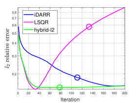


Figure 6 shows the reconstructed images computed by iDARR, LSQR, and the hybrid-l2 methods. Here the hybrid-l2 applies an -norm Tikhonov regularization to the projected problem obtained by LSQR, and it uses the stopping strategy in [12]. The best estimations of for iDARR or LSQR are solutions with minimizing . Their reconstructed solutions are obtained by using the L-curve method for early stopping.
Figure 7 (a)–(f) show the relative errors as the iteration number increases and the selection of the early stopping iterations by the L-curve method in the right two columns.
Notably, Figure 7 reveals that iDARR achieves more accurate reconstructed images than LSQR for both tests, despite appearing to the contrary in Figure fig:deblur. The LSQR appears prone to stopping late, resulting in lower-quality reconstructions than iDARR. In contrast, iDARR tends to stop earlier than ideal, before achieving the best quality. However, the hybrid-l2 method consistently produces accurate estimators with stable convergence, suggesting potential benefits in developing a hybrid iDARR approach to enhance stability.
The effectiveness of iDARR depends on the alignment of regularities between the convolution kernel and the image, as the DA-RKHS’s regularity is tied to the smoothness of the convolution kernel. With the PRblurspeckle featuring a smooth PSF, iDARR obtains a higher accuracy for the smoother Image-2 compared to Image-1, producing reconstructions with smooth edges. An avenue for future exploration involves adjusting the DA-RKHS’s smoothness to better align with the smoothness of the data.
6 Conclusion and Future Work
We have introduced iDARR, a scalable iterative data-adaptive RKHS regularization method, for solving ill-posed linear inverse problems. It searches for solutions in the subspaces where the true signal can be identified and achieves reliable early stopping via the DA-RKHS norm. A core innovation is a generalized Golub-Kahan bidiagonalization procedure that recursively computes orthonormal bases for a sequence of RKHS-restricted Krylov subspaces. Systematic numerical tests on the Fredholm integral equation show that iDARR outperforms the widely used iterative regularizations using the and norms, in the sense that it produces stable accurate solutions consistently converging when the noise level decays. Applications to 2D image de-blurring further show the iDARR outperforms the benchmark of LSQR with the norm.
Future Work: Hybrid Methods
The accuracy and stability of the regularized solution hinges on the choice of iteration number for early stopping. While the L-curve criterion is a commonly used tool for determining this number, it can sometimes lead to suboptimal results due to its reliance on identifying a corner in the discrete curve. Hybrid methods are well-recognized alternatives that help stabilize this semi-convergence issue, as referenced in [20, 8, 32]. One promising approach is to apply Tikhonov regularization to each iteration of the projected problem. The hyperparameter for this process can be determined using the weighted generalized cross-validation method (WGCV) as described in [8]. This approach is a focus of our upcoming research project.
References
- [1] Simon R Arridge, Marta M Betcke, and Lauri Harhanen. Iterated preconditioned LSQR method for inverse problems on unstructured grids. Inverse Probl., 30(7):075009, 2014.
- [2] Xianglan Bai, Guang-Xin Huang, Xiao-Jun Lei, Lothar Reichel, and Feng Yin. A novel modified TRSVD method for large-scale linear discrete ill-posed problems. Appl. Numer. Math., 164:72–88, 2021.
- [3] Frank Bauer, Sergei Pereverzev, and Lorenzo Rosasco. On regularization algorithms in learning theory. Journal of complexity, 23(1):52–72, 2007.
- [4] Chuan Bi, M. Yvonne Ou, Mustapha Bouhrara, and Richard G. Spencer. Span of regularization for solution of inverse problems with application to magnetic resonance relaxometry of the brain. Scientific Reports, 12(1):20194, 2022.
- [5] Åke Björck. A bidiagonalization algorithm for solving large and sparse ill-posed systems of linear equations. BIT Numer. Math., 28(3):659–670, 1988.
- [6] Noe Angelo Caruso and Paolo Novati. Convergence analysis of LSQR for compact operator equations. Linear Algebra and its Applications, 583:146–164, 2019.
- [7] Zhiming Chen, Wenlong Zhang, and Jun Zou. Stochastic convergence of regularized solutions and their finite element approximations to inverse source problems. SIAM Journal on Numerical Analysis, 60(2):751–780, 2022.
- [8] Julianne Chung, James G Nagy, and Dianne P O’Leary. A weighted-GCV method for Lanczos-hybrid regularization. Electr. Trans. Numer. Anal., 28(29):149–167, 2008.
- [9] Felipe Cucker and Ding Xuan Zhou. Learning theory: an approximation theory viewpoint, volume 24. Cambridge University Press, Cambridge, 2007.
- [10] Lars Eldén. A weighted pseudoinverse, generalized singular values, and constrained least squares problems. BIT Numer. Math., 22:487–502, 1982.
- [11] Heinz Werner Engl, Martin Hanke, and Andreas Neubauer. Regularization of inverse problems, volume 375. Springer Science & Business Media, 1996.
- [12] Silvia Gazzola, Per Christian Hansen, and James G Nagy. Ir tools: a matlab package of iterative regularization methods and large-scale test problems. Numerical Algorithms, 81(3):773–811, 2019.
- [13] Gene H. Golub and Charles F. Van Loan. Matrix Computations. The Johns Hopkins University Press, Baltimore, 4th edition, 2013.
- [14] Jacques Salomon Hadamard. Lectures on Cauchy’s problem in linear partial differential equations, volume 18. Yale University Press, 1923.
- [15] Per Christian Hansen. Rank-deficient and discrete ill-posed problems: numerical aspects of linear inversion. SIAM, 1998.
- [16] Per Christian Hansen. The L-curve and its use in the numerical treatment of inverse problems. In in Computational Inverse Problems in Electrocardiology, ed. P. Johnston, Advances in Computational Bioengineering, pages 119–142. WIT Press, 2000.
- [17] Guangxin Huang, Yuanyuan Liu, and Feng Yin. Tikhonov regularization with MTRSVD method for solving large-scale discrete ill-posed problems. J. Comput. Appl. Math., 405:113969, 2022.
- [18] Zhongxiao Jia and Yanfei Yang. A joint bidiagonalization based iterative algorithm for large scale general-form Tikhonov regularization. Appl. Numer. Math., 157:159–177, 2020.
- [19] Misha E. Kilmer, Per Christian Hansen, and Malena I. Espanol. A projection–based approach to general-form Tikhonov regularization. SIAM J. Sci. Comput., 29(1):315–330, 2007.
- [20] Misha E Kilmer and Dianne P O’Leary. Choosing regularization parameters in iterative methods for ill-posed problems. SIAM J. Matrix Anal. Appl., 22(4):1204–1221, 2001.
- [21] Jörg Lampe, Lothar Reichel, and Heinrich Voss. Large-scale Tikhonov regularization via reduction by orthogonal projection. Linear Algebra Appl., 436(8):2845–2865, 2012.
- [22] Quanjun Lang and Fei Lu. Small noise analysis for Tikhonov and RKHS regularizations. arXiv preprint arXiv:2305.11055, 2023.
- [23] Gongsheng Li and Zuhair Nashed. A modified Tikhonov regularization for linear operator equations. Numerical functional analysis and optimization, 26(4-5):543–563, 2005.
- [24] Haibo Li. A preconditioned Krylov subspace method for linear inverse problems with general-form Tikhonov regularization. arXiv:2308.06577v1, 2023.
- [25] Fei Lu, Qingci An, and Yue Yu. Nonparametric learning of kernels in nonlocal operators. Journal of Peridynamics and Nonlocal Modeling, pages 1–24, 2023.
- [26] Fei Lu, Quanjun Lang, and Qingci An. Data adaptive RKHS Tikhonov regularization for learning kernels in operators. Proceedings of Mathematical and Scientific Machine Learning, PMLR 190:158-172, 2022.
- [27] Fei Lu and Miao-Jung Yvonne Ou. An adaptive RKHS regularization for Fredholm integral equations. arXiv preprint arXiv:2303.13737, 2023.
- [28] M Zuhair Nashed and Grace Wahba. Generalized inverses in reproducing kernel spaces: an approach to regularization of linear operator equations. SIAM Journal on Mathematical Analysis, 5(6):974–987, 1974.
- [29] Dianne P O’Leary and John A Simmons. A bidiagonalization-regularization procedure for large scale discretizations of ill-posed problems. SIAM J. Sci. Statist. Comput., 2(4):474–489, 1981.
- [30] Christopher C Paige and Michael A Saunders. LSQR: An algorithm for sparse linear equations and sparse least squares. ACM Trans. Math. Software, 8:43–71, 1982.
- [31] Lothar Reichel, Fiorella Sgallari, and Qiang Ye. Tikhonov regularization based on generalized Krylov subspace methods. Appl. Numer. Math., 62(9):1215–1228, 2012.
- [32] R A Renaut, S Vatankhah, and V E Ardesta. Hybrid and iteratively reweighted regularization by unbiased predictive risk and weighted GCV for projected systems. SIAM J. Sci. Statist. Comput., 39(2):B221–B243, 2017.
- [33] Leonid I Rudin, Stanley Osher, and Emad Fatemi. Nonlinear total variation based noise removal algorithms. Physica D: nonlinear phenomena, 60(1-4):259–268, 1992.
- [34] Robert Tibshirani. Regression shrinkage and selection via the Lasso. Journal of the Royal Statistical Society: Series B (Methodological), 58(1):267–288, 1996.
- [35] Andrei Nikolajevits Tikhonov. Solution of incorrectly formulated problems and the regularization method. Soviet Math., 4:1035–1038, 1963.
- [36] Grace Wahba. Convergence rates of certain approximate solutions to fredholm integral equations of the first kind. Journal of Approximation Theory, 7(2):167–185, 1973.
- [37] Grace Wahba. Practical approximate solutions to linear operator equations when the data are noisy. SIAM journal on numerical analysis, 14(4):651–667, 1977.
- [38] Yimin Wei, Pengpeng Xie, and Liping Zhang. Tikhonov regularization and randomized GSVD. SIAM J. Matrix Anal. Appl., 37(2):649–675, 2016.
- [39] Hua Xiang and Jun Zou. Regularization with randomized svd for large-scale discrete inverse problems. Inverse Problems, 29(8):085008, 2013.
- [40] Hua Xiang and Jun Zou. Randomized algorithms for large-scale inverse problems with general Tikhonov regularizations. Inverse Probl., 31(8):085008, 2015.
- [41] Ye Zhang and Chuchu Chen. Stochastic asymptotical regularization for linear inverse problems. Inverse Problems, 39(1):015007, 2022.