Scalable Distributed Algorithms for Size-Constrained Submodular Maximization in the MapReduce and Adaptive Complexity Models
Abstract
Distributed maximization of a submodular function in the MapReduce (MR) model has received much attention, culminating in two frameworks that allow a centralized algorithm to be run in the MR setting without loss of approximation, as long as the centralized algorithm satisfies a certain consistency property – which had previously only been known to be satisfied by the standard greedy and continous greedy algorithms. A separate line of work has studied parallelizability of submodular maximization in the adaptive complexity model, where each thread may have access to the entire ground set. For the size-constrained maximization of a monotone and submodular function, we show that several sublinearly adaptive (highly parallelizable) algorithms satisfy the consistency property required to work in the MR setting, which yields practical, parallelizable and distributed algorithms. Separately, we develop the first distributed algorithm with linear query complexity for this problem. Finally, we provide a method to increase the maximum cardinality constraint for MR algorithms at the cost of additional MR rounds.
1 Introduction
Submodular maximization has become an important problem in data mining and machine learning with real world applications ranging from video summarization (Mirzasoleiman et al., 2018) and mini-batch selection (Joseph et al., 2019) to more complex tasks such as active learning (Rangwani et al., 2021) and federated learning (Balakrishnan et al., 2022). In this work, we study the size-constrained maximization of a monotone, submodular function (SMCC), formally defined in Section 1.3. Because of the ubiquity of problems requiring the optimization of a submodular function, a vast literature on submodular optimization exists; we refer the reader to the surveys (Liu et al., 2020; Liu, 2020).
| Reference | Ratio | MR Rounds | Adaptivity () | Queries () | |
| RG | |||||
| PAlg | |||||
| DDist | |||||
| BCG | |||||
| PG | |||||
| TG | |||||
| R-DASH (Alg. 4) | |||||
| G-DASH (Alg. 5) | |||||
| T-DASH (Alg. 10) | |||||
| L-Dist (Alg. 7) |
A foundational result of Nemhauser et al. (1978) shows that a simple greedy algorithm (Greedy, pseudocode in Appendix H) achieves the optimal approximation ratio for SMCC of in the value query model, in which the submodular function is available to the algorithm as an oracle that returns when queried with set . However, because of the modern revolution in data (Mao et al., 2021; Ettinger et al., 2021), there is a need for more scalable algorithms. Specifically, the standard greedy algorithm is a centralized algorithm that needs access to the whole dataset, makes many adaptive rounds (defined below) of queries to the submodular function, and has quadratic total query complexity in the worst case.
Distributed Algorithms for SMCC. Massive data sets are often too large to fit on a single machine and are distributed over a cluster of many machines. In this context, there has been a line of work developing algorithms for SMCC in the MapReduce model, defined formally in Section 1.3 (see Table 1 and the Related Work section below). Of these, PAlg (Barbosa et al., 2015) is a general framework that allows a centralized algorithm Alg to be converted to the MapReduce distributed setting with nearly the same theoretical approximation ratio, as long as Alg satisfies a technical, randomized consistency property (RCP), defined in Section 1.3.
In addition, DistributedDistorted (Kazemi et al., 2019), is also a general framework that can adapt any Alg satisfying RCP, as we show111In Kazemi et al. (2019), an instantiated version of DistributedDistorted with a distorted greedy algorithm is analyzed. in Section 4.2. However, to the best of our knowledge, the only centralized algorithms to satisfy this property are the Greedy Nemhauser et al. (1978) and the continuous greedy algorithm of Calinescu et al. (2007).
Parallelizable Algorithms for SMCC. A separate line of works, initiated by Balkanski and Singer (2018) has taken an orthogonal approach to scaling up the standard greedy algorithm: parallelizable algorithms for SMCC as measured by the adaptive complexity of the algorithm, formally defined in Section 1.3. In this model, each thread may have access to the entire ground set and hence these algorithms do not apply in a distributed setting. Altogether, these algorithms have exponentially improved the adaptivity of standard greedy from to while obtaining the nearly the same approximation ratio Fahrbach et al. (2019a); Balkanski et al. (2019); Ene and Nguyen (2019); Chekuri and Quanrud (2019). Recently, highly practical sublinearly adaptive algorithms have been developed without compromising theoretical guarantees Breuer et al. (2020); Chen et al. (2021). However, none of these algorithms have been shown to satisfy the RCP.
Combining Parallelizability and Distributed Settings. In this work, we study parallelizable, distributed algorithms for SMCC; each node of the distributed cluster likely has many processors, so we seek to take advantage of this situation by parallelizing the algorithm within each machine in the cluster. In the existing MapReduce algorithms, the number of processors could be set to the number of processors available to ensure the usage of all available resources – this would consider each processor as a separate machine in the cluster. However, there are a number of disadvantages to this approach: 1) A large number of machines severely restricts the size of the cardinality constraint – since, in all of the MapReduce algorithms, a set of size must be stored on a single machine; therefore, we must have . For example, with , implies that , for some . However, if each machine has 8 processor cores, the number of machines can be set to 32 (and then parallelized on each machine), which enables the use of 256 processors with . As the number of cores and processors per physical machine continues to grow, large practical benefits can be obtained by a parallelized and distributed algorithm. 2) Modern CPU architectures have many cores that all share a common memory, and it is inefficient to view communication between these cores to be as expensive as communication between separate machines in a cluster.
In addition to the MapReduce and adaptive complexity models, the total query complexity of the algorithm to the submodular oracle is also relevant to the scalability of the algorithm. Frequently, evaluation of the submodular function is expensive, so the time spent answering oracle queries dominates the other parts of the computation. Therefore, the following questions are posed: Q1: Is it possible to design constant-factor approximation distributed algorithms with 1) constant number of MapReduce rounds; 2) sublinear adaptive complexity (highly-parallelizable); and 3) nearly linear total query complexity? Q2: Can we design practical distributed algorithms that also meet these three criteria?
1.1 Contributions
In overview, the contributions of the paper are: 1) an exponential improvement in adaptivity (from to for an algorithm with a constant number of MR rounds; 2) the first linear-time, constant-factor algorithm with constant MR rounds; 3) a way to increase the size constraint limitation at the cost of additional MR rounds; and 4) an empirical evaluation on a cluster of 64 machines that demonstrates an order of magnitude improvement in runtime is obtained by combining the MR and adaptive complexity models.
To develop MR algorithms with sublinear adaptivity, we first modify and analyze the low-adaptive algorithm ThreshSeqMod from Chen et al. (2021) and show that our modification satisfies the RCP (Section 2). Next, ThreshSeqMod is used to create a low-adaptive greedy procedure LAG; LAG then satisfies the RCP, so can be used within PAlg Barbosa et al. (2016) to yield a approximation in MR rounds, with adaptivity . We show in Section 4.2 that DistributedDistorted Kazemi et al. (2021) also works with any Alg satisfying RCP, which yields an improvement in the number of MR rounds to achieve the same ratio. The resulting algorithm we term G-DASH (Section 4), which achieves ratio with adaptivity and MR rounds.
Although G-DASH achieves nearly the optimal ratio in constant MR rounds and sublinear adaptivity, the number of MR rounds is high. To obtain truly practical algorithms, we develop constant-factor algorithms with 2 MR rounds: R-DASH and T-DASH with and adaptivity, respectively, and with approximation ratios of ( 0.316) and . R-DASH is our most practical algorithm and may be regarded as a parallelized version of RandGreeDI Barbosa et al. (2015), the first MapReduce algorithm for SMCC and the state-of-the-art MR algorithm in terms of empirical performance. T-DASH is a novel algorithm that improves the theoretical properties of R-DASH at the cost of empirical performance (see Table 1 and Section 8). Notably, the adaptivity of T-DASH is which is close to the best known adaptivity for a constant factor algorithm of Chen et al. (2021), which has adaptivity of .
Although our MR algorithms are nearly linear time (within a polylogarithmic factor of linear), all of the existing MR algorithms are superlinear time, which raises the question of if an algorithm exists that has a linear query complexity and has constant MR rounds and constant approximation factor. We answer this question affirmatively by adapting a linear-time algorithm of Kuhnle (2021); Chen et al. (2021), and showing that our adaptation satisfies RCP (Section 3). Subsequently, we develop the first MR algorithm (L-Dist) with an overall linear query complexity.
Our next contribution is MED, a general plug-in framework for distributed algorithms, which increases the size of the maximum cardinality constraint at the cost of more MR rounds. As discussed above, the maximum value of any prior MR algorithm for SMCC is , where is the number of machines; MED increases this to . We also show that under certain assumptions on the objective function (which are satisfied by all of the empirical applications evaluated in Section 8), MED can be run with , which removes any cardinality restrictions. When used in conjunction with a -approximation MR algorithm, MED provides an ()-approximate solution.
Finally, an extensive empirical evaluation of our algorithms and the current state-of-the-art on a 64-machine cluster with 32 cores each and data instances ranging up to 5 million nodes show that R-DASH is orders of magnitude faster than state-of-the-art MR algorithms and demonstrates an exponential improvement in scaling with larger . Moreover, we show that MR algorithms slow down with increasing number of machines past a certain point, even if enough memory is available, which further motivates distributing a parallelizable algorithm over smaller number of machines. This observation also serves as a motivation for the development of the MED+Alg framework. In our evaluation, we found that the MED+Alg framework delivers solutions significantly faster than the Alg for large constraints, showcasing its superior performance and efficiency.
A previous version of this work was published in a conference Dey et al. (2023). In that version, RCP was claimed to be shown for the ThresholdSeq algorithm of Chen et al. (2021). Unfortunately, RCP does not hold for this algorithm. In this version, we provide a modified version of the ThresholdSeq algorithm of Chen et al. (2021), for which we show RCP. Additionally, in this version, we introduce the first linear time MR algorithm, LinearTime-Distributed (L-Dist). Finally, in our empirical evaluation, we expand upon the conference version by conducting two additional experiments using a larger cluster comprising 64 machines. These additional experiments aim to evaluate the performance of L-Dist and investigate the effectiveness of MED in handling increasing cardinality constraints, respectively.
1.2 Organization
The rest of this paper is organized as follows. In Section 2, we present the low-adaptive procedures and show they satisfy the RCP. In Section 3, we analyze an algorithm with linear query complexity and show it satisfies the RCP. In Section 4, we show how to use algorithms satisfying the RCP to obtain MR algorithms. In Section 5, we improve the theoretical properties of our 2-round MR algorithm. In Section 6, we detail the linear-time MR algorithm. In Section 7, we show how to increase the supported constraint size by adding additional MR rounds. In Section 8, we conduct our empirical evaluation.
1.3 Preliminaries
A submodular set function captures the diminishing gain property of adding an element to a set that decreases with increase in size of the set. Formally, let be a finite set of size . A non-negative set function is submodular iff for all sets and , . The submodular function is monotone if for all . We use to denote the marginal game of element to set : . In this paper, we study the following optimization problem for submodular optimization under cardinality constraint (SMCC):
| (1) |
MapReduce Model. The MapReduce (MR) model is a formalization of distributed computation into MapReduce rounds of communication between machines. A dataset of size is distributed on machines, each with memory to hold at most elements of the ground set. The total memory of the machines is constrained to be . After each round of computation, a machine may send amount of data to other machines. We assume for some constant .
Next, we formally define the RCP needed to use the two frameworks to convert a centralized algorithm to the MR setting, as discussed previously.
Property 1 (Randomized Consistency Property of Barbosa et al. (2016)).
Let be a fixed sequence of random bits; and Alg be a randomized algorithm with randomness determined by . Suppose returns a pair of sets, , where is the feasible solution and is a set providing additional information. Let and be two disjoint subsets of , and that for each , . Also, suppose that terminates successfully. Then terminates successfully and .
Adaptive Complexity. The adaptive complexity of an algorithm is the minimum number of sequential adaptive rounds of at most polynomially many queries, in which the queries to the submodular function can be arranged, such that the queries in each round only depend on the results of queries in previous rounds.
1.4 Related Work
MapReduce Algorithms. Addressing the coverage maximization problem (a special case of SMCC), Chierichetti et al. (2010) proposed an approximation algorithm achieving a ratio of , with polylogarithmic MapReduce (MR) rounds. This was later enhanced by Blelloch et al. (2012), who reduced the number of rounds to . Kumar et al. (2013) contributed further advancements with a algorithm, significantly reducing the number of MR rounds to logarithmic levels. Additionally, they introduced a approximation algorithm that operates within MR rounds, albeit with a logarithmic increase in communication complexity.
For SMCC, Mirzasoleiman et al. (2013) introduced the two-round distributed greedy algorithm (GreedI), demonstrating its efficacy through empirical studies across various machine learning applications. However, its worst-case approximation guarantee is . Subsequent advancements led to the development of constant-factor algorithms by Barbosa et al. (2015). Barbosa et al. (2015) notably introduced randomization into the distributed greedy algorithm GreedI, resulting in the RandGreeDI algorithm. This algorithm achieves a approximation ratio with two MR rounds and queries. Mirrokni and Zadimoghaddam (2015) also introduced an algorithm with two MR rounds, where the first round finded randomized composable core-sets and the second round applied a tie-breaking rule. This algorithm improve the approximation ratio from to . Later on, Barbosa et al. (2016) proposed a round algorithm with the optimal approximation ratio without data duplication. Then, Kazemi et al. (2021) improved its space and communication complexity by a factor of with the same approximation ratio. Another two-round algorithm, proposed by Liu and Vondrak (2019), achieved an approximation ratio, but requires data duplication with four times more elements distributed to each machine in the first round. As a result, distributed setups have a more rigid memory restriction when running this algorithm.
Parallelizable Algorithms. A separate line of works consider the parallelizability of the algorithm, as measured by its adaptive complexity. Balkanski and Singer (2018) introduced the first -adaptive algorithm, achieving a approximation ratio with query complexity for SMC Then, Balkanski et al. (2019) enhanced the approximation ratio to with query complexity while maintaining the same sublinear adaptivity. In the meantime, Ene and Nguyen (2019), Chekuri and Quanrud (2019), and Fahrbach et al. (2019a) achieved the same approximation ratio and adaptivity but with improved query complexities: for Ene and Nguyen (2019), for Chekuri and Quanrud (2019), and for Fahrbach et al. (2019a). Recently, highly practical sublinearly adaptive algorithms have been developed without compromising on the approximation ratio. FAST, introduced by Breuer et al. (2020), operates with adaptive rounds and queries, while LS+PGB, proposed by Chen et al. (2021), runs with adaptive rounds and queries. However, none of these algorithms have been shown to satisfy the RCP.
Fast (Low Query Complexity) Algorithms. Since a query to the oracle for the submodular function is typically an expensive operation, the total query complexity of an algorithm is highly relevant to its scalability. The work by Badanidiyuru and Vondrak (2014) reduced the query complexity of the standard greedy algorithm from to , while nearly maintaining the ratio of . Subsequently, Mirzasoleiman et al. (2015) utilized random sampling on the ground set to achieve the same approximation ratio in expectation with optimal query complexity. Afterwards, Kuhnle (2021) obtained a deterministic algorithm that achieves ratio in exactly queries, and the first deterministic algorithm with query complexity and approximation ratio. Since our goal is to develop practical algorithms in this work, we develop paralellizable and distributed algorithms with nearly linear query complexity (i.e. within a polylogarithmic factor of linear). Further, we develop the first linear-time algorithm with constant number of MR rounds, although it doesn’t parallelize well.
Non-monotone Algorithms. If the submodular function is no longer assumed to be monotone, the SMCC problem becomes more difficult. Here, we highlight a few works in each of the categories of distributed, parallelizable, and query efficient. Lee et al. (2009) provided the first constant-factor approximation algorithm with an approximation ratio of and a query complexity of . Building upon that, Gupta et al. (2010) reduced the query complexity to by replacing the local search procedure with a greedy approach that resulted in a slightly worse approximation ratio. Subsequently, Buchbinder et al. (2014) incorporated randomness to achieve an expected approximation ratio with query complexity. Furthermore, Buchbinder et al. (2017) improved it to query complexity while maintaining the same approximation ratio in expectation. For parallelizable algorithms in the adaptive complexity model, Ene and Nguyen (2020) achieved the current best approximation ratio with adaptivity and queries to the continuous oracle (a continuous relaxation of the original value oracle). Later, Chen and Kuhnle (2024) achieved the current best sublinear adaptivity and nearly linear query complexity with a approximation ratio. In terms of distributed algorithms in the MapReduce model, RandGreeDI proposed by Barbosa et al. (2015) achieved a approximation ratio within MR rounds and query complexity. Simulaneously, Mirrokni and Zadimoghaddam (2015) also presented a -round algorithm with a approximation ratio and query complexity. Afterwards, Barbosa et al. (2016) proposed a -round continuous algorithm with a approximation ratio.
2 Low-Adaptive Algorithms That Satisfy the RCP
In this section, we analyze two low-adaptive procedures, ThreshSeqMod (Alg. 1), LAG (Alg. 2), variants of low-adaptive procedures proposed in Chen et al. (2021). This analysis enables their use in the distributed, MapReduce setting. For convenience, we regard the randomness of the algorithms to be determined by a sequence of random bits , which is an input to each algorithm.
Observe that the randomness of both of ThreshSeqMod and LAG only comes from the random permutations of on Line 8 of ThreshSeqMod, since LAG employs ThreshSeqMod as a subroutine. Consider an equivalent version of these algorithms in which the entire ground set is permuted randomly, from which the permutation of is extracted. That is, if is the permutation of , the permutation of is given by iff , for . Then, the random vector specifies a sequence of permutations of : , which completely determines the behavior of both algorithms.
2.1 Low-Adaptive Threshold (ThreshSeqMod) Algorithm
This section presents the analysis of the low-adaptive threshold algorithm, ThreshSeqMod (Alg. 1; a variant of ThresholdSeq from Chen et al. (2021)). In ThreshSeqMod, the randomness is explicitly dependent on a random vector . This modification ensures the consistency property in the distributed setting. Besides the addition of randomness q, ThreshSeqMod employs an alternative strategy of prefix selection within the for loop. Instead of identifying the failure point (the average marginal gain is under the threshold) after the final success point (the average marginal gain is above the threshold) in Chen et al. (2021), ThreshSeqMod determines the first failure point. This adjustment not only addresses the consistency problem but also preserves the theoretical guarantees below.
Theorem 1.
Suppose ThreshSeqMod is run with input . Then, the algorithm has adaptive complexity and outputs , where is the solution set with and provides additional information with . The following properties hold: 1) The algorithm succeeds with probability at least . 2) There are oracle queries in expectation. 3) It holds that . 4) If , then for all .
2.1.1 Analysis of Consistency
Lemma 1.
ThreshSeqMod satisfies the randomized consistency property (Property 1).
Proof.
Consider that the algorithm runs for all iterations of the outer for loop; if the algorithm would have returned at iteration , the values and , for keep their values from when the algorithm would have returned. The proof relies upon the fact that every call to uses same sequences of permutations of : . We refer to iterations of the outer for loop on Line 4 of Alg. 1 simply as iterations. Since randomness only happens with the random permutation of at each iteration in Alg. 1, the randomness of is determined by , which satisfies the hypothesis of Property 1.
For the two sets returned by , represents the feasible solution, and is the set that provides additional information. We consider the runs of (1) , (2) , and (3) together. Variables of (1) are given the notation defined in the pseudocode; variables of (2) are given the superscript ; and variables of (3) are given the superscript ′. Suppose for each , . The lemma holds if and terminates successfully.
Let be the statement for iteration of the outer for loop on Line 4 that
-
(i)
, and
-
(ii)
for all , , , and
-
(iii)
, and
-
(iv)
for all , .
If is true, and and terminate at the same iteration, implying that also terminates successfully, then the lemma holds immediately. In the following, we prove these two statements by induction.
For , it is clear that , and for all . Therefore, is true. Next, suppose that is true. We show that is also true, and if terminates at iteration , also terminates at iteration .
Firstly, we show that (iii) and (iv) of hold. Since holds, it indicates that for any by (i) and (ii) of . So, (iii) and (iv) of clearly hold since the sets involved in updating , on Line 5 are equal (after is removed).
Secondly, we prove that (i) and (ii) of hold and that if terminates at iteration , also terminates at iteration .
If terminates at iteration because , then the other two runs of ThreshSeqMod also terminate at iteration , since by (i) and (ii) of . Moreover, (i) and (ii) of are true since , , , , and do not update.
If terminates at iteration because , then by (iii) and (iv) of , it holds that for all . Thus, must be empty; otherwise, and will be added to at iteration which contradicts the fact that . Therefore, has been filtered out before iteration or will be filtered out at iteration in both and since the sets and involved in updating and are the same. Consequently, is also an empty set and terminates at iteration . Futhermore, (i) and (ii) of are true since , , , , and do not update.

Finally, consider the case that does not terminate at iteration , where and . By (iii) and (iv), it holds that , for any . Let be the first element appeared in the sequence of , be the index of in the order of the permutation of . If such does not exist (i.e. , for any ), let . Fig. 1 depicts the relationship between three sequences , and . Let , , be sets added to , , at iteration respectively. Since and are subsets of the same random permutation of , and , is also the index of in . Also, it holds that
| (2) |
Since , it holds that , which indicates that . By the definition of on Line 16,
Follows from Equality 2, and , it holds that
Therefore, , and even further . So, Property (i) and (ii) hold.
∎
2.1.2 Analysis of Guarantees
There are three adjustments in ThreshSeqMod compared with ThresholdSeq in Chen et al. (2021) altogether. First, we made the randomness explicit allowing us to still consider each permutation on Line 8 as a random step. Therefore, the analysis of the theoretical guarantees is not influenced by adopting the randomness . Second, the prefix selection step is changed from identifying the failure point after the final success point to identifying the initial failure point. Note that, this change is necessary for the algorithm to satisfy RCP (Property1). However, by making this change, fewer elements could be filtered out at the next iteration. Fortunately, we are still able to filter out a constant fraction of the candidate set. Third, the algorithm returns one more set that provides extra information. Since the additional set does not affect the functioning of the algorithm, it does not influence the theoretical guarantees. In the following, we will provide the detailed analysis for the theoretical guarantees.
As demonstrated by Lemma 2 below, an increase in the number of selected elements results in a corresponding increase in the number of filtered elements. Consequently, there exists a point, say , such that a given constant fraction of can be filtered out if we are adding more than elements. The proof of this lemma is quite similar to the proof of Lemma 12 in Chen et al. (2021) which can be found in Appendix C.
Lemma 2.
At an iteration , let after Line 5. It holds that , and .
Although we use a smaller prefix based on Line 16 and 18 compared to ThresholdSeq, it is still possible that with probability at least , a constant fraction of will be filtered out at the beginning of iteration , or the algorithm terminates with ; given as Lemma 3 in the following. Intuitively, if there are enough such iterations, ThreshSeqMod will succeed. Also, the calculation of query complexity comes from Lemma 3 directly. Since the analyses of success probability, adaptivity and query complexity simply follows the analysis in Chen et al. (2021), we provide these analyses in Appendix C. Next, we prove that Lemma 3 always holds.
Lemma 3.
Proof.
By the definition of in Lemma 2, will be filtered out from at the next iteration. Equivalently, . After Line 8 at iteration , by Lemma 2, there exists a such that . We say an iteration succeeds, if . In this case, it holds that either , or . In other words, iteration succeeds if there does not exist such that by the selection of on Line 18. Instead of directly calculating the success probability, we consider the failure probability. Define an element bad if , and good otherwise. Consider the random permutation of as a sequence of dependent Bernoulli trials, with success if the element is bad and failure otherwise. When , the probability of is bad is less than . If , there are at least bad elements in . Let be a sequence of independent and identically distributed Bernoulli trials, each with success probability . Next, we consider the following sequence of dependent Bernoulli trials , where when , and otherwise. Define if there are at least bad elements in . Then, for any , it holds that . In the following, we bound the probability that there are more than -fraction s in for any ,
| (Lemma 9) | ||||
| (Markov’s Inequality, Lemma 10) | ||||
| () |
Subsequently, the probability of failure at iteration is calculated below,
∎
2.2 Low-Adaptive Greedy (LAG) Algorithm
Another building block for our distributed algorithms is a simple, low-adaptive greedy algorithm LAG (Alg. 2). This algorithm is an instantiation of the ParallelGreedyBoost framework of Chen et al. (2021), and it relies heavily on the low-adaptive procedure ThreshSeqMod (Alg. 1).
Guarantees. Following the analysis of Theorem 3 in Chen et al. (2021), LAG achieves ratio in adaptive rounds and total queries with probability at least . Setting and , LAG has adaptive complexity of and a query complexity of
Lemma 4.
LAG satisfies the randomized consistency property (Property 1).
Proof of Lemma 4.
Observe that the only randomness in LAG is from the calls to ThreshSeqMod. Since succeeds, every call to ThreshSeqMod must succeed as well. Moreover, considering that is used to permute the underlying ground set , changing the set argument of LAG does not change the sequence received by each call to ThreshSeqMod. Order the calls to ThreshSeqMod: , , …, . Since , it holds that , for each and each . If is equivalent to (as shown in Claim 1 in the following), then by application of Lemma 1, terminates successfully and for each . Therefore, and the former call terminates successfully. ∎
Next, we provide Claim 1 and its analysis below.
Claim 1.
Let be a fixed sequence of random bits, , and . Then, if and only if .
Proof.
It is obvious that if , then . In the following, we prove the reverse statement.
Following the analysis of RCP for ThreshSeqMod in Section 2.1.1, we consider the runs of (1) , and (2) . Variables of (1) are given the notation defined in the pseudocode; variables of (2) are given the superscript . We analyze the following statement for each iteration of the outer for loop on Line 4 in Alg. 1.
-
(i)
for all , , , and
-
(ii)
for all , .
Since , then for each . Thus, the analysis in Section 2.1.1 also holds in this case. According to the inductive method, we are able to prove that is true for each which indicates . ∎
3 Consistent Linear Time (Linear-TimeCardinality) Algorithm
In this section, we present the analysis of Linear-TimeCardinality (Alg. 3, LTC), a consistent linear time algorithm which is an extension of the highly adaptive linear-time algorithm (Alg. 3) in Chen et al. (2021). Notably, to ensure consistency within a distributed setting and bound the solution size, LTC incorporates the randomness q, and initializes the solution set with the maximum singleton. The algorithm facilitates the creation of linear-time MapReduce algorithms, enhancing overall computational efficiency beyond the capabilities of current state-of-the-art superlinear algorithms.
Theorem 2.
Let be an instance of SM. The algorithm Linear-TimeCardinality outputs such that the following properties hold: 1) There are oracle queries and adaptive rounds. 2) Let be the last elements in . It holds that , where is an optimal solution to the instance . 3) The size of is limited to .
3.1 Analysis of Consistency
The highly adaptive linear-time algorithm (Alg. 3) outlined in Chen et al. (2021) commences with an empty set and adds elements to it iff. . Without introducing any randomness, this algorithm can be deterministic only if the order of the ground set is fixed. Additionally, to limit the solution size, we initialize the solution set with the maximum singleton, a choice that also impacts the algorithm’s consistency. However, by selecting the first element that maximizes the objective value, the algorithm can maintain its consistency. In the following, we provide the analysis of randomized consistency property of LTC.
Lemma 5.
LTC satisfies the randomized consistency property (Property 1).
Proof.
Consider the runs of (1) , (2) , and (3) . With the same sequence of random bits q, after the random permutation, , and are the subsets of the same sequence. For any , let be the index of . Then, are the elements before (including ). Define be the intermediate solution of (1) after we consider element . If , define . Similarly, define and be the intermediate solution of (2) and (3). If , for any and , . Next, we prove the above statement holds.
For any , since , it holds that either , or , and , where is the first element in . Therefore, is also the first element in . Furthermore, it holds that .
Suppose that . If or , naturally, . If , immediately. Since , it holds that and . So, . Then, . Thus, . ∎
3.2 Analysis of Guarantees
Query Complexity and Adaptivity. Alg. 3 queries on Line 4 and 6, where there are oracle queries on Line 4 and 1 oracle query for each element received on Line 6. Therefore, the query complexity and the adaptivity are both .
Solution Size. Given that is a monotone function, it holds that . Furthermore, since , the submodularity property implies that . Each element added to contributes to an increase in the solution value by a factor of . Therefore,
| () |
Objective Value. For any , let be the intermediate solution before we process . It holds that for any . Then,
where Inequality (1) follows from monotonicity and submodularity, Inequality (2) follows from submodularity.
For any , it holds that . Then,
where Inequalities (1) and (2) follow from submodularity.
4 Low-Adaptive Algorithms with Constant MR Rounds (Greedy-DASH and Randomized-DASH)
Once we have the randomized consistency property of LAG, we can almost immediately use it to obtain parallelizable MapReduce algorithms.
4.1 Randomized-DASH
R-DASH (Alg. 4) is a two MR-rounds algorithm obtained by plugging LAG into the RandGreeDI algorithm of Mirzasoleiman et al. (2013); Barbosa et al. (2015). R-DASH runs in two MapReduce rounds, adaptive rounds, and guarantees the ratio ( 0.316).
Description. The ground set is initially distributed at random by R-DASH across all machines . In its first MR round, R-DASH runs LAG on every machine to obtain in adaptive rounds. The solutions from every machine are then returned to the primary machine, where LAG selects the output solution that guarantees approximation in adaptive rounds as stated in Corollary 1. First, we provide Theorem 3 and its analysis by plugging any randomized algorithm Alg which follows RCP (Property 1) into the framework of RandGreeDI. The proof is a minor modification of the proof of Barbosa et al. (2015) to incorporate randomized consistency. Then, we can get Corollary 1 for R-DASH immediately.
Theorem 3.
Let be an instance of SM where . Alg is a randomized algorithm which satisfies the Randomized Consistency Property with approximation ratio, query complexity, and adaptivity. By replacing LAG with Alg, R-DASH returns set with two MR rounds, adaptive rounds, total queries, communication complexity such that
Proof.
Query Complexity and Adaptivity. R-DASH runs with two MR rounds. In the first MR round, Alg is invoked times in parallel, each with a ground set size of . So, during the first MR round, the number of queries is and the number of adaptive rounds is . Then, the second MR round calls Alg once, handling at most elements. Consequently, the total number of queries of R-DASH is , and the total number of adaptive rounds is .
Approximation Ratio. Let R-DASH be run with input . Since , . By an application of Chernoff’s bound to show that the size is concentrated.
Let denote the random distribution over subsets of where each element is included independently with probability . For , let
Consider and on machine . Let . Since Alg follows the Randomized Consistency Property, . Therefore, . Next, let , where . It holds that . Let ; is assigned to on some machine . It holds that,
Therefore,
| (3) |
Corollary 1.
Let be an instance of SM where . R-DASH returns set with two MR rounds, adaptive rounds, total queries, communication complexity, and probability at least such that
4.2 Greedy-DASH
Next, we obtain the nearly the optimal ratio by applying LAG and randomized consistency to DistributedDistorted proposed by Kazemi et al. (2021). DistributedDistorted is a distributed algorithm for regularized submodular maximization that relies upon (a distorted version of) the standard greedy algorithm. For SMCC, the distorted greedy algorithm reduces to the standard greedy algorithm Greedy. In the following, we show that any algorithm that satisfies randomized consistency can be used in place of Greedy as stated in Theorem 4. By introducing LAG into DistributedDistorted, G-DASH achieves the near optimal () expected ratio in MapReduce rounds, adaptive rounds, and total queries. We also generalize this to any algorithm that satisfies randomized consistency.
The Framework of Kazemi et al. (2021). DistributedDistorted has MR rounds where each round works as follows: First, it distributes the ground set into machines uniformly at random. Then, each machine runs Greedy (when modular term ) on the data that combines the elements distributed before each round and the elements forwarded from the previous rounds to get the solution . At the end, the final solution, which is the best among and all the previous solutions, is returned. To improve the adaptive rounds of DistributedDistorted, we replace standard greedy with LAG to get G-DASH.
Theorem 4.
Let be an instance of SM where . Alg is a randomized algorithm which satisfies the Randomized Consistency Property with approximation ratio, query complexity, and adaptivity. By replacing LAG with Alg, G-DASH returns set with MR rounds and adaptive rounds, total queries, communication complexity such that,
Proof.
Query Complexity and Adaptivity. G-DASH operates with MR rounds, where each MR round calls Alg times in parallel. As each call of Alg works on the ground set with a size of at most , the total number of queries for G-DASH is , and the total number of adaptive rounds is .
Approximation ratio. Let G-DASH be run with input . Similar to the analysis of Theorem 3, The size of is concentrated. Let be the optimal solution. For any , define that,
Then we provide the following lemma.
Lemma 6.
For any and , .
Proof.
∎
The rest of the proof bounds in the following two ways.
First, let , and . Since Alg follows the Randomized Consistency Property, it holds that , and . So, for any ,
Therefore,
| (4) |
Corollary 2.
Let be an instance of SM where . G-DASH returns set with MR round and adaptive rounds, total queries, communication complexity, and probability at least such that,
5 Threshold-DASH: Two MR-Rounds Algorithm with Improved Theoretical Properties
In this section, we present a novel )-approximate, two MR-rounds algorithm Threshold-DASH (T-DASH) that achieves nearly optimal adaptivity in total time complexity.
Description. The T-DASH algorithm (Alg. 6) is a two MR-rounds algorithm that runs ThreshSeqMod concurrently on every machine with a specified threshold value of . The primary machine then builds up its solution by adding elements with ThreshSeqMod from the pool of solutions returned by the other machines. Notice that there is a small amount of data duplication as elements of the ground set are not randomly partitioned in the same way as in the other algorithms. This version of the algorithm requires to know the OPT value; in Appendix E we show how to remove this assumption. In Appendix I, we further discuss the similar two MR round algorithm of Liu and Vondrak (2019), that provides an improved -approximation but requires four times the data duplication of T-DASH.
Theorem 5.
Let be an instance of SM where . T-DASH knowing OPT returns set with two MR rounds, adaptive rounds, total queries, communication complexity, and probability at least such that
Proof.
Query Complexity and Adaptivity. T-DASH runs with two MR rounds, where the first MR round invokes ThreshSeqMod times in parallel, and the second MR round invokes ThreshSeqMod once. By Theorem 1, each call of ThreshSeqMod with a ground set of size at most queries within adaptive rounds. The total number of queries is , and the total number of adaptive rounds is .
Approximation Ratio. In Algorithm 6, there are independent calls of ThreshSeqMod. With , the success probability of each call of ThreshSeqMod is larger than . Thus, Algorithm 6 succeeds with probability larger than . For the remainder of the analysis, we condition on the event that all calls to ThreshSeqMod succeed.
In the case that , by Theorem 1 in Section 2.1 and , it holds that Otherwise, we consider the case that in the following. Let be the pair of sets returned by . For any , let
Let , . By Randomized Consistency Property, it holds that . For any , is not selected in . Since, , by Property (4) in Theorem 1, Also, for any , is not selected in . Similarly, Then, we can get,
| (6) |
Next, we provide the following lemma to complete the rest of the proof.
Lemma 7.
For any , it holds that .
6 LinearTime-Distributed (L-Dist)
In this section, we introduce L-Dist, the first linear time MapReduce algorithm with constant approximation. We derive L-Dist from R-DASH by incorporating the analysis of LTC (Alg. 3), an algorithm with query complexity, into the distributed setting. This integration allows L-Dist to operate within two MapReduce rounds, demonstrating an adaptive complexity of and a query complexity of . Also, as stated in Theorem 6, it guarantees an approximation ratio of . Additionally, we improve the objective value by implementing ThresholdGreedy (Alg. 9 in Appendix D) on the set returned at the second MapReduce round. The integration of LTC into LinearTime-Distributed provides enhanced capabilities and improves the efficiency of the overall algorithm.
Description: Initially, L-Dist involves randomly distributing the ground set across all machines . In the first MR round, LinearTime-Distributed applies LTC on each machine to obtain within query calls. The solutions from all machines are then returned to the primary machine, where LTC selects the output solution . By selecting the best last among all solutions, L-Dist ensures a -approximation. Besides returning the last elements of the solution which is an -approximation of , we employ ThresholdGreedy, a approximation algorithm, to boost the objective value. We provide the theoretical guarantees of L-Dist as Theorem 6. The proof involves a minor modification of the proof provided in Theorem 3.
Theorem 6.
Let be an instance of SM where . L-Dist returns a set with two MR rounds, adaptive rounds, total queries, communication complexity such that
6.1 Analysis of Query Complexity and Adaptivity
L-Dist runs with two MR rounds. In the first MR round, LTC is invoked times in parallel, each with queries and adaptive rounds by Theorem 2. So, during the first MR round, the number of queries is and the number of adaptive rounds is . Then, the second MR round calls LTC and ThresholdGreedy once respectively, handling at most elements. By Theorem 2 and 8, the number of queries is and the number of adaptive rounds is . Consequently, the total number of queries of L-Dist is , and the total number of adaptive rounds is .
6.2 Analysis of Approximation Ratio
Let L-Dist be executed with input . Since , it follows that the expected size of each subset satisfies . To ensure that the size is concentrated, we apply Chernoff’s bound. Let denote the random distribution over subsets of where each element is included independently with probability . Let be the following vector. For , let
Consider on machine . Let . By Lemma 5, . Therefore, by Theorem 2, it holds that . Next, let , where . Similarly, by Theorem 2, it holds that . Let ; is assigned to on some machine . It holds that,
6.3 Post-Processing
In this algorithm, we employ a simple post-processing procedure. Since is an approximation of with size , is also an approximation of the instance on the ground set . By running any linear time algorithm that has a better approximation ratio on , we are able to boost the objective value returned by the algorithm with the same theoretical guarantees. By Theorem 8, ThresholdGreedy achieves approximation in linear time with a guess on the optimal solution. Therefore, with input and , utilizing ThresholdGreedy can effectively enhance the objective value.
7 Towards Larger : A Memory-Efficient, Distributed Framework (MED)
In this section, we propose a general-purpose plug-in framework for distributed algorithms, MemoryEfficientDistributed (MED, Alg. 8). MED increases the largest possible constraint value from to in the value oracle model. Under some additional assumptions, we remove all restrictions on the constraint value.
As discussed in Section 1, the value is limited to a fraction of the machine memory for MapReduce algorithms: , since those algorithms need to merge a group of solutions and pass it to a single machine. MED works around this limitation as follows: MED can be thought of as a greedy algorithm that uses an approximate greedy selection through Alg. One machine manages the partial solutions , built up over iterations. In this way, each call to Alg is within the constraint restriction of Alg, i.e. , but a larger solution of up to size can be constructed.
The restriction on of MED of comes from passing the data of the current solution to the next round. Intuitively, if we can send some auxiliary information about the function instead of the elements selected, the value can be unrestricted.
Assumption 1.
Let be a set function with ground set of size . If for all , there exists a bitvector , such that the function can be computed from and , then satisfies Assumption 1.
We show in Appendix F that all four applications evaluated in Section 8 satisfy Assumption 1. As an example, consider MaxCover, which can be expressed as , where . Let , and . Then, , where the first term is given by and the second term is calculated by . Therefore, since , can be computed from and .
Theorem 7.
Let () be an instance of SMCC distributed over machines. For generic objectives, where the data of current solution need to be passed to the next round, ; for special objectives, where only one piece of compressed data need to be passed to the next round, . Let be the set returned by MED. Then , where is the expected approximation of Alg.
Proof.
Let be an optimal and be a partition of into pieces, each of size . Also is monotone SMCC since is monotone SMCC.
where Inequality (a) follows from is SMCC; Alg is -approximation. Unfix , it holds that
To analyze the memory requirements of MED, consider the following. To compute , the current solution need to be passed to each machine in for the next call of Alg. Suppose where . The size of data stored on any non-primary machine in cluster , as well as on the primary machine of can be bounded as follows:
Therefore, if , MED can run since in our MapReduce model. Under the alternative assumption, it is clear that MED can run for all . ∎
8 Empirical Evaluation
This section presents empirical comparison of R-DASH, T-DASH, G-DASH, L-Dist to the state-of-the-art distributed algorithms. Distributed algorithms include RandGreeDI (RG) of Barbosa et al. (2015) and DistributedDistorted (DDist) of Kazemi et al. (2021).
| Experiment | Number of Machines ()* | Number of Threads Per Machine () | Dataset Size (n) |
| Experiment 1 (Fig. 2) | 8 | 4 | 10K - 100K |
| Experiment 2 (Fig. 3) | 64 | 32 | 1M - 5M |
| Experiment 3 (Fig. 4) | 8 | 4 | 3M |
| Experiment 3 (Fig. 4) | 8 | 4 | 100K |
| Experiment 4 (Fig. 5) | 32 | 1 | 100K |
-
*
Prior MR (greedy) algorithms were assessed using machines, utilizing each thread as an individual core. Thus, all algorithms were configured to use all available cores.
-
We kept a variant of R-DASH evaluated on 8 machines (with 4 cores each) as a baseline. All other algorithms use 2 machines (with 4 cores each).
Environment. Our experiments utilized diverse computational setups. Experiments 1, and 3 employed an eight-machine cluster, each with four CPU cores, totaling 32 cores. Experiment 2 was conducted on a larger 64-machine cluster, each featuring 32 CPU cores. Experiment 4 operated on a cluster of 32 single-core machines. Notably, in Experiment 1, our algorithms used machines, while prior MapReduce (MR) algorithms employed , fully utilizing 32 cores. MPICH version 3.3a2 was installed on every machine, and we used the python library for implementing and parallelizing all algorithms with the Message Passing Interface (MPI). These algorithms were executed using the command, with runtime tracked using at the algorithm’s start and completion.
Datasets. Table 2 presents dataset sizes for our experiments. In Experiment 1 and 3 (Fig. 4), we assess algorithm performance on small datasets, varying from = 10,000 to 100,000. These sizes enable evaluation of computationally intensive algorithms, such as DDist, T-DASH, and G-DASH. Experiment 2, 3 (Fig. 4), and 4 focus on larger datasets, ranging from = 50,000 to 5 million.
Applications. We evaluated image summarization (ImageSumm), influence maximization (InfMax), revenue maximization (RevMax) and maximum coverage (MaxCover). Details are provided in Appendix F.1.
Experiment Objectives. The primary objective of our experiment set is to comprehensively evaluate the practicality of the distributed algorithms across varying cluster and dataset sizes. The specific objectives of each experiment are outlined below:
-
•
Experiment 1111Results published in Thirty-Seventh AAAI Conference on Artificial Intelligence, AAAI 2023: Baseline experiment aimed at assessing the performance of the algorithms using small datasets and cluster setup.
-
•
Experiment 2: Assess the performance of the algorithms on large datasets and cluster setup.
-
•
Experiment 3∗: Investigate the influence of the number of nodes in a cluster on algorithm performance.
-
•
Experiment 4: Examine the impact of increasing cardinality constraints on the performance of MED.
8.1 Experiment 1 - Comparative Analysis on Small Datasets
The results of Experiment 1 (Fig. 2) show that all algorithms provide similar solution values (with T-DASH being a little worse than the others). However, there is a large difference in runtime, with R-DASH the fastest by orders of magnitude. The availability of only 4 threads per machine severely limits the parallelization of T-DASH, resulting in longer runtime; access to threads per machine should result in faster runtime than R-DASH.


8.2 Experiment 2 - Performance Analysis of R-DASH, RandGreeDI and L-Dist on a Large Cluster


This section presents a comparative analysis of R-DASH, L-Dist, and RandGreeDI on a large 64-node cluster, each node equipped with 32 cores. We assess two versions of L-Dist and RandGreeDI, one with and the other with , with a predetermined time limit of 3 hours for each application. The plotted results depict the instances completed by each algorithm within this time constraint.
In terms of solution quality, as depicted in Figure 3, statistically indistinguishable results, while L-Dist exhibits an average drop of 9% in solution quality across completed instances. Examining runtime (Figure 3), R-DASH consistently outperforms L-Dist and RandGreeDI by orders of magnitude. As discussed in Experiment 3, for both L-Dist and RandGreeDI, instances with fewer distributions () display faster runtimes compared to instances using a larger setup (), attributed to values surpassing ( for InfMax). The subsequent experiment demonstrates how MED effectively addresses this challenge. Comparing the fastest variant of each algorithm, we observe that for the smallest values, RandGreeDI outperforms L-Dist. However, as increases, RandGreeDI’s runtime linearly grows, while L-Dist’s runtime remains unaffected due to its linear time complexity, enabling L-Dist to outperform RandGreeDI for larger constraints.
8.3 Experiment 3 - Scalability Assessment
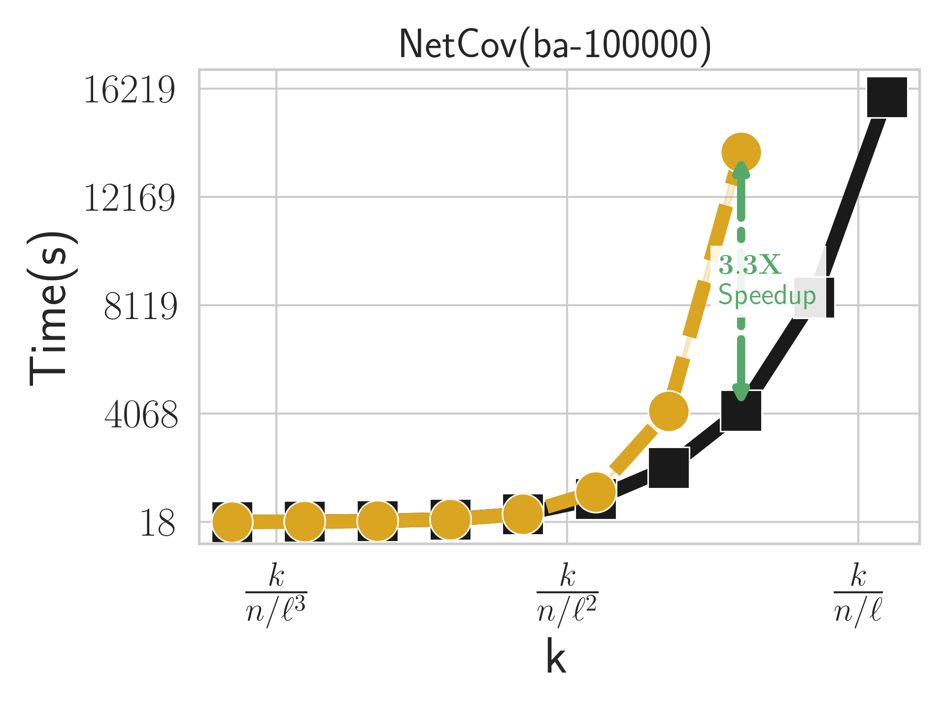
Figure 4 illustrates a linear speedup for R-DASH as the number of machines increases. Figure 4 highlights an intriguing observation that, despite having sufficient available memory, increasing can result in inferior performance when . Specifically, as depicted in Figure 4, we initially witness the expected faster execution of RandGreeDI with compared to RandGreeDI with . However, once , the relative performance of RandGreeDI with rapidly deteriorates. This decline can be attributed to the degradation of RandGreeDI’s optimal performance beyond .
When running RandGreeDI with a single thread on each machine, the total running time on machines can be computed based on two components. First, the running time for one machine in the first MR round, which is proportional to . Second, the running time for the primary machine in the second MR round (post-processing step), which is proportional to . Consequently, the total running time is proportional to . Optimal performance is achieved when , which justifies the preference for parallelization within a machine to maintain a lower rather than distributing the data across separate processors.
Furthermore, in Experiment 5 (Section 8.4), we demonstrate that utilizing MED enables MR algorithms to produce solutions much faster with no compromise in solution value, particularly when solving for . These results provide further support for the advantage of incorporating MED in achieving efficient and effective parallelization in MR algorithms.


8.4 Experiment 4 - Performance Analysis of MED


This section presents experimental results comparing the performance of MED+RG and the vanilla RandGreeDI algorithm. In terms of solution value, MED+RG consistently provides nearly identical solutions to the vanilla RandGreeDI algorithm across all instances for the three applications studied. Regarding runtime, the following observations are made: Initially, both algorithms exhibit similar execution times up to a threshold of . However, beyond this threshold, the performance gap between MED+RG and RandGreeDI widens linearly. MED+RG achieves notable average speedup factors of 1.8, 2.2, and 2.3 over RandGreeDI for the respective applications. Moreover, beyond , MED+RG outperforms RandGreeDI in terms of completing instances within a 12-hour timeout, completing 77% more instances of across all three applications. These findings highlight the promising performance of MED+RG, demonstrating comparable solution values while significantly improving runtime efficiency compared to the vanilla RandGreeDI algorithm.
The empirical findings from this experiment provide insights into the capabilities of the MED+Alg framework. Our results indicate that MED+Alg achieves solution quality that is practically indistinguishable from the vanilla Alg algorithm, even for significantly larger values of . Additionally, even with sufficient available memory to run Alg beyond , MED+Alg demonstrates noteworthy computational efficiency, surpassing that of the Alg algorithm. This combination of comparable solution quality and improved computational efficiency positions MED+Alg as a highly promising framework. These findings have significant implications and underscore the potential of MED+Alg to address complex problems in a distributed setting with large-scale values of .
9 Discussion and Conclusion
Prior to this work, no MR algorithms for SMCC could parallelize within a machine; these algorithms require many sequential queries. Moreover, increasing the number of machines to the number of threads available in the cluster may actually harm the performance, as we showed empirically; intuitively, this is because the size of the set on the primary machine scales linearly with the number of machines . In this paper, we have addressed this limitation by introducing a suite of algorithms that are both parallelizable and distributed. Specifically, we have presented R-DASH, T-DASH, and G-DASH, which are the first MR algorithms with sublinear adaptive complexity (highly parallelizable). Moreover, our algorithms make have nearly linear query complexity over the entire computation. We also provide the first distributed algorithm with total query complexity, improving on the of our other algorithms and the algorithm of Liu and Vondrak (2019).
When RandGreeDI was introduced by Mirzasoleiman et al. (2013), the empirical performance of the algorithm was emphasized, with theoretical guarantees unproven until the work of Barbosa et al. (2015). Since that time, RandGreeDI has remained the most practical algorithm for distributed SMCC. Our R-DASH algorithm may be regarded as a version of RandGreeDI that is 1) parallelized; 2) nearly linear time in total (RandGreeDI is quadratic); and 3) empirically orders of magnitude faster in parallel wall time in our evaluation.
R-DASH achieves approximation ratio of in two MR rounds; the first round merely being to distribute the data. We provide G-DASH to close the gap to ratio in a constant number of rounds. However, MR rounds are expensive (as shown by our Experiment 1). The current best ratio achieved in two rounds is the -approximation algorithm of Mirrokni and Zadimoghaddam (2015). Therefore, a natural question for future research is what is the best ratio achievable in two MR rounds. Moreover, non-monotone or partially monotone objective functions and more sophisticated constraint systems are directions for future research.
Acknowledgements
Yixin Chen and Tonmoy Dey contributed equally to this work. The work of Tonmoy Dey was partially supported by Florida State University; the work of Yixin Chen and Alan Kuhnle was partially supported by Texas A & M University. The authors have received no third-party funding in direct support of this work. The authors have no additional revenues from other sources related to this work.
Appendix A Lovász Extension of Submodular Function.
Given submodular function , the Lovász extension of is defined as follows: For ,
The Lovász extension satisfies the following properties: (1) is convex; (2) for any . Moreover, we will require the following simple lemma:
Lemma 8 (Barbosa et al. (2015)).
Let be a random set, and suppose , for . Then .
Appendix B Probability Lemma and Concentration Bounds
Lemma 9.
(Chen et al. (2021)) Suppose there is a sequence of Bernoulli trials: where the success probability of depends on the results of the preceding trials . Suppose it holds that
where is a constant and are arbitrary.
Then, if are independent Bernoulli trials, each with probability of success, then
where is an arbitrary integer.
Moreover, let be the first occurrence of success in sequence . Then,
Lemma 10 (Chernoff bounds Mitzenmacher and Upfal (2017)).
Suppose , … , are independent binary random variables such that . Let , and . Then for any , we have
| (8) |
Moreover, for any , we have
| (9) |
Appendix C Omitted Proof of ThreshSeqMod
See 2
Proof.
After filtration on Line 5, it holds that, for any , and . Therefore,
For any , it holds that . Due to submodularity, . Therefore, is subset of , which indicates that . ∎
Proof of Success Probability.
The algorithm successfully terminates if, at some point, or . To analyze the success probability, we consider a variant of the algorithm in which it does not terminate once or . In this case, the algorithm keeps running with and selecting empty set after inner for loop in the following iterations. Thus, with probability , either , or . Lemma 3 holds for all iterations of the outer for loop.
If the algorithm fails, there should be no more than successful iterations where . Otherwise, by Lemma 3, there exists an iteration such that , or . Let be the number of successful iterations. Then, is the sum of dependent Bernoulli random variables, where each variable has a success probability of more than . Let be the sum of independent Bernoulli random variables with success probability . By probability lemmata, the failure probability of Alg. 1 is calculated as follows,
| (Lemma 9) | ||||
| () | ||||
| (Lemma 10) | ||||
Proof of Adaptivity and Query Complexity.
Proof of Property (3).
For each iteration , consider two cases of by the choice of on Line 18. Firstly, if , clearly,
Secondly, if , let . Then, , and
Let , and . Then,
where the last inequality follows from . Therefore, by above two inequalities and monotonicity of ,
The objective value of the returned solution can be bounded as follows,
Proof of Property (4).
If the output set follows that , for any , it is filtered out at some point. Let be discarded at itetation . Then,
Appendix D ThresholdGreedy
In this section, we introduce a variant of near-linear time algorithm (Alg. 1) in Badanidiyuru and Vondrak (2014), ThresholdGreedy (Alg. 9), which requires two more parameters, constant and value . With the assumption that is an approximation solution, ThresholdGreedy ensures a approximation with query calls.
Theorem 8.
Let be an instance of SM, and is the optimal solution to . With input , and , where , ThresholdGreedy outputs solution with queries such that .
Proof.
Query Complexity. The while loop in Alg. 9 has at most iterations. For each iteration of the while loop, there are queries. Therefore, the query complexity of ThresholdGreedy is .
Approximation Ratio. If at termination, for any , it holds that . Then,
where Inequality (1) follows from monotonicity and submodularity.
If at termination, let be the intermediate solution after iteration of the while loop, and is the corresponding threshold. Suppose that . Then, each element added during iteration provides a minimum incremental benefit of ,
Next, we consider iteration . If , since the algorithm does not terminate during iteration , each element in is either added to the solution or omitted due to small marginal gain with respect to the current solution. Therefore, for any , it holds that by submodularity. Then,
If , and .
Therefore, for any iteration that has elements being added to the solution, it holds that
| () | ||||
| () |
. Application Small Data Large Data Edges Edges ImageSumm 10,000 50,000 InfluenceMax 26,588 1,134,890 RevenueMax 17,432 3,072,441 MaxCover (BA) 100,000 1,000,000
Appendix E Threshold-DASH with no Knowledge of OPT
See 7
Proof.
By Definition ( in Section 5), it holds that . Since is assigned to each machine randomly with probability ,
Moreover, we know that any two machines selects elements independently. So,
where Inequality (a) follows from .
Thus, we can bound the probability by the following,
∎
Description. The T-DASH algorithm described in Alg. 10 is a two MR-rounds algorithm using the AFD approach that runs ThreshSeqMod concurrently on every machine for different guesses of threshold in the range ; where is the approximation of T-DASH and is the maximum singleton in . Every solution returned to the primary machine are placed into bins based on their corresponding threshold guess such that ; where is the maximum singleton in . Since there must exist a threshold that is close enough to ; running ThreshSeqMod (Line 21) on every bin in the range and selecting the best solution guarantees the -approximation of T-DASH in adaptive rounds.
Theorem 9.
Let be an instance of SM where . T-DASH with no knowledge of OPT returns set with two MR rounds, adaptive rounds, total queries, communication complexity, and probability at least such that
Overview of Proof. Alg. 10 is inspired by Alg. 6 in Section 5, which is a version of the algorithm that knows that optimal solution value. With , there exists an such that with guesses. Then, on each machine , we only consider sets and such that . If this does exist, works like in Alg. 6. If this does not exist, then for any , it holds that , which means with will return an empty set. Since each call of ThreshSeqMod with different guesses on is executed in parallel, the adaptivity remains the same and the query complexity increases by a factor of .
Proof.
First, for , ; and for ,
Therefore, there exists an such that . Since , it holds that and .
Then, we only consider . If , by Theorem 1, it holds that,
Otherwise, in the case that , let , . Also, let be returned by machine that , define
On the machine which does not return a , we consider it runs and returns two empty sets, and hence . Let , . Then, Lemma 7 in Appendix E still holds in this case. We can calculate the approximation ratio as follows with ,
∎
Appendix F Experiment Setup
F.1 Applications
Given a constraint , the objectives of the applications are defined as follows:
F.1.1 Max Cover
Maximize the number of nodes covered by choosing a set of maximum size , such that the number of nodes having at least one neighbour in the set . The application is run on synthetic random BA graphs of groundset size 100,000, 1,000,000 and 5,000,000 generated using Barabási–Albert (BA) models for the centralized and distributed experiments respectively.
F.1.2 Image Summarization on CIFAR-10 Data
Given large collection of images, find a subset of maximum size which is representative of the entire collection. The objective used for the experiments is a monotone variant of the image summarization from Fahrbach et al. (2019b). For a groundset with images, it is defined as follows:
where is the cosine similarity of the pixel values between image and image . The data for the image summarization experiments contains 10,000 and 50,000 CIFAR-10 Krizhevsky et al. (2009) color images respectively for the centralized and distributed experiments.
F.1.3 Influence Maximization on a Social Network.
Maximise the aggregate influence to promote a topic by selecting a set of social network influencers of maximum size . The probability that a random user will be influenced by the set of influencers in is given by:
where —— is the number of neighbors of node in . We use the Epinions data set consisting of 27,000 users from Rossi and Ahmed (2015) for the centralized data experiments and the Youtube online social network data Yang and Leskovec (2012) consisting more than 1 million users for distrbuted data experiments. The value of is set to 0.01.
F.1.4 Revenue Maximization on YouTube.
Maximise revenue of a product by selecting set of users of maximum size , where the network neighbors will be advertised a different product by the set of users . It is based on the objective function from Mirzasoleiman et al. (2016). For a given set of users and as the influence between user and , the objective function can be defined by:
where , the expected revenue from an user is a function of the sum of influences from neighbors who are in and is a rate of diminishing returns parameter for increased cover.
We use the Youtube data set from Mirzasoleiman et al. (2016) consisting of 18,000 users for centralized data experiments. For the distrbuted data experiments we perform empirical evaluation on the Orkut online social network data from Yang and Leskovec (2012) consisting more than 3 million users. The value of is set to 0.3
Appendix G Replicating the Experiment Results
Our experiments can be replicated by running the following scripts:
-
•
Install MPICH version 3.3a2 (DO NOT install OpenMPI and ensure mpirun utlizes mpich using the command mpirun –version (Ubuntu))
-
•
Install pandas, mpi4py, scipy, networkx
-
•
Set up an MPI cluster using the following tutorial:
https://mpitutorial.com/tutorials/running-an-mpi-cluster-within-a-lan/ -
•
Create and update the host file ../nodesFileIPnew to store the ip addresses of all the connected MPI machines before running any experiments (First machine being the primary machine)
-
–
NOTE: Please place nodesFileIPnew inside the MPI shared repository; ”cloud/” in this case (at the same level as the code base directory). DO NOT place it inside the code base ”DASH-Distributed_SMCC-python/” directory.
-
–
-
•
Clone the DASH-Distributed_SMCC-python repository inside the MPI shared repository (/cloud in the case using the given tutorial)
-
–
NOTE: Please clone the ”DASH-Distributed_SMCC-python” repository and execute the following commands on a machine with sufficient memory (RAM); capable of generating the large datasets. This repository NEED NOT be the primary repository (”/cloud/DASH-Distributed_SMCC-python/”) on the shared memory of the cluster; that will be used for the experiments.
-
–
-
•
Additional Datasets For Experiment 1 : Please download the Image Similarity Matrix file ”images_10K_mat.csv”(https://drive.google.com/file/d/1s9PzUhV-C5dW8iL4tZPVjSRX4PBhrsiJ/view?usp=sharing)) and place it in the data/data_exp1/ directory.
-
•
To generate the decentralized data for Experiment 2 and 3 : Please follow the below steps:
-
–
Execute bash GenerateDistributedData.bash nThreads nNodes
-
–
The previous command should generate nNodes directories in loading_data/ directory (with names machinenodeNoData)
-
–
Copy the data_exp2_split/ and data_exp3_split/ directories within each machineiData directory to the corresponding machine and place the directories outside /cloud (directory created after setting up an MPI cluster using the given tutorial)).
-
–
To run all experiments in the apper
Please read the README.md file in the ”DASH-Distributed_SMCC-python” (Code/Data Appendix) for detailed information.
Appendix H The Greedy Algorithm (Nemhauser and Wolsey (1978))
The standard Greedy algorithm starts with an empty set and then proceeds by adding elements to the set over iterations. In each iteration the algorithm selects the element with the maximum marginal gain where . The Algorithm 11 is a formal statement of the standard Greedy algorithm. The intermediate solution set represents the solution after iteration . The ( 0.632)-approximation of the Greedy algorithm is the optimal ratio possible for monotone objectives.
Appendix I Discussion of the -approximate Algorithm in Liu and Vondrak (2019)
The simple two-round distributed algorithm proposed by Liu and Vondrak (2019) achieves a deterministic approximation ratio. The pseudocode of this algorithm, assuming that we know OPT, is provided in Alg. 14. The guessing OPT version runs copies of Alg. 14 on each machine, which has adaptivity and query complexity.
Intuitively, the result of Alg. 14 is equivalent to a single run of ThresholdGreedy on the whole ground set. Within the first round, it calls ThresholdGreedy on to get an intermediate solution . After filtering out the elements with gains less than in , the rest of the elements in are sent to the primary machine. By careful analysis, there is a high probability that the total number of elements returned within the first round is less than .
Compared to the 2-round algorithms in Table 1, Alg. 14 is the only algorithm that requires data duplication, with four times more elements distributed to each machine in the first round. As a result, distributed setups have a more rigid memory restriction when running this algorithm. For example, when the dataset exactly fits into the distributed setups which follows that , there is no more space on each machine to store the random subset . In the meantime, other 2-round algorithms can still run with .
Additionally, since the approximation analysis of Alg. 14 does not take randomization into consideration, we may be able to substitute its ThresholdGreedy subroutine with any threshold algorithm (such as ThresholdSeq in Chen et al. (2021)) that has optimal logarithmic adaptivity and linear query complexity. However, given its analysis of the success probability considers as blocks where each block has random access to the whole ground set, it may not be easy to fit parallelizable threshold algorithms into this framework.
References
- Badanidiyuru and Vondrak (2014) Ashwinkumar Badanidiyuru and Jan Vondrak. Fast algorithms for maximizing submodular functions. In Chandra Chekuri, editor, Proceedings of the Twenty-Fifth Annual ACM-SIAM Symposium on Discrete Algorithms, SODA 2014, Portland, Oregon, USA, January 5-7, 2014, pages 1497–1514. SIAM, 2014.
- Balakrishnan et al. (2022) Ravikumar Balakrishnan, Tian Li, Tianyi Zhou, Nageen Himayat, Virginia Smith, and Jeff A. Bilmes. Diverse client selection for federated learning via submodular maximization. In The Tenth International Conference on Learning Representations, ICLR 2022, Virtual Event, April 25-29, 2022, 2022.
- Balkanski and Singer (2018) Eric Balkanski and Yaron Singer. The adaptive complexity of maximizing a submodular function. In Ilias Diakonikolas, David Kempe, and Monika Henzinger, editors, Proceedings of the 50th Annual ACM SIGACT Symposium on Theory of Computing, STOC 2018, Los Angeles, CA, USA, June 25-29, 2018, pages 1138–1151. ACM, 2018.
- Balkanski et al. (2019) Eric Balkanski, Aviad Rubinstein, and Yaron Singer. An exponential speedup in parallel running time for submodular maximization without loss in approximation. In Timothy M. Chan, editor, Proceedings of the Thirtieth Annual ACM-SIAM Symposium on Discrete Algorithms, SODA 2019, San Diego, California, USA, January 6-9, 2019, pages 283–302. SIAM, 2019.
- Barbosa et al. (2015) Rafael da Ponte Barbosa, Alina Ene, Huy L. Nguyen, and Justin Ward. The power of randomization: Distributed submodular maximization on massive datasets. In Francis R. Bach and David M. Blei, editors, Proceedings of the 32nd International Conference on Machine Learning, ICML 2015, Lille, France, 6-11 July 2015, volume 37 of JMLR Workshop and Conference Proceedings, pages 1236–1244. JMLR.org, 2015.
- Barbosa et al. (2016) Rafael da Ponte Barbosa, Alina Ene, Huy L. Nguyen, and Justin Ward. A new framework for distributed submodular maximization. In Irit Dinur, editor, IEEE 57th Annual Symposium on Foundations of Computer Science, FOCS 2016, 9-11 October 2016, Hyatt Regency, New Brunswick, New Jersey, USA, pages 645–654. IEEE Computer Society, 2016.
- Blelloch et al. (2012) Guy E. Blelloch, Harsha Vardhan Simhadri, and Kanat Tangwongsan. Parallel and I/O efficient set covering algorithms. In Guy E. Blelloch and Maurice Herlihy, editors, 24th ACM Symposium on Parallelism in Algorithms and Architectures, SPAA ’12, Pittsburgh, PA, USA, June 25-27, 2012, pages 82–90. ACM, 2012.
- Breuer et al. (2020) Adam Breuer, Eric Balkanski, and Yaron Singer. The FAST algorithm for submodular maximization. In Proceedings of the 37th International Conference on Machine Learning, ICML 2020, 13-18 July 2020, Virtual Event, volume 119 of Proceedings of Machine Learning Research, pages 1134–1143. PMLR, 2020.
- Buchbinder et al. (2014) Niv Buchbinder, Moran Feldman, Joseph Naor, and Roy Schwartz. Submodular maximization with cardinality constraints. In Chandra Chekuri, editor, Proceedings of the Twenty-Fifth Annual ACM-SIAM Symposium on Discrete Algorithms, SODA 2014, Portland, Oregon, USA, January 5-7, 2014, pages 1433–1452. SIAM, 2014.
- Buchbinder et al. (2017) Niv Buchbinder, Moran Feldman, and Roy Schwartz. Comparing apples and oranges: Query trade-off in submodular maximization. Math. Oper. Res., 42(2):308–329, 2017.
- Calinescu et al. (2007) Gruia Calinescu, Chandra Chekuri, Martin Pal, and Jan Vondrak. Maximizing a submodular set function subject to a matroid constraint (extended abstract). In Matteo Fischetti and David P. Williamson, editors, Integer Programming and Combinatorial Optimization, 12th International IPCO Conference, Ithaca, NY, USA, June 25-27, 2007, Proceedings, volume 4513 of Lecture Notes in Computer Science, pages 182–196. Springer, 2007.
- Chekuri and Quanrud (2019) Chandra Chekuri and Kent Quanrud. Submodular function maximization in parallel via the multilinear relaxation. In Timothy M. Chan, editor, Proceedings of the Thirtieth Annual ACM-SIAM Symposium on Discrete Algorithms, SODA 2019, San Diego, California, USA, January 6-9, 2019, pages 303–322. SIAM, 2019.
- Chen and Kuhnle (2024) Yixin Chen and Alan Kuhnle. Practical and parallelizable algorithms for non-monotone submodular maximization with size constraint. J. Artif. Intell. Res., 79:599–637, 2024.
- Chen et al. (2021) Yixin Chen, Tonmoy Dey, and Alan Kuhnle. Best of both worlds: Practical and theoretically optimal submodular maximization in parallel. In Marc’Aurelio Ranzato, Alina Beygelzimer, Yann N. Dauphin, Percy Liang, and Jennifer Wortman Vaughan, editors, Advances in Neural Information Processing Systems 34: Annual Conference on Neural Information Processing Systems 2021, NeurIPS 2021, December 6-14, 2021, virtual, pages 25528–25539, 2021.
- Chierichetti et al. (2010) Flavio Chierichetti, Ravi Kumar, and Andrew Tomkins. Max-cover in map-reduce. In Michael Rappa, Paul Jones, Juliana Freire, and Soumen Chakrabarti, editors, Proceedings of the 19th International Conference on World Wide Web, WWW 2010, Raleigh, North Carolina, USA, April 26-30, 2010, pages 231–240. ACM, 2010.
- Dey et al. (2023) Tonmoy Dey, Yixin Chen, and Alan Kuhnle. DASH: A distributed and parallelizable algorithm for size-constrained submodular maximization. In Brian Williams, Yiling Chen, and Jennifer Neville, editors, Thirty-Seventh AAAI Conference on Artificial Intelligence, AAAI 2023, Thirty-Fifth Conference on Innovative Applications of Artificial Intelligence, IAAI 2023, Thirteenth Symposium on Educational Advances in Artificial Intelligence, EAAI 2023, Washington, DC, USA, February 7-14, 2023, pages 3941–3948. AAAI Press, 2023.
- Ene and Nguyen (2019) Alina Ene and Huy L. Nguyen. Submodular maximization with nearly-optimal approximation and adaptivity in nearly-linear time. In Timothy M. Chan, editor, Proceedings of the Thirtieth Annual ACM-SIAM Symposium on Discrete Algorithms, SODA 2019, San Diego, California, USA, January 6-9, 2019, pages 274–282. SIAM, 2019.
- Ene and Nguyen (2020) Alina Ene and Huy L. Nguyen. Parallel algorithm for non-monotone dr-submodular maximization. In Proceedings of the 37th International Conference on Machine Learning, ICML 2020, 13-18 July 2020, Virtual Event, volume 119 of Proceedings of Machine Learning Research, pages 2902–2911. PMLR, 2020.
- Epasto et al. (2017) Alessandro Epasto, Vahab S. Mirrokni, and Morteza Zadimoghaddam. Bicriteria distributed submodular maximization in a few rounds. In Christian Scheideler and Mohammad Taghi Hajiaghayi, editors, Proceedings of the 29th ACM Symposium on Parallelism in Algorithms and Architectures, SPAA 2017, Washington DC, USA, July 24-26, 2017, pages 25–33. ACM, 2017.
- Ettinger et al. (2021) Scott Ettinger, Shuyang Cheng, Benjamin Caine, Chenxi Liu, Hang Zhao, Sabeek Pradhan, Yuning Chai, Ben Sapp, Charles R. Qi, Yin Zhou, Zoey Yang, Aurelien Chouard, Pei Sun, Jiquan Ngiam, Vijay Vasudevan, Alexander McCauley, Jonathon Shlens, and Dragomir Anguelov. Large scale interactive motion forecasting for autonomous driving : The waymo open motion dataset. In 2021 IEEE/CVF International Conference on Computer Vision, ICCV 2021, Montreal, QC, Canada, October 10-17, 2021, pages 9690–9699. IEEE, 2021.
- Fahrbach et al. (2019a) Matthew Fahrbach, Vahab S. Mirrokni, and Morteza Zadimoghaddam. Submodular maximization with nearly optimal approximation, adaptivity and query complexity. In Timothy M. Chan, editor, Proceedings of the Thirtieth Annual ACM-SIAM Symposium on Discrete Algorithms, SODA 2019, San Diego, California, USA, January 6-9, 2019, pages 255–273. SIAM, 2019a.
- Fahrbach et al. (2019b) Matthew Fahrbach, Vahab S. Mirrokni, and Morteza Zadimoghaddam. Non-monotone submodular maximization with nearly optimal adaptivity and query complexity. In Kamalika Chaudhuri and Ruslan Salakhutdinov, editors, Proceedings of the 36th International Conference on Machine Learning, ICML 2019, 9-15 June 2019, Long Beach, California, USA, volume 97 of Proceedings of Machine Learning Research, pages 1833–1842. PMLR, 2019b.
- Gupta et al. (2010) Anupam Gupta, Aaron Roth, Grant Schoenebeck, and Kunal Talwar. Constrained non-monotone submodular maximization: Offline and secretary algorithms. In Amin Saberi, editor, Internet and Network Economics - 6th International Workshop, WINE 2010, Stanford, CA, USA, December 13-17, 2010. Proceedings, volume 6484 of Lecture Notes in Computer Science, pages 246–257. Springer, 2010.
- Joseph et al. (2019) K. J. Joseph, Vamshi Teja R, Krishnakant Singh, and Vineeth N. Balasubramanian. Submodular batch selection for training deep neural networks. In Sarit Kraus, editor, Proceedings of the Twenty-Eighth International Joint Conference on Artificial Intelligence, IJCAI 2019, Macao, China, August 10-16, 2019, pages 2677–2683. ijcai.org, 2019.
- Kazemi et al. (2019) Ehsan Kazemi, Marko Mitrovic, Morteza Zadimoghaddam, Silvio Lattanzi, and Amin Karbasi. Submodular streaming in all its glory: Tight approximation, minimum memory and low adaptive complexity. In Kamalika Chaudhuri and Ruslan Salakhutdinov, editors, Proceedings of the 36th International Conference on Machine Learning, ICML 2019, 9-15 June 2019, Long Beach, California, USA, volume 97 of Proceedings of Machine Learning Research, pages 3311–3320. PMLR, 2019.
- Kazemi et al. (2021) Ehsan Kazemi, Shervin Minaee, Moran Feldman, and Amin Karbasi. Regularized submodular maximization at scale. In Marina Meila and Tong Zhang, editors, Proceedings of the 38th International Conference on Machine Learning, ICML 2021, 18-24 July 2021, Virtual Event, volume 139 of Proceedings of Machine Learning Research, pages 5356–5366. PMLR, 2021.
- Krizhevsky et al. (2009) Alex Krizhevsky, Geoffrey Hinton, et al. Learning multiple layers of features from tiny images. In University of Toronto, Canada. Citeseer, 2009.
- Kuhnle (2021) Alan Kuhnle. Quick streaming algorithms for maximization of monotone submodular functions in linear time. In Arindam Banerjee and Kenji Fukumizu, editors, The 24th International Conference on Artificial Intelligence and Statistics, AISTATS 2021, April 13-15, 2021, Virtual Event, volume 130 of Proceedings of Machine Learning Research, pages 1360–1368. PMLR, 2021.
- Kumar et al. (2013) Ravi Kumar, Benjamin Moseley, Sergei Vassilvitskii, and Andrea Vattani. Fast greedy algorithms in mapreduce and streaming. In Guy E. Blelloch and Berthold Vöcking, editors, 25th ACM Symposium on Parallelism in Algorithms and Architectures, SPAA ’13, Montreal, QC, Canada - July 23 - 25, 2013, pages 1–10. ACM, 2013.
- Lee et al. (2009) Jon Lee, Vahab S. Mirrokni, Viswanath Nagarajan, and Maxim Sviridenko. Non-monotone submodular maximization under matroid and knapsack constraints. In Michael Mitzenmacher, editor, Proceedings of the 41st Annual ACM Symposium on Theory of Computing, STOC 2009, Bethesda, MD, USA, May 31 - June 2, 2009, pages 323–332. ACM, 2009.
- Liu and Vondrak (2019) Paul Liu and Jan Vondrak. Submodular optimization in the mapreduce model. In Jeremy T. Fineman and Michael Mitzenmacher, editors, 2nd Symposium on Simplicity in Algorithms, SOSA 2019, January 8-9, 2019, San Diego, CA, USA, volume 69 of OASIcs, pages 18:1–18:10. Schloss Dagstuhl - Leibniz-Zentrum für Informatik, 2019.
- Liu (2020) Siwen Liu. A review for submodular optimization on machine scheduling problems. In Ding-Zhu Du and Jie Wang, editors, Complexity and Approximation - In Memory of Ker-I Ko, volume 12000 of Lecture Notes in Computer Science, pages 252–267. Springer, 2020.
- Liu et al. (2020) Yajing Liu, Edwin K. P. Chong, Ali Pezeshki, and Zhenliang Zhang. Submodular optimization problems and greedy strategies: A survey. Discret. Event Dyn. Syst., 30(3):381–412, 2020.
- Mao et al. (2021) Jiageng Mao, Minzhe Niu, Chenhan Jiang, Hanxue Liang, Jingheng Chen, Xiaodan Liang, Yamin Li, Chaoqiang Ye, Wei Zhang, Zhenguo Li, Jie Yu, Chunjing Xu, and Hang Xu. One million scenes for autonomous driving: ONCE dataset. In Joaquin Vanschoren and Sai-Kit Yeung, editors, Proceedings of the Neural Information Processing Systems Track on Datasets and Benchmarks 1, NeurIPS Datasets and Benchmarks 2021, December 2021, virtual, 2021.
- Mirrokni and Zadimoghaddam (2015) Vahab S. Mirrokni and Morteza Zadimoghaddam. Randomized composable core-sets for distributed submodular maximization. In Rocco A. Servedio and Ronitt Rubinfeld, editors, Proceedings of the Forty-Seventh Annual ACM on Symposium on Theory of Computing, STOC 2015, Portland, OR, USA, June 14-17, 2015, pages 153–162. ACM, 2015.
- Mirzasoleiman et al. (2013) Baharan Mirzasoleiman, Amin Karbasi, Rik Sarkar, and Andreas Krause. Distributed submodular maximization: Identifying representative elements in massive data. In Christopher J. C. Burges, Léon Bottou, Zoubin Ghahramani, and Kilian Q. Weinberger, editors, Advances in Neural Information Processing Systems 26: 27th Annual Conference on Neural Information Processing Systems 2013. Proceedings of a meeting held December 5-8, 2013, Lake Tahoe, Nevada, United States, pages 2049–2057, 2013.
- Mirzasoleiman et al. (2015) Baharan Mirzasoleiman, Ashwinkumar Badanidiyuru, Amin Karbasi, Jan Vondrak, and Andreas Krause. Lazier than lazy greedy. In Blai Bonet and Sven Koenig, editors, Proceedings of the Twenty-Ninth AAAI Conference on Artificial Intelligence, January 25-30, 2015, Austin, Texas, USA, pages 1812–1818. AAAI Press, 2015.
- Mirzasoleiman et al. (2016) Baharan Mirzasoleiman, Ashwinkumar Badanidiyuru, and Amin Karbasi. Fast constrained submodular maximization: Personalized data summarization. In Maria-Florina Balcan and Kilian Q. Weinberger, editors, Proceedings of the 33nd International Conference on Machine Learning, ICML 2016, New York City, NY, USA, June 19-24, 2016, volume 48 of JMLR Workshop and Conference Proceedings, pages 1358–1367. JMLR.org, 2016.
- Mirzasoleiman et al. (2018) Baharan Mirzasoleiman, Stefanie Jegelka, and Andreas Krause. Streaming non-monotone submodular maximization: Personalized video summarization on the fly. In Sheila A. McIlraith and Kilian Q. Weinberger, editors, Proceedings of the Thirty-Second AAAI Conference on Artificial Intelligence, (AAAI-18), the 30th innovative Applications of Artificial Intelligence (IAAI-18), and the 8th AAAI Symposium on Educational Advances in Artificial Intelligence (EAAI-18), New Orleans, Louisiana, USA, February 2-7, 2018, pages 1379–1386. AAAI Press, 2018.
- Mitzenmacher and Upfal (2017) Michael Mitzenmacher and Eli Upfal. Probability and computing: Randomization and probabilistic techniques in algorithms and data analysis. Cambridge university press, 2017.
- Nemhauser and Wolsey (1978) George L. Nemhauser and Laurence A. Wolsey. Best algorithms for approximating the maximum of a submodular set function. Math. Oper. Res., 3(3):177–188, 1978.
- Nemhauser et al. (1978) George L. Nemhauser, Laurence A. Wolsey, and Marshall L. Fisher. An analysis of approximations for maximizing submodular set functions - I. Math. Program., 14(1):265–294, 1978.
- Rangwani et al. (2021) Harsh Rangwani, Arihant Jain, Sumukh K. Aithal, and R. Venkatesh Babu. Svaada: Submodular subset selection for virtual adversarial active domain adaptation. In 2021 IEEE/CVF International Conference on Computer Vision, ICCV 2021, Montreal, QC, Canada, October 10-17, 2021, pages 7496–7505. IEEE, 2021.
- Rossi and Ahmed (2015) Ryan A. Rossi and Nesreen K. Ahmed. The network data repository with interactive graph analytics and visualization. In Blai Bonet and Sven Koenig, editors, Proceedings of the Twenty-Ninth AAAI Conference on Artificial Intelligence, January 25-30, 2015, Austin, Texas, USA, pages 4292–4293. AAAI Press, 2015.
- Yang and Leskovec (2012) Jaewon Yang and Jure Leskovec. Defining and evaluating network communities based on ground-truth. In Mohammed Javeed Zaki, Arno Siebes, Jeffrey Xu Yu, Bart Goethals, Geoffrey I. Webb, and Xindong Wu, editors, 12th IEEE International Conference on Data Mining, ICDM 2012, Brussels, Belgium, December 10-13, 2012, pages 745–754. IEEE Computer Society, 2012.