This paper was converted on www.awesomepapers.org from LaTeX by an anonymous user.
Want to know more? Visit the Converter page.

Scalable and Sample Efficient Distributed Policy Gradient Algorithms in Multi-Agent Networked Systems

Xin Liu
ShanghaiTech University
[email protected]
   Honghao Wei
University of Michigan, Ann Arbor
[email protected]
   Lei Ying
University of Michigan, Ann Arbor
[email protected]
Abstract

This paper studies a class of multi-agent reinforcement learning (MARL) problems where the reward that an agent receives depends on the states of other agents, but the next state only depends on the agent’s own current state and action. We name it REC-MARL standing for REward-Coupled Multi-Agent Reinforcement Learning. REC-MARL has a range of important applications such as real-time access control and distributed power control in wireless networks. This paper presents a distributed policy gradient algorithm for REC-MARL. The proposed algorithm is distributed in two aspects: (i) the learned policy is a distributed policy that maps a local state of an agent to its local action and (ii) the learning/training is distributed, during which each agent updates its policy based on its own and neighbors’ information. The learned algorithm achieves a stationary policy and its iterative complexity bounds depend on the dimension of local states and actions. The experimental results of our algorithm for the real-time access control and power control in wireless networks show that our policy significantly outperforms the state-of-the-art algorithms and well-known benchmarks.

1 Introduction

Multi-Agent Reinforcement Learning, or MARL for short, considers a reinforcement learning problem where multiple agents interact with each other and with the environment to finish a common task or achieve a common objective. The key difference between MARL and single-agent RL is that each agent in MARL only observes a subset of the state and receives an individual reward and does not have global information. Examples include multi-access networks where each user senses the collision locally, but needs to coordinate with each other to maximize the network throughput, or power control in wireless networks where each wireless node can only measure its local interference but they need to collectively decide the transmit power levels to maximize a network-wide utility, or task offloading in edge computing where each user observes its local quality of service (QoS) but they coordinate tasks offloaded to edge servers to maintain a high QoS for the network, or a team of robots where each robot can only sense its own surrounding environment, but the robot team needs to cooperate and coordinate for accomplishing a rescue task.

MARL raises two fundamental aspects that are different from single-agent RL. The first aspect is the policy space (the set of policies that are feasible) is restricted to local policies since each agent has to decide an action based on information available to the agent. The second aspect of MARL is that while distributed learning, e.g. distributed policy gradient, is desired, it is impossible in general MARL because an agent does not know the global state and rewards. One popular approach to address the second issue is the centralized learning and distributed execution paradigm [8], where data samples are collected by a central entity and the central entity uses data from all agents to learn a local policy. Therefore, the learning occurs at the central entity, but the learned policy is a local policy.

In this paper, we consider a special class of MARL, which we call REward-Coupled Multi-Agent Reinforcement Learning (REC-MARL). In REC-MARL, the problem is coupled through the reward functions. More specifically, the reward function of agent nn depends on agent nn’s state and action and its neighbors’ states and actions. However, the next state of agent nn only depends on agent nn^{\prime}s current state and action, and is independent of other agents’ states and actions. In contrast, in general MARL, the transition kernels of the agents are coupled, so the next state of an agent depends on other agents’ states and actions.

While REC-MARL is more restrictive than MARL, a number of applications of MARL are actually REC-MARL. In wireless networks, where agents are network nodes or devices, and the state of an agent is could be its queue length or transmit power, the state only depends on an agent’s current state and its current action (see Section 2 for detailed description). For REC-MARL, this paper proposes distributed policy gradient algorithms and establish the local convergence (i.e. the algorithms achieve a stationary policy). The main contributions are summarized as follows.

  • We establish perfect decomposition of value functions and policy gradients in Lemmas 1 and 2, respectively, where we show that the global value functions (policy-gradients) can be written as a summation of local value functions (policy gradients). This decomposition significantly reduces the complexity of value functions and motivates our distributed multi-agent policy gradient algorithms.

  • We propose a Temporal-Difference (TD) learning based regularized distributed multi-agent policy gradient algorithm, named TD-RDAC in Algorithm 2. We proved in Theorem 2 that TD-RDAC achieves the local convergence with the rate O~(NSmaxAmax/T),\tilde{O}\left(NS_{\max}A_{\max}/\sqrt{T}\right), which only depends on the maximum sizes of local state and action spaces, instead of the sizes of the global action and state spaces.

  • We apply TD-RDAC to the applications of real-time access and power control in ad hoc wireless networks, both are well-known challenging networking resource management problems. Our experiments show that TD-RDAC significantly outperforms the state-of-the-art algorithm [20] and well-known benchmarks [2, 21] in these two applications.

Related Work

MARL for networking: MARL have been applied to various networking applications (e.g., content caching [25], packet routing [23], video transcoding and transmission [3], transportation network control [6]). The work [25] proposed a multi-agent advantage actor-critic algorithm for large-scale video caching at network edge and it reduced the content access latency and traffic cost. The proposed algorithm requires the knowledge of neighbors’ policies, which is usually not observable. [23] studied packet routing problem in WAN and applied MARL to minimize the average packet completion time. The method adopted dynamic consensus algorithm to estimate the global reward, which incurs a heavy communication overhead. The work [3] proposed a multi-agent actor-critic algorithm for crowd-sourced livecast services and improved the average throughput and the transmission delay performance. The proposed algorithm requires a centralized controller to maintain the global state information. The most related work is [6], which utilized spatial discount factor to decouple the correlation of distant agents and designed networked MARL solution in traffic signal control and cooperative cruise control. However, it requires a dedicated communication module to maintain a local estimation of global state, which again incurs large communication cost. Moreover, the theoretical performance of these algorithms in [25, 23, 3, 6] are not investigated.

Provable MARL: There have been a great amount of works addressing the issues of scalability and sample complexity in MARL. A popular paradigm is the centralized learning and distributed execution (see e.g. [8]), where agents share a centralized critic but have individual actors. Both the critic and the actors are trained at a central server, but the actors are local policies that lead to a distributed implementation. [29] proposed a decentralized actor-critic algorithm for a cooperative scenario, where each agent has its individual critic and actor with a shared global state. The proposed algorithm converges an stationary point of the objective function. Motivated by [29], [4] and [10] provided a finite-time analysis of decentralized actor-critic algorithms in the infinity-horizon discounted-reward MDPs and average-reward MDPs, respectively. [30] studied a policy gradient algorithm for multi-agent stochastic games, where each agent maximizes its reward by taking actions independently based on the global state. It established its local convergence for general stochastic games and its global convergence for Markov potential games. The centralized critic or shared states (even with decentralized actors) require collecting global information and centralized training. The work [19] exploits the network structure to develop a localized or scalable actor-critic (SAC) framework that is proved to achieve O(γk+1)O(\gamma^{k+1})-approximation of a stationary point in γ\gamma-discounted-reward MDPs. [20] and [13] extended SAC framework in [19] into the settings of infinity-horizon average-reward MDPs and stochastic/time-varying communication graphs. The SAC framework in [19] is efficient in implementing the paradigm of distributed learning and distributed execution. It is also worth mentioning that in a recent work [31], the authors studied a kernel-coupled setting and established that the localized policy-gradient converges to a neighborhood of global optimal policy, where the distance to the global optimality depends on the number of hops, kk, polynomially and could be a constant when kk is small. Another line of research in MARL that addresses the scalability issue is the mean-field approximation (MFA) [9, 7, 27], where agents are homogeneous and an individual agent interacts or games with the approximated “mean” behavior. However, the MFA approach is only applicable to a homogeneous system. Finally, [16] and [26] studied weakly-coupled MDPs, where individual MDPs are independent and coupled through constraints, instead of coupled reward as in ours.

Different from these existing works, this paper considers reward-coupled multi-agent Reinforcement learning (REC-MARL), establishes the local convergence of policy gradient algorithms with both distributed learning and distributed implementation, and demonstrates its efficiency in classical and challenging resource management problems.

2 Model

We consider a multi-agent system where the agents are connected by an interactive graph 𝒢=(,)\mathcal{G}=(\mathcal{I},\mathcal{E}) with \mathcal{I} and \mathcal{E} being the set of nodes and edges, respectively. The system consists of N=||N=|\mathcal{I}| agents who are connected with edges in .\mathcal{E}. Each agent nn\in\mathcal{I} is associated with a γ\gamma-discounted Markov decision process of (𝒮n,𝒜n,rn,𝒫n,γ),(\mathcal{S}_{n},\mathcal{A}_{n},r_{n},\mathcal{P}_{n},\gamma), where 𝒮n\mathcal{S}_{n} is the state space, 𝒜n\mathcal{A}_{n} is the action space, rnr_{n} is the reward function, and 𝒫n\mathcal{P}_{n} is the transition kernel. Define the neighbourhood of agent nn (including itself) to be 𝒩(n).\mathcal{N}(n). Define the states and actions of the neighbors of agent nn to be s𝒩(n)s_{\mathcal{N}(n)} and a𝒩(n),a_{\mathcal{N}(n)}, respectively. We next formally define the REward-Couple Multi-Agent Reinforcement Learning.

REC-MARL: The reward of agent nn depends on its neighbors’ states and actions rn(s𝒩(n),a𝒩(n)).r_{n}(s_{\mathcal{N}(n)},a_{\mathcal{N}(n)}). The transition kernel of agent n,n, 𝒫n(|sn,an),\mathcal{P}_{n}(\cdot|s_{n},a_{n}), only depends on its own state sns_{n} and action an.a_{n}. Agent nn uses a local policy πn:𝒮n𝒜n,\pi_{n}:\mathcal{S}_{n}\to\mathcal{A}_{n}, where πn(an|sn)\pi_{n}(a_{n}|s_{n}) is the probability of taking action ana_{n} in state sn.s_{n}.

Given a REC-MARL problem, the global state space is 𝒮=𝒮1×𝒮2××𝒮n\mathcal{S}=\mathcal{S}_{1}\times\mathcal{S}_{2}\times\cdots\times\mathcal{S}_{n} with Smax=maxn|𝒮n|;S_{\max}=\max_{n}|\mathcal{S}_{n}|; the global action space is 𝒜=𝒜1×𝒜2××𝒜n\mathcal{A}=\mathcal{A}_{1}\times\mathcal{A}_{2}\times\cdots\times\mathcal{A}_{n} with Amax=maxn|𝒜n|;A_{\max}=\max_{n}|\mathcal{A}_{n}|; the global reward function is r(s,a)=1Nn=1Nrn(s𝒩(n),a𝒩(n));r(s,a)=\frac{1}{N}\sum_{n=1}^{N}r_{n}(s_{\mathcal{N}(n)},a_{\mathcal{N}(n)}); the transition kernel is 𝒫(s|s,a),s,s𝒮,a𝒜\mathcal{P}(s^{\prime}|s,a),\forall s,s^{\prime}\in\mathcal{S},\forall a\in\mathcal{A} with 𝒫(s|s,a)=n=1N𝒫n(sn|sn,an).\mathcal{P}(s^{\prime}|s,a)=\prod_{n=1}^{N}\mathcal{P}_{n}(s^{\prime}_{n}|s_{n},a_{n}).

In this paper, we study the softmax policy parameterized by θn:𝒮n×𝒜n\theta_{n}:\mathcal{S}_{n}\times\mathcal{A}_{n}\to\mathbb{R} that is

πθn(an|sn)=eθn(an,sn)an𝒜neθn(an,sn),n.\pi_{\theta_{n}}(a_{n}|s_{n})=\frac{e^{\theta_{n}(a_{n},s_{n})}}{\sum_{a^{\prime}_{n}\in\mathcal{A}_{n}}{e^{\theta_{n}(a^{\prime}_{n},s_{n})}}},\forall n.

The global policy πθ:𝒮×𝒜\pi_{\theta}:\mathcal{S}\times\mathcal{A}\to\mathbb{R} with θ=[θ1,θ2,,θN]\theta=[\theta_{1},\theta_{2},\cdots,\theta_{N}] is as follows

πθ(a|s)=n=1Nπθn(an|sn).\pi_{\theta}(a|s)=\prod_{n=1}^{N}\pi_{\theta_{n}}(a_{n}|s_{n}).

In this paper, we study γ\gamma-discounted infinite-horizon Markov decision processes (MDP) with (s(t),a(t))(s(t),a(t)) being the state and action of the MDP at time t.t. For a global policy πθ,\pi_{\theta}, its value function, action value function (QQ-function), and advantage function given the initial state and action (s(0),a(0)s(0),a(0)) are defined below:

Vπθ(s)\displaystyle V^{\pi_{\theta}}(s) :=𝔼[t=0γtr(s(t),a(t))|s(0)=s],\displaystyle:=\mathbb{E}\left[\sum_{t=0}^{\infty}\gamma^{t}r(s(t),a(t))\Big{|}s(0)=s\right],
Qπθ(s,a)\displaystyle Q^{\pi_{\theta}}(s,a) :=𝔼[t=0γtr(s(t),a(t))|s(0)=s,a(0)=a],\displaystyle:=\mathbb{E}\left[\sum_{t=0}^{\infty}\gamma^{t}r(s(t),a(t))\Big{|}s(0)=s,a(0)=a\right],
Aπθ(s,a)\displaystyle A^{\pi_{\theta}}(s,a) :=Qπθ(s,a)Vπθ(s).\displaystyle:=Q^{\pi_{\theta}}(s,a)-V^{\pi_{\theta}}(s).

Let ρ\rho be the initial state distribution. Define Vπθ(ρ)=𝔼sρ[Vπθ(s)].V^{\pi_{\theta}}(\rho)=\mathbb{E}_{s\sim\rho}[V^{\pi_{\theta}}(s)]. Further define the discounted occupancy measure to be

dρπθ(s)=(1γ)t=0γt𝒫(s(t)=s|ρ,πθ).\displaystyle d^{\pi_{\theta}}_{\rho}(s)=(1-\gamma)\sum_{t=0}^{\infty}\gamma^{t}\mathcal{P}(s(t)=s|\rho,\pi_{\theta}). (1)

We seek policies with distributed learning and distributed execution in this paper. We will decompose the global QQ-function as a sum of local QQ-functions so that the agents can collectively optimize the local policy. Before presenting the details of our solution, we introduce two representative applications in wireless networks: real-time access control and distributed power control.

Real-time access control in wireless networks: Consider a wireless access network with NN nodes (agents) and MM access points as shown in Figure 1(a). At the beginning of each time slot, a packet arrives at node nn with probability wnw_{n}. The packet is associated with deadline d.d. qmq_{m} is the successful transmitting probability when transmitting to access point m.m. A packet is removed if either it is sent to an access point (not necessarily delivered successfully) or it expires. At each time, each node decides whether to transmit a packet to one of the access points or keeping silence. A collision happens if multiple nodes send packets to the same access point simultaneously. Therefore, the throughput of a node depends not only on its decision but also its neighboring nodes’ decisions. In particular, the throughput of node nn is

rn(a𝒩(n))=m𝒜𝒫(n)an,mkn,k𝒩(n)(1ak,m)qm,\displaystyle r_{n}(a_{\mathcal{N}(n)})=\sum_{m\in\mathcal{AP}(n)}a_{n,m}\prod_{k\neq n,k\in\mathcal{N}(n)}(1-a_{k,m})q_{m}, (2)

where an,m{0,1}a_{n,m}\in\{0,1\} indicate if node nn transmits a packet to its access point m𝒜𝒞(n).m\in\mathcal{AC}(n). The goal of real-time access control is to maximize the network throughput.

The problem of real-time access control is challenging because i) the throughput functions are non-convex and highly-coupled functions of other nodes’ decisions and ii) the system parameters are unknown (e.g., wnw_{n} and pmp_{m}). This problem can be formulated as a REC-MARL problem. In particular for node/agent n,n, the MDP formulation is (Qn,an,rn(a𝒩(n)),Qn):(Q_{n},a_{n},r_{n}(a_{\mathcal{N}(n)}),Q^{\prime}_{n}): the state of agent nn is the queue length Qn={Qnl}lQ_{n}=\{Q_{n}^{l}\}_{l} with QnlQ_{n}^{l} being the number of packets with the remaining time ll ; the action is an,ma_{n,m} with m𝒜P(n)m\in\mathcal{A}P(n) (one of access point of agent nn); rn(a𝒩(n))r_{n}(a_{\mathcal{N}(n)}) is the reward for agent n;n; QnQ^{\prime}_{n} is its next queue state.

Distributed power control in wireless network: The other application of REC-MARL is distributed power control in wireless networks. Consider a network with NN wireless links (agents) as shown in Figure 1(b). Each link can control the transmission rate by adapting its power level, and neighboring links interfere with each other. Therefore, the transmission rate of a link depends not only on its transmit power but also its neighboring links’ transmit power. In particular, the reward/utility of link nn is its transmission rate minus a linear power cost:

log(1+pnGn,nmn,m𝒩(n)pmGm,n+σn)unpn,\displaystyle\log\left(1+\frac{p_{n}G_{n,n}}{\sum_{m\neq n,m\in\mathcal{N}(n)}p_{m}G_{m,n}+\sigma_{n}}\right)-u_{n}p_{n}, (3)

where Gm,nG_{m,n} is the channel gain from node mm to n,n, pnp_{n} is the power of node n,n, σn\sigma_{n} is the power of noise at user n,n, and unu_{n} are the trade-off parameters. The goal of distributed power control to maximize the total rewards for the network.

The distributed power control is also challenging because the reward function is non-convex and highly-coupled, and the channel condition is unknown and dynamic. This problem can also be formulated as a REC-MARL problem. In particular for link/agent n,n, the MDP formulation is (pn,an,rn(p𝒩(n)),pn):(p_{n},a_{n},r_{n}(p_{\mathcal{N}(n)}),p^{\prime}_{n}): the state of agent nn is the power level pn+p_{n}\in\mathbb{Z}^{+} with pnpmaxp_{n}\leq p_{\max} (pmaxp_{\max} is the maximum power constraint); the action is an{0,1,+1}a_{n}\in\{0,-1,+1\} (keep, decrease, or increase the power level by one); rn(p𝒩(n))r_{n}(p_{\mathcal{N}(n)}) is the reward for agent n;n; pnp^{\prime}_{n} is the next power level.

In the following, we present distributed multi-agent reinforcement learning algorithms that can be used to solve these two problems and show that our algorithm outperforms the existing benchmarks.

Refer to caption
(a) Real-time access control
Refer to caption
(b) Distributed power control
Figure 1: Applications of REC-MARL in Wireless Networks

3 Decomposition of Value and Policy Gradient Functions

To implement a paradigm of distributed learning and distributed execution, we first establish the decomposition of value and policy gradient functions in Lemma 1 and Lemma 2, respectively. The value and policy gradient functions could be represented locally and computed/estimated via exchange information with their neighbors.

3.1 Decomposition of value functions

We decompose the global value (QQ) functions into the individual value (QQ) functions and show they only depend on its neighborhood in Lemma 1. The proof could be found in Appendix A.1.

Lemma 1

Given a multi-agent network, where each agent nn is associated with a γ\gamma-discounted Markov decision process defined by (𝒮n,𝒜n,rn,𝒫n,γ),(\mathcal{S}_{n},\mathcal{A}_{n},r_{n},\mathcal{P}_{n},\gamma), the neighborhood of agent nn is defined by 𝒩(n),\mathcal{N}(n), the network reward function is r(s,a)=1Nn=1Nrn(s𝒩(n),a𝒩(n))r(s,a)=\frac{1}{N}\sum_{n=1}^{N}r_{n}(s_{\mathcal{N}(n)},a_{\mathcal{N}(n)}) and the transition kernel is 𝒫(s|s,a)=n=1N𝒫n(sn|sn,an).\mathcal{P}(s^{\prime}|s,a)=\prod_{n=1}^{N}\mathcal{P}_{n}(s^{\prime}_{n}|s_{n},a_{n}). The policy of a network is πθ:𝒮𝒜\pi_{\theta}:\mathcal{S}\to\mathcal{A} with each agent nn using a local policy πθn:𝒮n𝒜n,\pi_{\theta_{n}}:\mathcal{S}_{n}\to\mathcal{A}_{n}, we have

Vπθ(s)=1Nn=1NVnπθ(s𝒩(n)),Qπθ(s,a)=1Nn=1NQnπθ(s𝒩(n),a𝒩(n)).\displaystyle V^{\pi_{\theta}}(s)=\frac{1}{N}\sum_{n=1}^{N}V^{\pi_{\theta}}_{n}(s_{\mathcal{N}(n)}),~{}~{}~{}Q^{\pi_{\theta}}(s,a)=\frac{1}{N}\sum_{n=1}^{N}Q^{\pi_{\theta}}_{n}(s_{\mathcal{N}(n)},a_{\mathcal{N}(n)}).
Remark 1

We have decomposed the global value functions exactly into the local value function of individual agent. The decomposition is “perfect”, which is different from the exponential decay property of Lemma 33 in [19] or the polynomial decay property of Proposition 22 in [31].

3.2 Decomposition of Policy Gradient

We show that policy gradient function can also be decomposed exactly as QQ-function. Recall the definitions of Vπθ(ρ)V^{\pi_{\theta}}(\rho) and dρπθ,d^{\pi_{\theta}}_{\rho}, and we first state the classical policy gradient theorem in [24].

Theorem 1 ([24])

Let πθ\pi_{\theta} be a policy parameterized by θ\theta for a γ\gamma-discounted Markov decision process, we have the policy gradient to be

θVπθ(ρ)=\displaystyle\nabla_{\theta}V^{\pi_{\theta}}(\rho)= 11γ𝔼sdρπθ,aπθ(|s)[Qπθ(s,a)θlogπθ(a|s)].\displaystyle\frac{1}{1-\gamma}\mathbb{E}_{s\sim d^{\pi_{\theta}}_{\rho},a\sim\pi_{\theta}(\cdot|s)}\left[Q^{\pi_{\theta}}(s,a)\nabla_{\theta}\log\pi_{\theta}(a|s)\right].

Theorem 1 has motivated policy gradient methods in the single-agent setting (e.g., [12]) and multi-agent setting (e.g., [14]). However, it is infeasible to be applied for a large-scale multi-agent network due to the large global state space. Therefore, we decompose the policy gradient in the following lemma. The proof can be found in Appendix A.2.

Lemma 2

Given a multi-agent network, where each agent nn is associated with a γ\gamma-discounted Markov decision process defined by (𝒮n,𝒜n,rn,𝒫n,γ),(\mathcal{S}_{n},\mathcal{A}_{n},r_{n},\mathcal{P}_{n},\gamma), the neighborhood of agent nn is defined by 𝒩(n),\mathcal{N}(n), the network reward function is r(s,a)=1Nn=1Nrn(s𝒩(n),a𝒩(n))r(s,a)=\frac{1}{N}\sum_{n=1}^{N}r_{n}(s_{\mathcal{N}(n)},a_{\mathcal{N}(n)}) and the transition kernel is 𝒫(s|s,a)=n=1N𝒫n(sn|sn,an).\mathcal{P}(s^{\prime}|s,a)=\prod_{n=1}^{N}\mathcal{P}_{n}(s^{\prime}_{n}|s_{n},a_{n}). The policy of a network is πθ:𝒮𝒜\pi_{\theta}:\mathcal{S}\to\mathcal{A} with each agent nn using a local policy πθn:𝒮n𝒜n,\pi_{\theta_{n}}:\mathcal{S}_{n}\to\mathcal{A}_{n}, we have

θnVπθ(ρ)=\displaystyle\nabla_{\theta_{n}}V^{\pi_{\theta}}(\rho)= 11γ𝔼sdρπθ,aπθ(|s)[1Nk𝒩(n)Qkπθ(s𝒩(k),a𝒩(k))θnlogπθn(an|sn)]\displaystyle\frac{1}{1-\gamma}\mathbb{E}_{s\sim d^{\pi_{\theta}}_{\rho},a\sim\pi_{\theta}(\cdot|s)}\left[\frac{1}{N}\sum_{k\in\mathcal{N}(n)}Q^{\pi_{\theta}}_{k}(s_{\mathcal{N}(k)},a_{\mathcal{N}(k)})\nabla_{\theta_{n}}\log\pi_{\theta_{n}}(a_{n}|s_{n})\right]
=\displaystyle= 11γ𝔼sdρπθ,aπθ(|s)[1Nk𝒩(n)Akπθ(s𝒩(k),a𝒩(k))θnlogπθn(an|sn)]\displaystyle\frac{1}{1-\gamma}\mathbb{E}_{s\sim d^{\pi_{\theta}}_{\rho},a\sim\pi_{\theta}(\cdot|s)}\left[\frac{1}{N}\sum_{k\in\mathcal{N}(n)}A^{\pi_{\theta}}_{k}(s_{\mathcal{N}(k)},a_{\mathcal{N}(k)})\nabla_{\theta_{n}}\log\pi_{\theta_{n}}(a_{n}|s_{n})\right]
Remark 2

Lemma 2 implies that policy gradient of agent nn could be computed/estimated via exchanging information Qπθ(s𝒩(k),a𝒩(k))Q^{\pi_{\theta}}(s_{\mathcal{N}(k)},a_{\mathcal{N}(k)}) or Aπθ(s𝒩(k),a𝒩(k)),k𝒩(n)A^{\pi_{\theta}}(s_{\mathcal{N}(k)},a_{\mathcal{N}(k)}),\forall k\in\mathcal{N}(n) with its neighbors. This decomposition is the key to implement the efficient paradigm of distributed learning and distributed execution and motivate the algorithms in the following sections.

4 Distributed Multi-Agent Policy Gradient Algorithms

In this section, we introduce distributed policy gradient based algorithms (DPG) for the multi-agent system. Before introducing the algorithms, we assume that the initial state distribution μ\mu induced by our policy is strictly positive:

Assumption 1

The initial state distribution μ\mu satisfies minsnμ(sn)>0.\min_{s_{n}}\mu(s_{n})>0. for any agent n.n.

This assumption imposes the sufficient exploration for the state space for each agent and is common in the literature [1, 15]. We first propose a regularized distributed policy gradient algorithm assuming the access of an inexact gradient, and then introduce TD-learning methods to estimate the gradient.

4.1 Regularized Distributed Policy Gradient Algorithm with Inexact Gradient

Assume an estimated gradient V^πθt(ρ)\nabla\hat{V}^{\pi_{\theta^{t}}}(\rho) at any time t,t, we study relative entropy regularized objective for the network as in [1, 28] that

Lλ(θ)=Vπθ(ρ)+n=1Nλ|𝒮n||𝒜n|sn,anlogπθn(an|sn),L_{\lambda}(\theta)=V^{\pi_{\theta}}(\rho)+\sum_{n=1}^{N}\frac{\lambda}{|\mathcal{S}_{n}||\mathcal{A}_{n}|}\sum_{s_{n},a_{n}}\log\pi_{\theta_{n}}(a_{n}|s_{n}),

where λ\lambda is a positive constant and logπθn(an|sn)\log\pi_{\theta_{n}}(a_{n}|s_{n}) is the regularizer to prevent the probability of taking action ana_{n} at state sns_{n} approaches to a small quantity for any agent n.n. With the regularized value function Lλ(θ),L_{\lambda}(\theta), we present a DPG with the inexact gradient in Algorithm 1, where the inexact gradient is usually estimated with TD-learning methods (see Section 4.2).

Algorithm 1 Distributed Multi-Agent Policy Gradient with Inexact Gradient
1:  Initialization: parameters η,\eta, λ,\lambda, and θn0,n.\theta^{0}_{n},\forall n\in\mathcal{I}.
2:  for t=1,,Tt=1,\dots,T do
3:     Estimate Policy Gradient: θnL^λ(θt)\nabla_{\theta_{n}}\hat{L}_{\lambda}(\theta^{t}) for each agent n.n\in\mathcal{I}.
4:     Update: θnt+1=θnt+ηθnL^λ(θt).\theta_{n}^{t+1}=\theta_{n}^{t}+\eta\nabla_{\theta_{n}}\hat{L}_{\lambda}(\theta^{t}).
5:  end for

By analyzing the dynamics of Lπθt(ρ)\nabla L^{\pi_{\theta^{t}}}(\rho) in Algorithm 1, we can establish the upper bound on the cumulative 𝔼[Lπθt(ρ)2]\mathbb{E}\left[||\nabla L^{\pi_{\theta^{t}}}(\rho)||^{2}\right] in Theorem 2. The proof can be found in Appendix B.

Theorem 2

Let β=48N2(1γ)3+n2λ|𝒮n|\beta^{\prime}=\frac{48N^{2}}{(1-\gamma)^{3}}+\sum_{n}\frac{2\lambda}{|\mathcal{S}_{n}|} and ϵt=𝔼[L^πθt(ρ)Lπθt(ρ)2].\epsilon_{t}=\mathbb{E}\left[||\nabla\hat{L}^{\pi_{\theta^{t}}}(\rho)-\nabla L^{\pi_{\theta^{t}}}(\rho)||^{2}\right]. We have Algorithm 1 with the learning rate η1/β\eta\leq 1/\beta^{\prime} such that

t=1T𝔼[Lπθt(ρ)2]t=1Tϵt+2β(L(ρ)Lπ1(ρ)).\sum_{t=1}^{T}\mathbb{E}\left[||\nabla L^{\pi_{\theta^{t}}}(\rho)||^{2}\right]\leq\sum_{t=1}^{T}\epsilon_{t}+2\beta^{\prime}\left(L^{*}(\rho)-L^{\pi^{1}}(\rho)\right).

Theorem 2 implies a local convergence result of Algorithm 1 given a reasonable good gradient estimator, e.g., t=1Tϵt=O(T),\sum_{t=1}^{T}\epsilon_{t}=O(\sqrt{T}), which is related to the quality of estimated value functions according to Lemma 2. Next, we utilize TD-learning to estimate value functions, provide an actor-critic type of algorithm, and establish its local convergence.

4.2 Regularized Distributed Actor Critic Algorithm

Motivated by [19], we utilize TD-learning to estimate the gradient θnV^πθ(ρ)\nabla_{\theta_{n}}\hat{V}^{\pi_{\theta}}(\rho) according to Lemma 2 and provide an actor-critic type of algorithm (TD-RDAC) for multi-agent setting in Algorithm 2. From Lemma 2, we have

θnLπθ(ρ)=θnVπθ(ρ)+λ|𝒮n||𝒜n|sn,anθnlogπθn(an|sn)\displaystyle\nabla_{\theta_{n}}L^{\pi_{\theta}}(\rho)=\nabla_{\theta_{n}}V^{\pi_{\theta}}(\rho)+\frac{\lambda}{|\mathcal{S}_{n}||\mathcal{A}_{n}|}\sum_{s_{n},a_{n}}\nabla_{\theta_{n}}\log\pi_{\theta_{n}}(a_{n}|s_{n})
=11γ𝔼sdρπθ[1Nk𝒩(n)Aπθ(s𝒩(k),a𝒩(k))θnπθn(an|sn)]+λ|𝒮n|(1|𝒜n|πθn).\displaystyle=\frac{1}{1-\gamma}\mathbb{E}_{s\sim d^{\pi_{\theta}}_{\rho}}\left[\frac{1}{N}\sum_{k\in\mathcal{N}(n)}A^{\pi_{\theta}}(s_{\mathcal{N}(k)},a_{\mathcal{N}(k)})\nabla_{\theta_{n}}\pi_{\theta_{n}}(a_{n}|s_{n})\right]+\frac{\lambda}{|\mathcal{S}_{n}|}\left(\frac{1}{|\mathcal{A}_{n}|}-\pi_{\theta_{n}}\right).

For each agent n,n, it requires to aggregate the advantage functions (or the estimator) from its neighbors, i.e., Aπθ(s𝒩(k),a𝒩(k))A^{\pi_{\theta}}(s_{\mathcal{N}(k)},a_{\mathcal{N}(k)}) for any kN(n)k\in N(n) to estimate the gradient θnV^πθ(ρ)\nabla_{\theta_{n}}\hat{V}^{\pi_{\theta}}(\rho) or θnL^πθ(ρ).\nabla_{\theta_{n}}\hat{L}^{\pi_{\theta}}(\rho). The actor-critic algorithm is summarized in Algorithm 2. It contains TT outer loops and HH inner loops. The lines 44 to 88 perform TD learning to estimate value function for each individual agent. The line 1010 is to compute TD-error based on the learned value function for each agent. The line 1111 is to estimate the policy gradient by aggregating its neighbors’ TD-error. The line 1212 is to update the policy parameters. The inner loops (lines 33 to 1313) will be run TT rounds.

Algorithm 2 Regularized Distributed Actor-Critic Algorithm
1:  Initialization: θ0,λ,\theta^{0},\lambda, and η.\eta.
2:  for t=1,,Tt=1,\dots,T do
3:     Initialize V^0πθt()=0\hat{V}_{0}^{\pi_{\theta^{t}}}(\cdot)=0 and sample a state s0ρ.s^{0}\sim\rho.
4:     for h=1,,Hh=1,\dots,H do
5:        for n=1,,Nn=1,\dots,N do
6:           Update value function for each agent at step h:h:
V^nπθt,h+1(s𝒩(n)(h))\displaystyle\hat{V}^{\pi_{\theta^{t}},h+1}_{n}(s_{\mathcal{N}(n)}(h))
=(1α)V^nπθt,h(s𝒩(n)(h))+α(rnh(s𝒩(n)(h),a𝒩(n)(h))+γV^nπθt,h(s𝒩(n)(h+1)),\displaystyle=(1-\alpha)\hat{V}^{\pi_{\theta^{t}},h}_{n}(s_{\mathcal{N}(n)}(h))+\alpha\left(r_{n}^{h}(s_{\mathcal{N}(n)}(h),a_{\mathcal{N}(n)}(h))+\gamma\hat{V}^{\pi_{\theta^{t}},h}_{n}(s_{\mathcal{N}(n)}(h+1)\right),
7:        end for
8:     end for
9:     for n=1,,Nn=1,\dots,N do
10:        Compute TD-error at each step hh:
δnπθt(s𝒩(n)(h),a𝒩(n)(h))\displaystyle\delta^{\pi_{\theta^{t}}}_{n}(s_{\mathcal{N}(n)}(h),a_{\mathcal{N}(n)}(h))
=rnh(s𝒩(n)(h),a𝒩(n)(h))+γV^nπθt,H(s𝒩(n)(h+1))V^nπθt,H(s𝒩(n)(h)),\displaystyle=r_{n}^{h}(s_{\mathcal{N}(n)}(h),a_{\mathcal{N}(n)}(h))+\gamma\hat{V}^{\pi_{\theta^{t}},H}_{n}(s_{\mathcal{N}(n)}(h+1))-\hat{V}^{\pi_{\theta^{t}},H}_{n}(s_{\mathcal{N}(n)}(h)),
11:        Estimate policy gradient by aggregating its neighbors’ TD-errors:
θnV^πθt(ρ)\displaystyle\nabla_{\theta_{n}}\hat{V}^{\pi_{\theta^{t}}}(\rho)
=1(1γ)h=1Hγh1Nk𝒩(n)δ^kπθt(s𝒩(k)(h),a𝒩(k)(h))θnlogπθn(an(h)|sn(h)),\displaystyle=\frac{1}{(1-\gamma)}\sum_{h=1}^{H}\gamma^{h}\frac{1}{N}\sum_{k\in\mathcal{N}(n)}\hat{\delta}^{\pi_{\theta^{t}}}_{k}(s_{\mathcal{N}(k)}(h),a_{\mathcal{N}(k)}(h))\nabla_{\theta_{n}}\log\pi_{\theta_{n}}(a_{n}(h)|s_{n}(h)),
12:        Update: θnt+1=θnt+ηθnV^πθt(ρ)+λ|𝒮n|(1|𝒜n|πθn).\theta_{n}^{t+1}=\theta_{n}^{t}+\eta\nabla_{\theta_{n}}\hat{V}^{\pi_{\theta^{t}}}(\rho)+\frac{\lambda}{|\mathcal{S}_{n}|}\left(\frac{1}{|\mathcal{A}_{n}|}-\pi_{\theta_{n}}\right).
13:     end for
14:  end for

Intuitively, Algorithm 2 requires a large number of inner loops HH to guarantee the convergence of value function such that the estimated policy gradient is accurate. Before proving the local convergence results of Algorithm 2, we introduce a common Assumption 2 (e.g., [22, 18]) on the mixing time of Markov decision process.

Assumption 2

Assume {sn(h)}h,n,\{s_{n}(h)\}_{h},\forall n, be a Markov chain with the geometric mixing time under any policy πθn,\pi_{\theta_{n}}, i.e., there exists a constant KK such that for any hKlog(1/ϵ),h\geq K\log(1/\epsilon), the total variance distance of 𝒫(znh|zn0)\mathcal{P}(z^{h}_{n}|z^{0}_{n}) and πθn(znh)\pi_{\theta_{n}}(z^{h}_{n}) satisfies

𝒫(znh|zn0)π(znh)TVϵ,n.\|\mathcal{P}(z^{h}_{n}|z^{0}_{n})-\pi(z^{h}_{n})\|_{TV}\leq\epsilon,\forall n.

To avoid the complicated conditions on TT and H,H, we present the order-wise results in Theorem 3. The proofs and the detailed requirements on TT and HH can be found in Appendix C.

Theorem 3

Suppose large TT and H=O(T).H=O(T). Let the learning rate be η=O(1/T).\eta=O(1/\sqrt{T}). We have Algorithm 2 such that

min1tT𝔼[Lπθt(ρ)2]\displaystyle\min_{1\leq t\leq T}\mathbb{E}[||\nabla L^{\pi_{\theta^{t}}}(\rho)||^{2}]\leq O(NSmaxAmax(1γ)4logTT)\displaystyle O\left(\frac{NS_{\max}A_{\max}}{(1-\gamma)^{4}}\sqrt{\frac{\log T}{T}}\right)

Theorem 3 concludes Algorithm 2 will return a stationary policy for a large T.T. Moreover, the bound only depends on the local dimension of states and actions, i.e., SmaxS_{\max} and AmaxA_{\max}, which means our algorithm is scalable and could be applied to large-scale networks.

5 Experiments

In this section, we evaluate TD-RDAC for real-time access control problem and distributed power control problem in wireless networks as described in Section 2.

Refer to caption
Figure 2: Wireless network topology for real-time access control (left-hand side) and power control (right-hand side).

Real-time access control in wireless network: We consider the reward/utility of node nn defined in (2). We compared Algorithm 2 with the ALOHA algorithm [21] and a scalable actor critic (SAC) in [20]. The classical distributed solution to this problem is the localized ALOHA algorithm [21], where node nn sends the earliest packet with a certain probability and the packet is sent to a random access point m𝒜𝒫(n)m\in\mathcal{AP}(n) in its available set, with probability proportional to qmq_{m} and inversely proportional to the number of nodes that can potentially transmit to access point m.m. Note to compare ALOHA algorithm [21] and SAC in [20], we apply Algorithm 2 into a slightly different setting where a packet is removed from its queue if either it is delivered successfully or expired.

In our experiment, we considered two types of network topology: a line network and a grid network as shown in the lefthhand side of Figure 2. The tabular method is used to represent value functions since the size of the table is tractable in this experiment.

The line network has 66 nodes and 55 access points as shown in the left-up of Figure 2. We considered two settings in the line network with the same arrival probability but distinct success transmission probabilities to represent reliable/unreliable environments. Specifically, the arrival probabilities are w=[0.5,0.3,0.5,0.5,0.3,0.5];w=[0.5,0.3,0.5,0.5,0.3,0.5]; the transmission probabilities of the reliable/unreliable environments are q=[0.9,0.95,0.9,0.95,0.9]q=[0.9,0.95,0.9,0.95,0.9] and q=[0.5,0.6,0.7,0.6,0.5],q=[0.5,0.6,0.7,0.6,0.5], respectively. The deadline of packets is d=2.d=2. We ran 99 different instances with different random seeds and the shaded region represents the 95%95\% confidence interval. We observe our algorithm increases steady in Figures 3(a) and 3(b) and outperforms both SAC algorithm in [20] and ALOHA algorithm in the reliable and unreliable environment, where the converged rewards of (our algorithm v.s. SAC v.s. ALOHA) are (0.8140.814 v.s. 0.7350.735 v.s. 0.3340.334) and (0.5030.503 v.s. 0.4640.464 v.s. 0.2220.222) for the reliable and unreliable environment, respectively.

The grid network is similar as in [20], shown in the left-bottom of Figure 2. The network has 3636 nodes and 2525 access points. The arrival probability wnw_{n} of node nn and success transmission probability qmq_{m} of access point mm are generated uniformly random from [0,1].[0,1]. The deadline of packets is also set d=2.d=2. We observe our algorithm again increases steady in Figure 3(c) even with the relatively dense environment and outperforms both SAC algorithm in [20] and ALOHA algorithm [21], where the converged rewards of (our algorithm v.s. SAC v.s. ALOHA) are (0.3930.393 v.s. 0.3690.369 v.s. 0.1380.138).

Refer to caption
(a) reliable line access network
Refer to caption
(b) unreliable line access network
Refer to caption
(c) grid access network
Figure 3: Performance Comparison in Real-time Access Network
Refer to caption
(a) 6-link network
Refer to caption
(b) 9-link network
Refer to caption
(c) 25-link network
Figure 4: Performance Comparison in Distributed Power Control

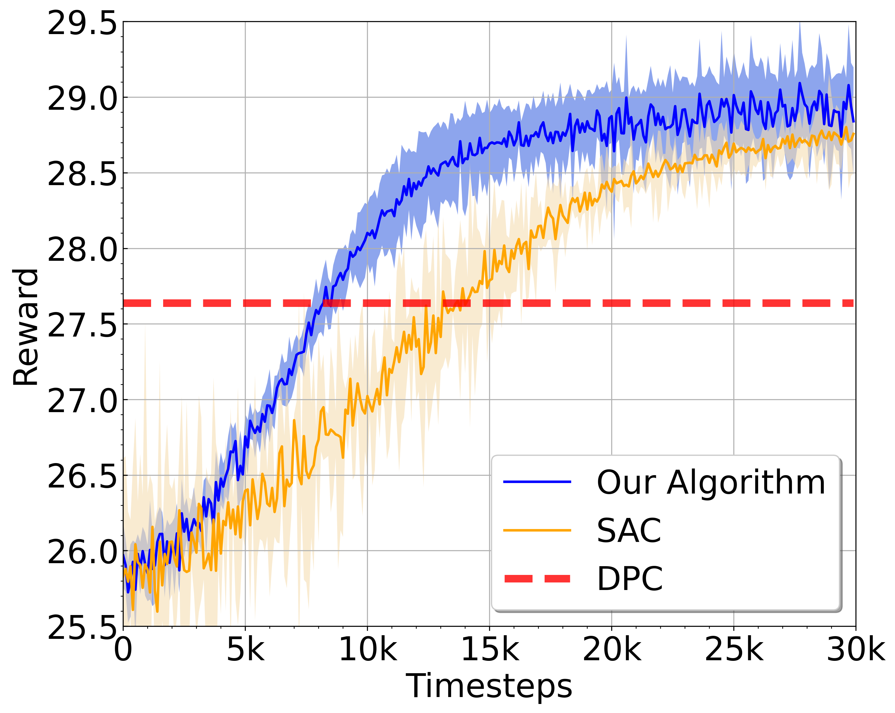
Distributed power control in wireless network: We considered the reward/utility of each agent is the difference between a logarithmic function of signal-interference-noise ratio (SINR) and a linear pricing function proportional to the transmitted power as in (3). In the literature, the problem has been formulated as a linear pricing game [2] and [5]. We compared Algorithm 2 with the DPC algorithm [2] and SAC in [20]. In our experiment, we first studied a setting with 66-link (3×23\times 2 grids) where the tabular method is tractable to represent value functions. Then we studied two settings: 99-link and 2525-link as shown in the right-hand side of Figure 2, where we use blue circles to denote links. For both settings, we use neural network (NN) approximation for value functions. With NN approximation, we utilized the replay buffer [17] and double-Q learning [11] to stabilize the learning process.

For the reward/utility in (3), we set Gn,n=1G_{n,n}=1 and Gm,n=κ/(distm,n)2G_{m,n}=\kappa/({dist}_{m,n})^{2} with κ=0.1\kappa=0.1 as the fading factor and distm,n{dist}_{m,n} is the distance between nodes mm and n.n. The average power of the noise is σn=0.1.\sigma_{n}=0.1. We set the trade-off parameter un=0.1,n.u_{n}=0.1,\forall n. For each environment, we ran 99 different instances with different random seeds and the shaded region represents the 95%95\% confidence interval.

For 66-nodes network, we represent value functions with tables in Algorithm 2. We observe the learning processes are quite stable in Figure 4(a). We observe our algorithm outperforms the SAC and DPC algorithm as the training time increases: the converged reward are (17.6017.60 v.s. 17.4317.43 v.s. 16.7716.77). For 9-nodes , we approximate value functions with neural networks in Algorithm 2. We observe Algorithm 2 outperforms the SAC and DPC algorithms as the training time increases in Figure 4(b) (28.9228.92 v.s. 28.7628.76 v.s. 27.6427.64). For 25 nodes, Figure 4(c) shows the results with a heterogeneous topology. Again, we observe our algorithm increases steady in Figure 4(c) and outperforms the SAC and DPC algorithms (98.3598.35 v.s. 95.7095.70 v.s. 95.3495.34).

Finally, we note that both ALOHA and DPC algorithms are model-based algorithm and the agents need to know the systems parameters (success transmitting probability in the real-time access control problem and channel gains and interference levels in the power control problem) while our algorithm is model-free and does not need to know these parameters.

6 Conclusion

In this paper, we studied a weakly-coupled multi-agent reinforcement learning problem where agents’ reward functions are coupled but the transition kernels are not. We propose TD-learning based regularized multi-agent policy actor-critic algorithm (TD-RDAC) that achieve the local convergence result. We demonstrated the effectiveness of TD-RDAC with two important applications in wireless networks: real-time access control and distributed power control and showed that our algorithm outperforms the existing benchmarks in the literature.

Acknowledgements

The authors are very grateful to Rui Hu for his insightful discussion and comments.

References

  • [1] Alekh Agarwal, Sham M Kakade, Jason D Lee, and Gaurav Mahajan. Optimality and approximation with policy gradient methods in markov decision processes. In Proceedings of Thirty Third Conference on Learning Theory, 2020.
  • [2] Tansu Alpcan, Tamer Başar, R. Srikant, and Eitan Altman. CDMA uplink power control as a non-cooperative game. Proceedings of the IEEE Conference on Decision and Control, 2001.
  • [3] Xingyan Chen, Changqiao Xu, Mu Wang, Zhonghui Wu, Shujie Yang, Lujie Zhong, and Gabriel-Miro Muntean. A universal transcoding and transmission method for livecast with networked multi-agent reinforcement learning. In IEEE Conference on Computer Communications, 2021.
  • [4] Ziyi Chen, Yi Zhou, Rong-Rong Chen, and Shaofeng Zou. Sample and communication-efficient decentralized actor-critic algorithms with finite-time analysis. In Proceedings of the 39th International Conference on Machine Learning, 2022.
  • [5] Mung Chiang, Prashanth Hande, Tian Lan, and Chee Wei Tan. Power control in wireless cellular networks. Foundations and Trends® in Networking, 2008.
  • [6] Tianshu Chu, Sandeep Chinchali, and Sachin Katti. Multi-agent reinforcement learning for networked system control. In International Conference on Learning Representations, 2020.
  • [7] Romuald Elie, Pérolat Julien, Mathieu Laurière, Matthieu Geist, and Olivier Pietquin. On the convergence of model free learning in mean field games. AAAI Conference on Artificial Intelligence, 2020.
  • [8] Jakob Foerster, Gregory Farquhar, Triantafyllos Afouras, Nantas Nardelli, and Shimon Whiteson. Counterfactual multi-agent policy gradients. AAAI Conference on Artificial Intelligence, 2018.
  • [9] Xin Guo, Anran Hu, Renyuan Xu, and Junzi Zhang. Learning mean-field games. In Advances in Neural Information Processing Systems, 2019.
  • [10] FNU Hairi, Jia Liu, and Songtao Lu. Finite-time convergence and sample complexity of multi-agent actor-critic reinforcement learning with average reward. In The Tenth International Conference on Learning Representations, 2022.
  • [11] Hado van Hasselt, Arthur Guez, and David Silver. Deep reinforcement learning with double q-learning. In Proceedings of the Thirtieth AAAI Conference on Artificial Intelligence, 2016.
  • [12] Vijay Konda and John Tsitsiklis. Actor-critic algorithms. In S. Solla, T. Leen, and K. Müller, editors, Advances in Neural Information Processing Systems, volume 12. MIT Press, 2000.
  • [13] Yiheng Lin, Guannan Qu, Longbo Huang, and Adam Wierman. Multi-agent reinforcement learning in stochastic networked systems. In Advances in Neural Information Processing Systems, 2021.
  • [14] Ryan Lowe, Yi Wu, Aviv Tamar, Jean Harb, Pieter Abbeel, and Igor Mordatch. Multi-agent actor-critic for mixed cooperative-competitive environments. In Proceedings of the 31st International Conference on Neural Information Processing Systems, 2017.
  • [15] Jincheng Mei, Chenjun Xiao, Csaba Szepesvari, and Dale Schuurmans. On the global convergence rates of softmax policy gradient methods. In Proceedings of the 37th International Conference on Machine Learning, 2020.
  • [16] Nicolas Meuleau, Milos Hauskrecht, Kee-Eung Kim, Leonid Peshkin, Leslie Pack Kaelbling, Thomas Dean, and Craig Boutilier. Solving very large weakly coupled markov decision processes. American Association for Artificial Intelligence, 1998.
  • [17] Volodymyr Mnih, Koray Kavukcuoglu, David Silver, Alex Graves, Ioannis Antonoglou, Daan Wierstra, and Martin Riedmiller. Playing atari with deep reinforcement learning. In International Conference on Neural Information Processing Systems, 2013.
  • [18] Guannan Qu, Yiheng Lin, Adam Wierman, and Na Li. Scalable multi-agent reinforcement learning for networked systems with average reward. arXiv preprint arXiv:2006.06626, 2020.
  • [19] Guannan Qu, Adam Wierman, and Na Li. Scalable reinforcement learning of localized policies for multi-agent networked systems. In Proceedings of the 2nd Conference on Learning for Dynamics and Control, 2020.
  • [20] Guannan Qu, Adam Wierman, and Na Li. Scalable reinforcement learning for multiagent networked systems. Operations Research, 2022.
  • [21] Lawrence G. Roberts. Aloha packet system with and without slots and capture. SIGCOMM Comput. Commun. Rev., 1975.
  • [22] R. Srikant and Lei Ying. Finite-time error bounds for linear stochastic approximation and TD learning. In Proceedings of the 22nd Annual Conference on Learning Theory (COLT), 2019.
  • [23] Shan Sun, Mariam Kiran, and Wei Ren. MAMRL: Exploiting multi-agent meta reinforcement learning in WAN traffic engineering. arXiv preprint arXiv:2111.15087, 2021.
  • [24] Richard S. Sutton, David McAllester, Satinder Singh, and Yishay Mansour. Policy gradient methods for reinforcement learning with function approximation. In Proceedings of the 12th International Conference on Neural Information Processing Systems, 1999.
  • [25] Fangxin Wang, Feng Wang, Jiangchuan Liu, Ryan Shea, and Lifeng Sun. Intelligent video caching at network edge: A multi-agent deep reinforcement learning approach. In IEEE Conference on Computer Communications, 2020.
  • [26] Xiaohan Wei, Hao Yu, and Michael J. Neely. Online learning in weakly coupled markov decision processes: A convergence time study. Proc. ACM Meas. Anal. Comput. Syst., apr 2018.
  • [27] Qiaomin Xie, Zhuoran Yang, Zhaoran Wang, and Andreea Minca. Learning while playing in mean-field games: Convergence and optimality. In Proceedings of the 38th International Conference on Machine Learning, 2021.
  • [28] Junzi Zhang, Jongho Kim, Brendan O’Donoghue, and Stephen Boyd. Sample efficient reinforcement learning with reinforce. In Proceedings of the AAAI Conference on Artificial Intelligence, 2021.
  • [29] Kaiqing Zhang, Zhuoran Yang, Han Liu, Tong Zhang, and Tamer Basar. Fully decentralized multi-agent reinforcement learning with networked agents. In Proceedings of the 35th International Conference on Machine Learning, 2018.
  • [30] Runyu Zhang, Zhaolin Ren, and Na Li. Gradient play in multi-agent markov stochastic games: Stationary points and convergence. arXiv preprint arXiv:2106.00198, 2021.
  • [31] Yizhou Zhang, Guannan Qu, Pan Xu, Yiheng Lin, Zaiwei Chen, and Adam Wierman. Global convergence of localized policy iteration in networked multi-agent reinforcement learning. arXiv preprint arXiv:2211.17116, 11 2022.

Appendix A Decomposition of Value Functions

A.1 Proof of Lemma 1

Proof 1

We provide the proof of the decomposition on QQ-function and the similar argument holds for the value function Vπθ(s).V^{\pi_{\theta}}(s). According to the definitions of reward and QQ-function, we have

Qπθ(s,a)=\displaystyle Q^{\pi_{\theta}}(s,a)= 1Nn=1N𝔼[t=1γtrn(s𝒩(n)t,a𝒩(n)t)|s0=s,a0=a]\displaystyle\frac{1}{N}\sum_{n=1}^{N}\mathbb{E}\left[\sum_{t=1}^{\infty}\gamma^{t}r_{n}(s_{\mathcal{N}(n)}^{t},a_{\mathcal{N}(n)}^{t})\Big{|}s^{0}=s,a^{0}=a\right]
=\displaystyle= 1Nn=1N𝔼[t=1γtrn(s𝒩(n)t,a𝒩(n)t)|s𝒩(n)0=s𝒩(n),a𝒩(n)0=a𝒩(n)]\displaystyle\frac{1}{N}\sum_{n=1}^{N}\mathbb{E}\left[\sum_{t=1}^{\infty}\gamma^{t}r_{n}(s_{\mathcal{N}(n)}^{t},a_{\mathcal{N}(n)}^{t})\Big{|}s_{\mathcal{N}(n)}^{0}=s_{\mathcal{N}(n)},a_{\mathcal{N}(n)}^{0}=a_{\mathcal{N}(n)}\right]
=\displaystyle= 1Nn=1NQnπθ(s𝒩(n),a𝒩(n))\displaystyle\frac{1}{N}\sum_{n=1}^{N}Q^{\pi_{\theta}}_{n}(s_{\mathcal{N}(n)},a_{\mathcal{N}(n)})

where the second equality holds because the reward and transition of agent nn only depends on its neighbors’ states and actions since for any trajectories of agent nn until t,t^{\prime}, we have

𝒫(s0,a0,,s𝒩(n)t,a𝒩(n)t)\displaystyle\mathcal{P}(s^{0},a^{0},\cdots,s_{\mathcal{N}(n)}^{t^{\prime}},a_{\mathcal{N}(n)}^{t^{\prime}}) =t=1tk𝒩(n)πθk(akt|skt)𝒫(skt|skt1,akt1)\displaystyle=\prod_{t=1}^{t^{\prime}}\prod_{k\in\mathcal{N}(n)}{\pi_{\theta_{k}}(a_{k}^{t}|s_{k}^{t})\mathcal{P}(s_{k}^{t}|s_{k}^{t-1},a_{k}^{t-1})}
=k𝒩(n)t=1tπθk(akt|skt)𝒫(skt|skt1,akt1)\displaystyle=\prod_{k\in\mathcal{N}(n)}\prod_{t=1}^{t^{\prime}}{\pi_{\theta_{k}}(a_{k}^{t}|s_{k}^{t})\mathcal{P}(s_{k}^{t}|s_{k}^{t-1},a_{k}^{t-1})}
=𝒫(s𝒩(n)0,a𝒩(n)0,,s𝒩(n)t,a𝒩(n)t),\displaystyle=\mathcal{P}(s_{\mathcal{N}(n)}^{0},a_{\mathcal{N}(n)}^{0},\cdots,s_{\mathcal{N}(n)}^{t^{\prime}},a_{\mathcal{N}(n)}^{t^{\prime}}),

and it implies 𝒫(s𝒩(n)t,a𝒩(n)t)\mathcal{P}(s_{\mathcal{N}(n)}^{t^{\prime}},a_{\mathcal{N}(n)}^{t^{\prime}}) only depends on (s𝒩(n)0,a𝒩(n)0).(s_{\mathcal{N}(n)}^{0},a_{\mathcal{N}(n)}^{0}).

A.2 Proof of Lemma 2

Proof 2

According to Theorem 1, we have

θnVπθ(ρ)=\displaystyle\nabla_{\theta_{n}}V^{\pi_{\theta}}(\rho)= 11γ𝔼sdρπθ,aπθ(|s)[Qπθ(s,a)θnlogπθ(a|s)]\displaystyle\frac{1}{1-\gamma}\mathbb{E}_{s\sim d^{\pi_{\theta}}_{\rho},a\sim\pi_{\theta}(\cdot|s)}\left[Q^{\pi_{\theta}}(s,a)\nabla_{\theta_{n}}\log\pi_{\theta}(a|s)\right]
=\displaystyle= 11γ𝔼sdρπθ,aπθ(|s)[Qπθ(s,a)θnlogπθn(an|sn)]\displaystyle\frac{1}{1-\gamma}\mathbb{E}_{s\sim d^{\pi_{\theta}}_{\rho},a\sim\pi_{\theta}(\cdot|s)}\left[Q^{\pi_{\theta}}(s,a)\nabla_{\theta_{n}}\log\pi_{\theta_{n}}(a_{n}|s_{n})\right]
=\displaystyle= 11γ𝔼sdρπθ,aπθ(|s)[1Nn=1NQπθ(s𝒩(n),a𝒩(n))θnlogπθn(an|sn)]\displaystyle\frac{1}{1-\gamma}\mathbb{E}_{s\sim d^{\pi_{\theta}}_{\rho},a\sim\pi_{\theta}(\cdot|s)}\left[\frac{1}{N}\sum_{n=1}^{N}Q^{\pi_{\theta}}(s_{\mathcal{N}(n)},a_{\mathcal{N}(n)})\nabla_{\theta_{n}}\log\pi_{\theta_{n}}(a_{n}|s_{n})\right]
=\displaystyle= 11γ𝔼sdρπθ,aπθ(|s)[1Nk𝒩(n)Qπθ(s𝒩(k),a𝒩(k))θnlogπθn(an|sn)]\displaystyle\frac{1}{1-\gamma}\mathbb{E}_{s\sim d^{\pi_{\theta}}_{\rho},a\sim\pi_{\theta}(\cdot|s)}\left[\frac{1}{N}\sum_{k\in\mathcal{N}(n)}Q^{\pi_{\theta}}(s_{\mathcal{N}(k)},a_{\mathcal{N}(k)})\nabla_{\theta_{n}}\log\pi_{\theta_{n}}(a_{n}|s_{n})\right]

where the second equality holds because of localized policies πθ(a|s)=nπθn(an|sn);\pi_{\theta}(a|s)=\prod_{n}\pi_{\theta_{n}}(a_{n}|s_{n}); the third equality holds because of Lemma 1; the last equality holds because for any k𝒩(n)k\notin\mathcal{N}(n) that

𝔼sdρπθ,aπθ(|s)[Qπθ(s𝒩(k),a𝒩(k))θnlogπθn(an|sn)]\displaystyle\mathbb{E}_{s\sim d^{\pi_{\theta}}_{\rho},a\sim\pi_{\theta}(\cdot|s)}\left[Q^{\pi_{\theta}}(s_{\mathcal{N}(k)},a_{\mathcal{N}(k)})\nabla_{\theta_{n}}\log\pi_{\theta_{n}}(a_{n}|s_{n})\right]
=\displaystyle= 𝔼sdρπθ[aQπθ(s𝒩(k),a𝒩(k))jnπθj(aj|sj)θnπθn(an|sn)]\displaystyle\mathbb{E}_{s\sim d^{\pi_{\theta}}_{\rho}}\left[\sum_{a}Q^{\pi_{\theta}}(s_{\mathcal{N}(k)},a_{\mathcal{N}(k)})\prod_{j\neq n}\pi_{\theta_{j}}(a_{j}|s_{j})\nabla_{\theta_{n}}\pi_{\theta_{n}}(a_{n}|s_{n})\right]
=\displaystyle= 𝔼sdρπθ[anQπθ(s𝒩(k),a𝒩(k))jnπθj(aj|sj)anθnπθn(an|sn)]\displaystyle\mathbb{E}_{s\sim d^{\pi_{\theta}}_{\rho}}\left[\sum_{a_{-n}}Q^{\pi_{\theta}}(s_{\mathcal{N}(k)},a_{\mathcal{N}(k)})\prod_{j\neq n}\pi_{\theta_{j}}(a_{j}|s_{j})\sum_{a_{n}}\nabla_{\theta_{n}}\pi_{\theta_{n}}(a_{n}|s_{n})\right]
=\displaystyle= 0\displaystyle 0

Note θnVπθ(ρ)=11γ𝔼sdρπθ,aπθ(|s)[Aπθ(s,a)θnlogπθ(a|s)]\nabla_{\theta_{n}}V^{\pi_{\theta}}(\rho)=\frac{1}{1-\gamma}\mathbb{E}_{s\sim d^{\pi_{\theta}}_{\rho},a\sim\pi_{\theta}(\cdot|s)}\left[A^{\pi_{\theta}}(s,a)\nabla_{\theta_{n}}\log\pi_{\theta}(a|s)\right] and the second equality on the advantage function holds by following the same steps.

Appendix B Proof of Theorem 2

To prove Theorem 2, we first prove the smoothness of regularized value LL function.

B.1 Smoothness of LL function

Recall the definition of LL function

Lλ(θ)=Vπθ(ρ)+R(θ).L_{\lambda}(\theta)=V^{\pi_{\theta}}(\rho)+R(\theta).

where R(θ)=n=1Nλ|𝒮n||𝒜n|sn,anlogπθn(an|sn).R(\theta)=\sum_{n=1}^{N}\frac{\lambda}{|\mathcal{S}_{n}||\mathcal{A}_{n}|}\sum_{s_{n},a_{n}}\log\pi_{\theta_{n}}(a_{n}|s_{n}). We show Vπθ(ρ)V^{\pi_{\theta}}(\rho) is 48N2(1γ)3\frac{48N^{2}}{(1-\gamma)^{3}}-smoothness in Lemma 3 and R(θ)R(\theta) is n2λ|𝒮n|\sum_{n}\frac{2\lambda}{|\mathcal{S}_{n}|}-smoothness in Lemma 4, respectively, which imply Lπθ(s)L^{\pi_{\theta}}(s) is β:=48N2(1γ)3+n2λ|𝒮n|\beta^{\prime}:=\frac{48N^{2}}{(1-\gamma)^{3}}+\sum_{n}\frac{2\lambda}{|\mathcal{S}_{n}|} smoothness.

Lemma 3 (Smoothness)

Under Algorithm 1, we have Vπθ(s)V^{\pi_{\theta}}(s) to be 48N2/(1γ)348N^{2}/(1-\gamma)^{3} smoothness, i.e.,

|Vπθ(s)Vπθ(s)Vπθ(s)θ,θθ|24N2(1γ)3θθ2.\left|V^{\pi_{\theta}}(s)-V^{\pi_{\theta^{\prime}}}(s)-\langle\frac{\partial V^{\pi_{\theta}}(s)}{\partial\theta},\theta-\theta^{\prime}\rangle\right|\leq\frac{24N^{2}}{(1-\gamma)^{3}}||\theta-\theta^{\prime}||^{2}.
Proof 3

The Bellman equation (for a network) is

Vπθ(s)=aπθ(a|s)r(s,a)+γaπθ(a|s)s𝒫(s|s,a)Vπθ(s),V^{\pi_{\theta}}(s)=\sum_{a}\pi_{\theta}(a|s)r(s,a)+\gamma\sum_{a}\pi_{\theta}(a|s)\sum_{s^{\prime}}\mathcal{P}(s^{\prime}|s,a)V^{\pi_{\theta}}(s^{\prime}),

Let

rθ(s)=aπ(a|s)r(s,a)and𝒫θ(s,s)=aπθ(a|s)s𝒫(s|s,a).r_{\theta}(s)=\sum_{a}\pi(a|s)r(s,a)~{}~{}\text{and}~{}~{}\mathcal{P}_{\theta}(s,s^{\prime})=\sum_{a}\pi_{\theta}(a|s)\sum_{s^{\prime}}\mathcal{P}(s^{\prime}|s,a).

Let usu_{s} be a vector with only the ssth entry being one and zeros for other entries. The Bellman equation can be wrote as

Vπθ(s)=\displaystyle V^{\pi_{\theta}}(s)= rθ(s)+γ𝒫θ(s,),Vπθ(),\displaystyle r_{\theta}(s)+\gamma\langle\mathcal{P}_{\theta}(s,\cdot),V^{\pi_{\theta}}(\cdot)\rangle,

which implies Vπθ|𝒮|V^{\pi_{\theta}}\in\mathbb{R}^{|\mathcal{S}|} satisfies

Vπθ=(Iγ𝒫(θ))1rθ:=Mθrθ,V^{\pi_{\theta}}=(I-\gamma\mathcal{P}(\theta))^{-1}r_{\theta}:=M_{\theta}r_{\theta},

where II is the identity matrix. Let θα=θ+αν,\theta_{\alpha}=\theta+\alpha\nu, and we have ν2Vπθ(s)θ2ν=2Vπθα(s)α2|α=0.\nu^{\dagger}\frac{\partial^{2}V^{\pi_{\theta}}(s)}{\partial\theta^{2}}\nu=\frac{\partial^{2}V^{\pi_{\theta_{\alpha}}}(s)}{\partial\alpha^{2}}|_{\alpha=0}. With a bit abuse of notation, let rα=rθα,r_{\alpha}=r_{\theta_{\alpha}}, 𝒫α=𝒫θα,\mathcal{P}_{\alpha}=\mathcal{P}_{\theta_{\alpha}}, πα=πθα,\pi_{\alpha}=\pi_{\theta_{\alpha}}, and Mα=Mθα.M_{\alpha}=M_{\theta_{\alpha}}. We need to compute the first-order gradient

Vπθα(s)α=\displaystyle\frac{\partial V^{\pi_{\theta_{\alpha}}}(s)}{\partial\alpha}= γusTMααrα+usTMαrαα\displaystyle\gamma u_{s}^{T}\frac{\partial M_{\alpha}}{\partial\alpha}r_{\alpha}+u_{s}^{T}M_{\alpha}\frac{\partial r_{\alpha}}{\partial\alpha}
=\displaystyle= γusTMα𝒫ααMαrα+usTMαrαα\displaystyle\gamma u_{s}^{T}M_{\alpha}\frac{\partial\mathcal{P}_{\alpha}}{\partial\alpha}M_{\alpha}r_{\alpha}+u_{s}^{T}M_{\alpha}\frac{\partial r_{\alpha}}{\partial\alpha}

where we use the derivative of inverse matrix (Iγ𝒫(θ))1α=(Iγ𝒫(θ))1(Iγ𝒫(θ))α(Iγ𝒫(θ))1;\frac{\partial(I-\gamma\mathcal{P}(\theta))^{-1}}{\partial\alpha}=(I-\gamma\mathcal{P}(\theta))^{-1}\frac{\partial(I-\gamma\mathcal{P}(\theta))}{\partial\alpha}(I-\gamma\mathcal{P}(\theta))^{-1}; and the second-order gradient

2Vπθα(s)α2=\displaystyle\frac{\partial^{2}V^{\pi_{\theta_{\alpha}}}(s)}{\partial\alpha^{2}}= 2γ2usTMα𝒫ααMα𝒫ααMαrα+γusTMα2𝒫αα2Mαrα\displaystyle 2\gamma^{2}u_{s}^{T}M_{\alpha}\frac{\partial\mathcal{P}_{\alpha}}{\partial\alpha}M_{\alpha}\frac{\partial\mathcal{P}_{\alpha}}{\partial\alpha}M_{\alpha}r_{\alpha}+\gamma u_{s}^{T}M_{\alpha}\frac{\partial^{2}\mathcal{P}_{\alpha}}{\partial\alpha^{2}}M_{\alpha}r_{\alpha}
+γusTMα𝒫ααMαrαα+usTMα2rαα2.\displaystyle+\gamma u_{s}^{T}M_{\alpha}\frac{\partial\mathcal{P}_{\alpha}}{\partial\alpha}M_{\alpha}\frac{\partial r_{\alpha}}{\partial\alpha}+u_{s}^{T}M_{\alpha}\frac{\partial^{2}r_{\alpha}}{\partial\alpha^{2}}.

Therefore, we need to establish the upper bounds on

𝒫αα,2𝒫αα2,rαα,2rαα2,\frac{\partial\mathcal{P}_{\alpha}}{\partial\alpha},~{}~{}\frac{\partial^{2}\mathcal{P}_{\alpha}}{\partial\alpha^{2}},~{}~{}\frac{\partial r_{\alpha}}{\partial\alpha},~{}~{}\frac{\partial^{2}r_{\alpha}}{\partial\alpha^{2}},

which require to compute

παα,2παα2.\frac{\partial\pi_{\alpha}}{\partial\alpha},~{}~{}\frac{\partial^{2}\pi_{\alpha}}{\partial\alpha^{2}}.

Recall πθ(a|s)=n=1Nπθn(an|sn).\pi_{\theta}(a|s)=\prod_{n=1}^{N}\pi_{\theta_{n}}(a_{n}|s_{n}). Let’s compute

πα(a|s)α|α=0\displaystyle\frac{\partial\pi_{\alpha}(a|s)}{\partial\alpha}|_{\alpha=0} =πθ(a|s)θ(s,),ν(s,)=n=1Nπθ(a|s)θn(sn,),νn(sn,)\displaystyle=\langle\frac{\partial\pi_{\theta}(a|s)}{\partial\theta(s,\cdot)},\nu(s,\cdot)\rangle=\sum_{n=1}^{N}\langle\frac{\partial\pi_{\theta}(a|s)}{\partial\theta_{n}(s_{n},\cdot)},\nu_{n}(s_{n},\cdot)\rangle
=n=1Nknπθk(ak|sk)πθn(an|sn)θn(sn,),νn(sn,)\displaystyle=\sum_{n=1}^{N}\prod_{k\neq n}\pi_{\theta_{k}}(a_{k}|s_{k})~{}\langle\frac{\partial\pi_{\theta_{n}}(a_{n}|s_{n})}{\partial\theta_{n}(s_{n},\cdot)},\nu_{n}(s_{n},\cdot)\rangle
=n=1Nπθ(a|s)(νn(sn,an)πθn(|sn),νn(s,))\displaystyle=\sum_{n=1}^{N}\pi_{\theta}(a|s)\left(\nu_{n}(s_{n},a_{n})-\langle\pi_{\theta_{n}}(\cdot|s_{n}),\nu_{n}(s,\cdot)\rangle\right)

where the last equality holds because

πθn(an|sn)θn(sn,an)=πθn(an|sn)(𝕀an=anπθn(an|sn)),\frac{\partial\pi_{\theta_{n}}(a_{n}|s_{n})}{\partial\theta_{n}(s_{n},a^{\prime}_{n})}=\pi_{\theta_{n}}(a_{n}|s_{n})(\mathbb{I}_{a_{n}=a^{\prime}_{n}}-\pi_{\theta_{n}}(a^{\prime}_{n}|s_{n})),

and it implies

πθn(an|sn)θn(sn,),νn(sn,)=νn(sn,an)πθn(|sn),νn(s,).\langle\frac{\partial\pi_{\theta_{n}}(a_{n}|s_{n})}{\partial\theta_{n}(s_{n},\cdot)},\nu_{n}(s_{n},\cdot)\rangle=\nu_{n}(s_{n},a_{n})-\langle\pi_{\theta_{n}}(\cdot|s_{n}),\nu_{n}(s,\cdot)\rangle.

Therefore, we have

a|πα(a|s)α|α=0|\displaystyle\sum_{a}\left|\frac{\partial\pi_{\alpha}(a|s)}{\partial\alpha}|_{\alpha=0}\right| =a|n=1Nπθ(a|s)(νn(sn,an)πθn(|sn),νn(sn,))|\displaystyle=\sum_{a}\left|\sum_{n=1}^{N}\pi_{\theta}(a|s)\left(\nu_{n}(s_{n},a_{n})-\langle\pi_{\theta_{n}}(\cdot|s_{n}),\nu_{n}(s_{n},\cdot)\rangle\right)\right|
2maxan=1N|νn(sn,an)|\displaystyle\leq 2\max_{a}\sum_{n=1}^{N}|\nu_{n}(s_{n},a_{n})|
2Nu2.\displaystyle\leq 2N||u||_{2}.

Next, let’s compute

2πα(a|s)α2|α=0\displaystyle\frac{\partial^{2}\pi_{\alpha}(a|s)}{\partial\alpha^{2}}|_{\alpha=0} =n=1Nn=1N2πθ(a|s)θn(sn,)θn(sn,)νn(sn,),νn(sn,),\displaystyle=\sum_{n=1}^{N}\sum_{n^{\prime}=1}^{N}\langle\frac{\partial^{2}\pi_{\theta}(a|s)}{\partial\theta_{n}(s_{n},\cdot)\theta_{n^{\prime}}(s_{n^{\prime}},\cdot)}\nu_{n}(s_{n},\cdot),\nu_{n^{\prime}}(s_{n^{\prime}},\cdot)\rangle,

where we need to compute

(2πθ(a|s)θn(sn,)2)i,j=\displaystyle\left(\frac{\partial^{2}\pi_{\theta}(a|s)}{\partial\theta_{n}(s_{n},\cdot)^{2}}\right)_{i,j}= 𝕀an=iπθ(a|s)(𝕀an=jπθn(j|sn))πθ(a|s)πθn(i|sn)(𝕀i=jπθn(j|sn))\displaystyle\mathbb{I}_{a_{n}=i}\pi_{\theta}(a|s)\left(\mathbb{I}_{a_{n}=j}-\pi_{\theta_{n}}(j|s_{n})\right)-\pi_{\theta}(a|s)\pi_{\theta_{n}}(i|s_{n})\left(\mathbb{I}_{i=j}-\pi_{\theta_{n}}(j|s_{n})\right)
πθ(a|s)πθn(i|sn)(𝕀an=jπθn(j|sn)),\displaystyle-\pi_{\theta}(a|s)\pi_{\theta_{n}}(i|s_{n})\left(\mathbb{I}_{a_{n}=j}-\pi_{\theta_{n}}(j|s_{n})\right),

and

(2πθ(a|s)θn(sn,)θn(sn,))i,j=\displaystyle\left(\frac{\partial^{2}\pi_{\theta}(a|s)}{\partial\theta_{n}(s_{n},\cdot)\theta_{n^{\prime}}(s_{n^{\prime}},\cdot)}\right)_{i,j}= πθ(a|s)(𝕀an=iπθn(i|sn))(𝕀an=jπθn(j|sn)).\displaystyle\pi_{\theta}(a|s)\left(\mathbb{I}_{a_{n}=i}-\pi_{\theta_{n}}(i|s_{n})\right)\left(\mathbb{I}_{a_{n^{\prime}}=j}-\pi_{\theta_{n^{\prime}}}(j|s_{n^{\prime}})\right).

Then we have

|2πθ(a|s)θn(sn,)2νn(sn,),νn(sn,)/π(a|s)|\displaystyle\left|\langle\frac{\partial^{2}\pi_{\theta}(a|s)}{\partial\theta_{n}(s_{n},\cdot)^{2}}\nu_{n}(s_{n},\cdot),\nu_{n}(s_{n},\cdot)\rangle/\pi(a|s)\right|
\displaystyle\leq νn2(sn,an)+2|νn(sn,an)jπθn(j|sn)νn(sn,j)|\displaystyle\nu^{2}_{n}(s_{n},a_{n})+2|\nu_{n}(s_{n},a_{n})\sum_{j}\pi_{\theta_{n}}(j|s_{n})\nu_{n}(s_{n},j)|
+|iπθn(i|s)νn2(i|s)+2ijπθn(i|sn)πθn(j|sn)νn(sn,i)νn(sn,j)|\displaystyle+|\sum_{i}\pi_{\theta_{n}}(i|s)\nu^{2}_{n}(i|s)+2\sum_{i}\sum_{j}\pi_{\theta_{n}}(i|s_{n})\pi_{\theta_{n}}(j|s_{n})\nu_{n}(s_{n},i)\nu_{n^{\prime}}(s_{n^{\prime}},j)|
\displaystyle\leq 6maxanνn2(sn,an),\displaystyle 6\max_{a_{n}}\nu^{2}_{n}(s_{n},a_{n}),

and

|2πθ(a|s)θn(sn,)θn(sn,)νn(sn,),νn(sn,)/π(a|s)|\displaystyle\left|\langle\frac{\partial^{2}\pi_{\theta}(a|s)}{\partial\theta_{n}(s_{n},\cdot)\theta_{n^{\prime}}(s_{n^{\prime}},\cdot)}\nu_{n}(s_{n},\cdot),\nu_{n^{\prime}}(s_{n^{\prime}},\cdot)\rangle/\pi(a|s)\right|
\displaystyle\leq |νn(sn,an)νn(sn,an)|+|νn(sn,an)jπθn(j|sn)νn(sn,j)|\displaystyle|\nu_{n}(s_{n},a_{n})\nu_{n^{\prime}}(s_{n^{\prime}},a_{n^{\prime}})|+|\nu_{n}(s_{n},a_{n})\sum_{j}\pi_{\theta_{n^{\prime}}}(j|s_{n^{\prime}})\nu_{n^{\prime}}(s_{n^{\prime}},j)| (4)
+|νn(sn,an)iπθn(i|sn)νn(sn,i)|+ij|πθn(i|sn)πθn(j|sn)νn(sn,i)νn(sn,j)|\displaystyle+|\nu_{n^{\prime}}(s_{n^{\prime}},a_{n^{\prime}})\sum_{i}\pi_{\theta_{n}}(i|s_{n})\nu_{n}(s_{n},i)|+\sum_{i}\sum_{j}|\pi_{\theta_{n}}(i|s_{n})\pi_{\theta_{n^{\prime}}}(j|s_{n^{\prime}})\nu_{n}(s_{n},i)\nu_{n^{\prime}}(s_{n^{\prime}},j)| (5)
\displaystyle\leq 4maxsn,sn,an,an|νn(sn,an)νn(sn,an)|\displaystyle 4\max_{s_{n},s_{n^{\prime}},a_{n},a_{n^{\prime}}}|\nu_{n}(s_{n},a_{n})\nu_{n^{\prime}}(s_{n^{\prime}},a_{n^{\prime}})| (6)

which implies

|2πα(a|s)α2|α=0|6N2||ν||22\displaystyle\left|\frac{\partial^{2}\pi_{\alpha}(a|s)}{\partial\alpha^{2}}|_{\alpha=0}\right|\leq 6N^{2}||\nu||_{2}^{2} (7)

Now it is good to bound

|2Vπθα(s)α2|α=0|=\displaystyle\left|\frac{\partial^{2}V^{\pi_{\theta_{\alpha}}}(s)}{\partial\alpha^{2}}|_{\alpha=0}\right|= 2γ2|usTMα𝒫ααMα𝒫ααMαrα|+γ|usTMα2𝒫αα2Mαrα|\displaystyle 2\gamma^{2}\left|u_{s}^{T}M_{\alpha}\frac{\partial\mathcal{P}_{\alpha}}{\partial\alpha}M_{\alpha}\frac{\partial\mathcal{P}_{\alpha}}{\partial\alpha}M_{\alpha}r_{\alpha}\right|+\gamma\left|u_{s}^{T}M_{\alpha}\frac{\partial^{2}\mathcal{P}_{\alpha}}{\partial\alpha^{2}}M_{\alpha}r_{\alpha}\right|
+γ|usTMα𝒫ααMαrαα|+|usTMα2rαα2|\displaystyle+\gamma\left|u_{s}^{T}M_{\alpha}\frac{\partial\mathcal{P}_{\alpha}}{\partial\alpha}M_{\alpha}\frac{\partial r_{\alpha}}{\partial\alpha}\right|+\left|u_{s}^{T}M_{\alpha}\frac{\partial^{2}r_{\alpha}}{\partial\alpha^{2}}\right|
\displaystyle\leq [8N2(1γ)3+6N2(1γ)2+4N2(1γ)2+6N2(1γ)2]ν22\displaystyle\left[\frac{8N^{2}}{(1-\gamma)^{3}}+\frac{6N^{2}}{(1-\gamma)^{2}}+\frac{4N^{2}}{(1-\gamma)^{2}}+\frac{6N^{2}}{(1-\gamma)^{2}}\right]||\nu||_{2}^{2}
\displaystyle\leq 24N2(1γ)3ν22.\displaystyle\frac{24N^{2}}{(1-\gamma)^{3}}||\nu||_{2}^{2}.

Finally, we have

ν2Vπθ(s)θ2ν24N2(1γ)3ν22,\nu^{\dagger}\frac{\partial^{2}V^{\pi_{\theta}}(s)}{\partial\theta^{2}}\nu\leq\frac{24N^{2}}{(1-\gamma)^{3}}||\nu||_{2}^{2},

which completes the proof.

Lemma 4

Under Algorithm 1, we have R(θ)R(\theta) is n2λ|𝒮n|\sum_{n}\frac{2\lambda}{|\mathcal{S}_{n}|}-smoothness.

Proof 4

We have for any nn such that

R(θ)θn(sn,)=\displaystyle\frac{\partial R(\theta)}{\partial\theta_{n}(s_{n},\cdot)}= 1|𝒮n|(1|𝒜n|πθn(|sn)),\displaystyle\frac{1}{|\mathcal{S}_{n}|}\left(\frac{1}{|\mathcal{A}_{n}|}-\pi_{\theta_{n}}(\cdot|s_{n})\right),
2R(θ)θn(sn,)2=\displaystyle\frac{\partial^{2}R(\theta)}{\partial\theta_{n}(s_{n},\cdot)^{2}}= 1|𝒮n|(diag(πθn(|sn))+πθn(|sn)πθn(|sn)T),\displaystyle\frac{1}{|\mathcal{S}_{n}|}\left(-\text{diag}(\pi_{\theta_{n}}(\cdot|s_{n}))+\pi_{\theta_{n}}(\cdot|s_{n})\pi_{\theta_{n}}(\cdot|s_{n})^{T}\right),

which implies

2R(θ)θn(sn,)2νn(sn,),νn(sn,)\displaystyle\langle\frac{\partial^{2}R(\theta)}{\partial\theta_{n}(s_{n},\cdot)^{2}}\nu_{n}(s_{n},\cdot),\nu_{n}(s_{n},\cdot)\rangle\leq |diag(πθn(|sn))νn(sn,),νn(sn,)|+πθn(|sn),νn(sn,)2\displaystyle\left|\langle\text{diag}(\pi_{\theta_{n}}(\cdot|s_{n}))\nu_{n}(s_{n},\cdot),\nu_{n}(s_{n},\cdot)\rangle\right|+\|\langle\pi_{\theta_{n}}(\cdot|s_{n}),\nu_{n}(s_{n},\cdot)\rangle\|^{2}
\displaystyle\leq 2νn(sn,)2.\displaystyle 2\|\nu_{n}(s_{n},\cdot)\|^{2}.

Finally we have

2R(θ)θ2ν,ν)2ν2,\langle\frac{\partial^{2}R(\theta)}{\partial\theta^{2}}\nu,\nu)\rangle\leq 2\|\nu\|^{2},

which completes the proof.

B.2 Proving Theorem 2

Recall η1/β\eta\leq 1/\beta^{\prime} and D(t)=L(ρ)Lπθt(ρ).D(t)=L^{*}(\rho)-L^{\pi_{\theta^{t}}}(\rho). Given θt\theta^{t} and L^πθt(ρ),\nabla\hat{L}^{\pi_{\theta^{t}}}(\rho), we have

D(t+1)D(t)=\displaystyle D(t+1)-D(t)= Lπθt(ρ)Lπθt+1(ρ)\displaystyle L^{\pi_{\theta^{t}}}(\rho)-L^{\pi_{\theta^{t+1}}}(\rho)
=\displaystyle= Lπθt(ρ)Lπθt+1(ρ)+Lπθt(ρ),θt+1θtLπθt(ρ),θt+1θt\displaystyle L^{\pi_{\theta^{t}}}(\rho)-L^{\pi_{\theta^{t+1}}}(\rho)+\langle\nabla L^{\pi_{\theta^{t}}}(\rho),\theta^{t+1}-\theta^{t}\rangle-\langle\nabla L^{\pi_{\theta^{t}}}(\rho),\theta^{t+1}-\theta^{t}\rangle
\displaystyle\leq β2θt+1θt2Lπθt(ρ),θt+1θt\displaystyle\frac{\beta^{\prime}}{2}||\theta^{t+1}-\theta^{t}||^{2}-\langle\nabla L^{\pi_{\theta^{t}}}(\rho),\theta^{t+1}-\theta^{t}\rangle
=\displaystyle= βη22L^πθt(ρ)2ηLπθt(ρ),L^πθt(ρ)\displaystyle\frac{\beta^{\prime}\eta^{2}}{2}||\nabla\hat{L}^{\pi_{\theta^{t}}}(\rho)||^{2}-\eta\langle\nabla L^{\pi_{\theta^{t}}}(\rho),\nabla\hat{L}^{\pi_{\theta^{t}}}(\rho)\rangle
=\displaystyle= 12βL^πθt(ρ)Lπθt(ρ)212βLπθt(ρ)2.\displaystyle\frac{1}{2\beta^{\prime}}||\nabla\hat{L}^{\pi_{\theta^{t}}}(\rho)-\nabla L^{\pi_{\theta^{t}}}(\rho)||^{2}-\frac{1}{2\beta}||\nabla L^{\pi_{\theta^{t}}}(\rho)||^{2}.

Since ϵt=𝔼[L^πθt(ρ)Lπθt(ρ)2],\epsilon_{t}=\mathbb{E}\left[||\nabla\hat{L}^{\pi_{\theta^{t}}}(\rho)-\nabla L^{\pi_{\theta^{t}}}(\rho)||^{2}\right], we have

𝔼[D(t+1)D(t)]\displaystyle\mathbb{E}\left[D(t+1)-D(t)\right]\leq 12β𝔼[L^πθt(ρ)Lπθt(ρ)2]12β𝔼[Lπθt(ρ)2],\displaystyle\frac{1}{2\beta^{\prime}}\mathbb{E}\left[||\nabla\hat{L}^{\pi_{\theta^{t}}}(\rho)-\nabla L^{\pi_{\theta^{t}}}(\rho)||^{2}\right]-\frac{1}{2\beta^{\prime}}\mathbb{E}\left[||\nabla L^{\pi_{\theta^{t}}}(\rho)||^{2}\right],

which implies

12β𝔼[Lπθt(ρ)2]\displaystyle\frac{1}{2\beta^{\prime}}\mathbb{E}\left[||\nabla L^{\pi_{\theta^{t}}}(\rho)||^{2}\right]\leq 12β𝔼[L^πθt(ρ)Lπθt(ρ)2]+𝔼[D(t)D(t+1)]\displaystyle\frac{1}{2\beta^{\prime}}\mathbb{E}\left[||\nabla\hat{L}^{\pi_{\theta^{t}}}(\rho)-\nabla L^{\pi_{\theta^{t}}}(\rho)||^{2}\right]+\mathbb{E}\left[D(t)-D(t+1)\right]
=\displaystyle= ϵt2β+𝔼[D(t)D(t+1)].\displaystyle\frac{\epsilon_{t}}{2\beta^{\prime}}+\mathbb{E}\left[D(t)-D(t+1)\right].

Take summation t=1,2,,Tt=1,2,\cdots,T and we have

t=1T𝔼[Lπθt(ρ)2]t=1Tϵt+2β(L(ρ)Lπ1(ρ)).\sum_{t=1}^{T}\mathbb{E}\left[||\nabla L^{\pi_{\theta^{t}}}(\rho)||^{2}\right]\leq\sum_{t=1}^{T}\epsilon_{t}+2\beta^{\prime}\left(L^{*}(\rho)-L^{\pi^{1}}(\rho)\right).

Appendix C Proof of Theorem 3

Recall the estimated gradient and the true gradient to be

θnV^πθ(ρ)=\displaystyle\nabla_{\theta_{n}}\hat{V}^{\pi_{\theta}}(\rho)= h=1Hγh1Nk𝒩(n)δ^kπθ,h(s𝒩(k)(h),a𝒩(k)(h))θnlogπθn(an(h)|sn(h)),\displaystyle\sum_{h=1}^{H}\gamma^{h}\frac{1}{N}\sum_{k\in\mathcal{N}(n)}\hat{\delta}^{\pi_{\theta},h}_{k}(s_{\mathcal{N}(k)}(h),a_{\mathcal{N}(k)}(h))\nabla_{\theta_{n}}\log\pi_{\theta_{n}}(a_{n}(h)|s_{n}(h)),
θnVπθ(ρ)=\displaystyle\nabla_{\theta_{n}}V^{\pi_{\theta}}(\rho)= h=1γh𝔼[1Nk𝒩(n)δkπθ,h(s𝒩(k)(h),a𝒩(k)(h))θnlogπθn(an(h)|sn(h))].\displaystyle\sum_{h=1}^{\infty}\gamma^{h}\mathbb{E}\left[\frac{1}{N}\sum_{k\in\mathcal{N}(n)}\delta^{\pi_{\theta},h}_{k}(s_{\mathcal{N}(k)}(h),a_{\mathcal{N}(k)}(h))\nabla_{\theta_{n}}\log\pi_{\theta_{n}}(a_{n}(h)|s_{n}(h))\right].

Further define θnV~πθ(ρ)\nabla_{\theta_{n}}\tilde{V}^{\pi_{\theta}}(\rho) and θnV~πθ(ρ)\nabla_{\theta_{n}}\tilde{V}^{\pi_{\theta}}(\rho) to decompose policy gradient as follows:

θnV~πθ(ρ)=\displaystyle\nabla_{\theta_{n}}\tilde{V}^{\pi_{\theta}}(\rho)= h=1Hγh1Nk𝒩(n)δkπθ,h(s𝒩(k)(h),a𝒩(k)(h))θnlogπθn(an(h)|sn(h)),\displaystyle\sum_{h=1}^{H}\gamma^{h}\frac{1}{N}\sum_{k\in\mathcal{N}(n)}\delta^{\pi_{\theta},h}_{k}(s_{\mathcal{N}(k)}(h),a_{\mathcal{N}(k)}(h))\nabla_{\theta_{n}}\log\pi_{\theta_{n}}(a_{n}(h)|s_{n}(h)),
θnV¯πθ(ρ)=\displaystyle\nabla_{\theta_{n}}\bar{V}^{\pi_{\theta}}(\rho)= h=1Hγh𝔼[1Nk𝒩(n)δkπθ,h(s𝒩(k)(h),a𝒩(k)(h))θnlogπθn(an(h)|sn(h))].\displaystyle\sum_{h=1}^{H}\gamma^{h}\mathbb{E}\left[\frac{1}{N}\sum_{k\in\mathcal{N}(n)}\delta^{\pi_{\theta},h}_{k}(s_{\mathcal{N}(k)}(h),a_{\mathcal{N}(k)}(h))\nabla_{\theta_{n}}\log\pi_{\theta_{n}}(a_{n}(h)|s_{n}(h))\right].

The error is decomposed to be

θnL^πθ(ρ)θnLπθ(ρ)\displaystyle\nabla_{\theta_{n}}\hat{L}^{\pi_{\theta}}(\rho)-\nabla_{\theta_{n}}{L}^{\pi_{\theta}}(\rho)
=\displaystyle= θnL^πθ(ρ)θnL~πθ(ρ)e1,n+θnL~πθ(ρ)θnL¯πθ(ρ)e2,n+θnL¯πθ(ρ)θnLπθ(ρ)e3,n,\displaystyle\underbrace{\nabla_{\theta_{n}}\hat{L}^{\pi_{\theta}}(\rho)-\nabla_{\theta_{n}}\tilde{L}^{\pi_{\theta}}(\rho)}_{e_{1,n}}+\underbrace{\nabla_{\theta_{n}}\tilde{L}^{\pi_{\theta}}(\rho)-\nabla_{\theta_{n}}\bar{L}^{\pi_{\theta}}(\rho)}_{e_{2,n}}+\underbrace{\nabla_{\theta_{n}}\bar{L}^{\pi_{\theta}}(\rho)-\nabla_{\theta_{n}}{L}^{\pi_{\theta}}(\rho)}_{e_{3,n}},

where the error e1,ne_{1,n} is related to the estimated TD-error and its true TD-error under policy πθ;\pi_{\theta}; the error e2,ne_{2,n} is related to the sample-based TD-error estimation and its expected one; the error e3,ne_{3,n} is related to the truncated error of estimated state occupancy measure.

To prove Theorem 3, we establish the following lemma that relates t=1T𝔼[Lπθt(ρ)2]\sum_{t=1}^{T}\mathbb{E}[||\nabla L^{\pi_{\theta^{t}}}(\rho)||^{2}] to the errors of e1,e2,e_{1},e_{2}, and e3.e_{3}.

Lemma 5

Under Algorithm 1, we have

t=1T𝔼[Lπθt(ρ)2]\displaystyle\sum_{t=1}^{T}\mathbb{E}[||\nabla L^{\pi_{\theta^{t}}}(\rho)||^{2}]\leq 3ηt=1T𝔼[e1(t)2+e2(t)2+e3(t)2]\displaystyle 3\eta\sum_{t=1}^{T}\mathbb{E}\left[||e_{1}(t)||^{2}+||e_{2}(t)||^{2}+||e_{3}(t)||^{2}\right]
+(2(1γ)2+2λN)t=1T𝔼[e1(t)+e3(t)]\displaystyle+\left(\frac{2}{(1-\gamma)^{2}}+2\lambda N\right)\sum_{t=1}^{T}\mathbb{E}\left[||e_{1}(t)||+||e_{3}(t)||\right]
+(βη2)t=1T𝔼[Lπθt(ρ),e2(t)]\displaystyle+\left(\beta^{\prime}\eta-2\right)\sum_{t=1}^{T}\mathbb{E}\left[\langle\nabla L^{\pi_{\theta^{t}}}(\rho),e_{2}(t)\rangle\right]
+2η(L(ρ)Lπ1(ρ)).\displaystyle+\frac{2}{\eta}\left(L^{*}(\rho)-L^{\pi^{1}}(\rho)\right).
Proof 5

Define D(t)=L(ρ)Lπθt(ρ).D(t)=L^{*}(\rho)-L^{\pi_{\theta^{t}}}(\rho). Therefore, we have

D(t+1)D(t)\displaystyle D(t+1)-D(t)\leq βη22L^πθt(ρ)2ηLπθt(ρ),L^πθt(ρ)\displaystyle\frac{\beta^{\prime}\eta^{2}}{2}||\nabla\hat{L}^{\pi_{\theta^{t}}}(\rho)||^{2}-\eta\langle\nabla L^{\pi_{\theta^{t}}}(\rho),\nabla\hat{L}^{\pi_{\theta^{t}}}(\rho)\rangle
=\displaystyle= βη22Lπθt(ρ)+e1(t)+e2(t)+e3(t)2\displaystyle\frac{\beta^{\prime}\eta^{2}}{2}||\nabla L^{\pi_{\theta^{t}}}(\rho)+e_{1}(t)+e_{2}(t)+e_{3}(t)||^{2}
ηLπθt(ρ),Lπθt(ρ)+e1(t)+e2(t)+e3(t)\displaystyle-\eta\langle\nabla L^{\pi_{\theta^{t}}}(\rho),\nabla L^{\pi_{\theta^{t}}}(\rho)+e_{1}(t)+e_{2}(t)+e_{3}(t)\rangle
\displaystyle\leq (βη22η)Lπθt(ρ)2+βη22e1(t)+e2(t)+e3(t)2\displaystyle\left(\frac{\beta^{\prime}\eta^{2}}{2}-\eta\right)||\nabla L^{\pi_{\theta^{t}}}(\rho)||^{2}+\frac{\beta^{\prime}\eta^{2}}{2}||e_{1}(t)+e_{2}(t)+e_{3}(t)||^{2}
+(βη22η)Lπθt(ρ),e1(t)+e2(t)+e3(t)\displaystyle+\left(\frac{\beta^{\prime}\eta^{2}}{2}-\eta\right)\langle\nabla L^{\pi_{\theta^{t}}}(\rho),e_{1}(t)+e_{2}(t)+e_{3}(t)\rangle

Recall the values of η\eta and β,\beta^{\prime}, where βη1\beta^{\prime}\eta\leq 1, we have

D(t+1)D(t)\displaystyle D(t+1)-D(t)\leq η2Lπθt(ρ)2+3η2(e1(t)2+e2(t)2+e3(t)2)\displaystyle-\frac{\eta}{2}||\nabla L^{\pi_{\theta^{t}}}(\rho)||^{2}+\frac{3\eta}{2}\left(||e_{1}(t)||^{2}+||e_{2}(t)||^{2}+||e_{3}(t)||^{2}\right)
+ηLπθt(ρ)(e1(t)+e3(t))\displaystyle+\eta||\nabla L^{\pi_{\theta^{t}}}(\rho)||\left(||e_{1}(t)||+||e_{3}(t)||\right)
+(βη22η)Lπθt(ρ),e2(t),\displaystyle+\left(\frac{\beta^{\prime}\eta^{2}}{2}-\eta\right)\langle\nabla L^{\pi_{\theta^{t}}}(\rho),e_{2}(t)\rangle,

which implies that

t=1T𝔼[Lπθt(ρ)2]\displaystyle\sum_{t=1}^{T}\mathbb{E}[||\nabla L^{\pi_{\theta^{t}}}(\rho)||^{2}]\leq 3ηt=1T𝔼[e1(t)2+e2(t)2+e3(t)2]\displaystyle 3\eta\sum_{t=1}^{T}\mathbb{E}\left[||e_{1}(t)||^{2}+||e_{2}(t)||^{2}+||e_{3}(t)||^{2}\right]
+2t=1T𝔼[Lπθt(ρ)(e1(t)+e3(t))]\displaystyle+2\sum_{t=1}^{T}\mathbb{E}\left[\|\nabla L^{\pi_{\theta^{t}}}(\rho)\|\left(||e_{1}(t)||+||e_{3}(t)||\right)\right]
+(βη2)t=1T𝔼[Lπθt(ρ),e2(t)]\displaystyle+\left(\beta^{\prime}\eta-2\right)\sum_{t=1}^{T}\mathbb{E}\left[\langle\nabla L^{\pi_{\theta^{t}}}(\rho),e_{2}(t)\rangle\right]
+2η(L(ρ)Lπ1(ρ)).\displaystyle+\frac{2}{\eta}\left(L^{*}(\rho)-L^{\pi^{1}}(\rho)\right). (8)

Next, we provide the upper bound on Lπθt(ρ).\|\nabla L^{\pi_{\theta^{t}}}(\rho)\|. Note that

δnπθ,h(s𝒩(n)(h),a𝒩(n)(h))=\displaystyle\delta^{\pi_{\theta},h}_{n}(s_{\mathcal{N}(n)}(h),a_{\mathcal{N}(n)}(h))= rnh(s𝒩(n)(h),a𝒩(n)(h))+γV^nπθ,H(s𝒩(n)(h+1))V^nπθ,H(s𝒩(n)(h))\displaystyle r^{h}_{n}(s_{\mathcal{N}(n)}(h),a_{\mathcal{N}(n)}(h))+\gamma\hat{V}^{\pi_{\theta},H}_{n}(s_{\mathcal{N}(n)}(h+1))-\hat{V}^{\pi_{\theta},H}_{n}(s_{\mathcal{N}(n)}(h))
\displaystyle\leq 1+γ1γ=11γ,\displaystyle 1+\frac{\gamma}{1-\gamma}=\frac{1}{1-\gamma},

and

θn(sn,an)logπθn(an(h)|sn(h))=𝕀sn(h)=sn(𝕀an(h)=anπθn(an|sn(h))).\displaystyle\nabla_{\theta_{n}(s^{\prime}_{n},a^{\prime}_{n})}\log\pi_{\theta_{n}}(a_{n}(h)|s_{n}(h))=\mathbb{I}_{s_{n}(h)=s^{\prime}_{n}}\left(\mathbb{I}_{a_{n}(h)=a^{\prime}_{n}}-\pi_{\theta_{n}}(a_{n}^{\prime}|s_{n}(h))\right).

We immediately have

Lπθt(ρ)2N(1γ)2+2λN.\|\nabla L^{\pi_{\theta^{t}}}(\rho)\|\leq\frac{2N}{(1-\gamma)^{2}}+2\lambda N.

Finally, we complete the proof by substituting the upper bound into (8).

In the following subsections, we provide the upper bounds on the error terms in Lemma 5. We define {fg}(x):=f(x)g(x)\{f-g\}(x):=f(x)-g(x) and occasionally abbreviate the index tt in πθt\pi_{\theta^{t}} for a simple notation.

C.1 Bounds on e1(t)2,e2(t)2,\|e_{1}(t)\|^{2},\|e_{2}(t)\|^{2}, and e3(t)2\|e_{3}(t)\|^{2}

Lemma 6
e1(t)2+e2(t)2+e3(t)212N(1γ)4.||e_{1}(t)||^{2}+||e_{2}(t)||^{2}+||e_{3}(t)||^{2}\leq\frac{12N}{(1-\gamma)^{4}}.
Proof 6

As in the proof of Lemma 5, it could be verified that θnVπθ(ρ),θnV~πθ(ρ),\|\nabla_{\theta_{n}}{V}^{\pi_{\theta}}(\rho)\|,\|\nabla_{\theta_{n}}\tilde{V}^{\pi_{\theta}}(\rho)\|, θnV¯πθ(ρ)\|\nabla_{\theta_{n}}\bar{V}^{\pi_{\theta}}(\rho)\| are bounded by the term

2(1γ)2.\frac{2}{(1-\gamma)^{2}}.

Therefore, all these error terms of e12,e22,\|e_{1}\|^{2},\|e_{2}\|^{2}, and e32\|e_{3}\|^{2} are also bounded by

4N(1γ)4,\frac{4N}{(1-\gamma)^{4}},

which completes the proof.

C.2 Bound on Lπθt(ρ),e2(t)\langle\nabla L^{\pi_{\theta^{t}}}(\rho),e_{2}(t)\rangle

Lemma 7
𝔼[|t=1TLπθt(ρ),e2(t)|](4N(1γ)4+2λN(1γ)2)TlogT.\mathbb{E}\left[\left|\sum_{t=1}^{T}\langle\nabla L^{\pi_{\theta^{t}}}(\rho),e_{2}(t)\rangle\right|\right]\leq\left(\frac{4N}{(1-\gamma)^{4}}+\frac{2\lambda N}{(1-\gamma)^{2}}\right)\sqrt{T\log T}.
Proof 7

The sequence of {Lπθt(ρ),e2(t)}t\{\langle\nabla L^{\pi_{\theta^{t}}}(\rho),e_{2}(t)\rangle\}_{t} is a martingale difference sequence with respect to t1\mathcal{F}_{t-1} because it satisfies

  • |Lπθt(ρ),e2(t)|Lπθt(ρ)e2(t)4N(1γ)4+2λN(1γ)2.\left|\langle\nabla L^{\pi_{\theta^{t}}}(\rho),e_{2}(t)\rangle\right|\leq||\nabla L^{\pi_{\theta^{t}}}(\rho)||||e_{2}(t)||\leq\frac{4N}{(1-\gamma)^{4}}+\frac{2\lambda N}{(1-\gamma)^{2}}.

  • 𝔼[Lπθt(ρ),e2(t)|t1]=0.\mathbb{E}[\langle\nabla L^{\pi_{\theta^{t}}}(\rho),e_{2}(t)\rangle|\mathcal{F}_{t-1}]=0.

Therefore, we use Azuma–Hoeffding inequality for the sequence such that

𝒫(|t=1TLπθt(ρ),e2(t)|(4N(1γ)4+2λN(1γ)2)2TlogT)1T,\displaystyle\mathcal{P}\left(\left|\sum_{t=1}^{T}\langle\nabla L^{\pi_{\theta^{t}}}(\rho),e_{2}(t)\rangle\right|\geq\left(\frac{4N}{(1-\gamma)^{4}}+\frac{2\lambda N}{(1-\gamma)^{2}}\right)\sqrt{2T\log T}\right)\leq\frac{1}{T},

which completes the proof.

C.3 Bound on e3,n(t)\|e_{3,n}(t)\|

Lemma 8
𝔼[e3,n(t)]2γH1γ,1nN,1tT.\mathbb{E}\left[||e_{3,n}(t)||\right]\leq\frac{2\gamma^{H}}{1-\gamma},\forall 1\leq n\leq N,\forall 1\leq t\leq T.
Proof 8

We have

e3,n(t)=\displaystyle\|e_{3,n}(t)\|= h=Hγh𝔼[1Nk𝒩(n)δkπθ(s𝒩(k)(h),a𝒩(k)(h))θnlogπθn(an(h)|sn(h))]\displaystyle\left\|\sum_{h=H}^{\infty}\gamma^{h}\mathbb{E}\left[\frac{1}{N}\sum_{k\in\mathcal{N}(n)}\delta^{\pi_{\theta}}_{k}(s_{\mathcal{N}(k)}(h),a_{\mathcal{N}(k)}(h))\nabla_{\theta_{n}}\log\pi_{\theta_{n}}(a_{n}(h)|s_{n}(h))\right]\right\|
\displaystyle\leq 4|𝒩(n)|(1γ)Nh=Hγh𝔼[θnlogπθn(an(h)|sn(h))]\displaystyle\frac{4|\mathcal{N}(n)|}{(1-\gamma)N}\left\|\sum_{h=H}^{\infty}\gamma^{h}\mathbb{E}\left[\nabla_{\theta_{n}}\log\pi_{\theta_{n}}(a_{n}(h)|s_{n}(h))\right]\right\|
\displaystyle\leq 4γH1γ.\displaystyle\frac{4\gamma^{H}}{1-\gamma}.

C.4 Bounds on e1,n\|e_{1,n}\|

Lemma 9
𝔼[e1,n(t)]4maxk𝒩(n)V^kπθtVkπθt1γ,1nN,1tT.\mathbb{E}\left[||e_{1,n}(t)||\right]\leq\frac{4\max_{k\in\mathcal{N}(n)}\|\hat{V}^{\pi_{\theta^{t}}}_{k}-V^{\pi_{\theta^{t}}}_{k}\|}{1-\gamma},\forall 1\leq n\leq N,\forall 1\leq t\leq T.
Proof 9

Recall the error

e1,n=\displaystyle e_{1,n}= θnL^πθ(ρ)θnL~πθ(ρ)\displaystyle\nabla_{\theta_{n}}\hat{L}^{\pi_{\theta}}(\rho)-\nabla_{\theta_{n}}\tilde{L}^{\pi_{\theta}}(\rho)
=\displaystyle= h=1Hγh1Nk𝒩(n){δ^kπθδkπθ}(s𝒩(k)(h),a𝒩(k)(h))θnlogπθ(an|sn)\displaystyle\sum^{H}_{h=1}\gamma^{h}\frac{1}{N}\sum_{k\in\mathcal{N}(n)}\{\hat{\delta}^{\pi_{\theta}}_{k}-\delta^{\pi_{\theta}}_{k}\}(s_{\mathcal{N}(k)}(h),a_{\mathcal{N}(k)}(h))\nabla_{\theta_{n}}\log\pi_{\theta}(a_{n}|s_{n})

which implies that

e1,n\displaystyle\|e_{1,n}\|\leq h=1Hγh1Nk𝒩(n)|{δ^kπθδkπθ}(s𝒩(k)(h),a𝒩(k)(h))|θnlogπθ(an|sn)\displaystyle\sum^{H}_{h=1}\gamma^{h}\frac{1}{N}\sum_{k\in\mathcal{N}(n)}\left|\{\hat{\delta}^{\pi_{\theta}}_{k}-\delta^{\pi_{\theta}}_{k}\}(s_{\mathcal{N}(k)}(h),a_{\mathcal{N}(k)}(h))\right|\|\nabla_{\theta_{n}}\log\pi_{\theta}(a_{n}|s_{n})\|
\displaystyle\leq h=1Hγh1Nk𝒩(n)δ^kπθδkπθθnlogπθ(an|sn)\displaystyle\sum^{H}_{h=1}\gamma^{h}\frac{1}{N}\sum_{k\in\mathcal{N}(n)}\|\hat{\delta}^{\pi_{\theta}}_{k}-\delta^{\pi_{\theta}}_{k}\|\|\nabla_{\theta_{n}}\log\pi_{\theta}(a_{n}|s_{n})\|
\displaystyle\leq 2h=1Hγhmaxk𝒩(n)δ^kπθδkπθ\displaystyle 2\sum^{H}_{h=1}\gamma^{h}\max_{k\in\mathcal{N}(n)}\|\hat{\delta}^{\pi_{\theta}}_{k}-\delta^{\pi_{\theta}}_{k}\|
\displaystyle\leq 4maxk𝒩(n)V^kπθVkπθ1γ,\displaystyle\frac{4\max_{k\in\mathcal{N}(n)}\|\hat{V}^{\pi_{\theta}}_{k}-V^{\pi_{\theta}}_{k}\|}{1-\gamma},

where the third inequality holds because θnlogπθ(an|sn)2\|\nabla_{\theta_{n}}\log\pi_{\theta}(a_{n}|s_{n})\|\leq 2 and the last inequality holds because |𝒩(n)|N;|\mathcal{N}(n)|\leq N; and the last inequality holds because of the definition of TD-error δ.\delta.

Since e1(t)e_{1}(t) is directly related to the estimation error of value function, we follow [22] to establish a finite-time analysis of V^πθt,hVπθt,h.\hat{V}^{\pi_{\theta^{t}},h}-V^{\pi_{\theta^{t}},h}. We write down a linear representation of value function updating as in [22]. Define znh=(s𝒩(n)(h),a𝒩(n)(h))z_{n}^{h}=(s_{\mathcal{N}(n)}(h),a_{\mathcal{N}(n)}(h)) and a vector u(znh)u(z_{n}^{h}) with the znhz_{n}^{h}th entry being one and zeros otherwise. We abbreviate tt and nn for the simple notation because we evaluate a fixed policy πθt\pi_{\theta^{t}} for any tt and the following derivation holds for any n.n. We represent V^πθ,h(znh)=Θh,u(znh)\hat{V}^{\pi_{\theta},h}(z_{n}^{h})=\langle\Theta^{h},u(z_{n}^{h})\rangle with parameter Θh|𝒮n|×|𝒜n|.\Theta^{h}\in\mathbb{R}^{|\mathcal{S}_{n}|\times|\mathcal{A}_{n}|}. Recall the value function updates in Algorithm 2 as follows

V^nπθ,h+1(s𝒩(n)(h),a𝒩(n)(h))\displaystyle\hat{V}^{\pi_{\theta},h+1}_{n}(s_{\mathcal{N}(n)}(h),a_{\mathcal{N}(n)}(h))
=\displaystyle= (1α)V^nπθ,h(s𝒩(n)(h))+α(rnh(s𝒩(n)(h),a𝒩(n)(h))+γV^nπθ,h(s𝒩(n)(h+1)),\displaystyle(1-\alpha)\hat{V}^{\pi_{\theta},h}_{n}(s_{\mathcal{N}(n)}(h))+\alpha(r^{h}_{n}(s_{\mathcal{N}(n)}(h),a_{\mathcal{N}(n)}(h))+\gamma\hat{V}^{\pi_{\theta},h}_{n}(s_{\mathcal{N}(n)}(h+1)),

which can be wrote down in a linear form

Θh+1=Θh+α(u(zh)(uT(zh)γuT(zh+1))Θh+r(zh)u(zh)).\displaystyle\Theta^{h+1}=\Theta^{h}+\alpha\left(-u(z^{h})(u^{T}(z^{h})-\gamma u^{T}(z^{h+1}))\Theta^{h}+r(z^{h})u(z^{h})\right).

Define A(zh,zh+1)=u(zh)(uT(zh)γuT(zh+1)A(z_{h},z_{h+1})=-u(z_{h})(u^{T}(z_{h})-\gamma u^{T}(z_{h+1}) and b(zh)=r(zh)u(zh),b(z_{h})=r(z_{h})u(z_{h}), we have

Θh+1=Θh+α(A(zh,zh+1)Θh+b(zh)).\displaystyle\Theta^{h+1}=\Theta^{h}+\alpha\left(A(z^{h},z^{h+1})\Theta^{h}+b(z^{h})\right). (9)

Define a matrix to be Φ\Phi with the column being u(zh)u(z^{h}) and Λ\Lambda to be a diagonal matrix with Λ(zh,zh)=π(zh),\Lambda(z^{h},z^{h})=\pi(z^{h}), where π(zh)\pi(z^{h}) is the stationary distribution of Markov chain Zh,Z^{h}, Γ\Gamma to be the transition kernel matrix and rr to be a vector with r(zh)r(z^{h}) being the zhz^{h}th entry. Further define A~=ΦΛ(ΦTγΓΦT)\tilde{A}=-\Phi\Lambda(\Phi^{T}-\gamma\Gamma\Phi^{T}) and b~=ΦΛr.\tilde{b}=\Phi\Lambda r. The corresponding (shift) ODE of (9) is

θ˙=A~θ+b~,\dot{\theta}=\tilde{A}\theta+\tilde{b},

where its equilibrium is θ\theta^{*} and it is also the solution to Bellman equation, i.e.,

Vπθ,h(zh)=θ,u(zh).V^{\pi_{\theta},h}(z^{h})=\langle\theta^{*},u(z^{h})\rangle.

Then we study Θhθ\|\Theta^{h}-\theta^{*}\| by leveraging the drift analysis as in [22]. The Lyapunov equation of ODE is I=A~TP+PA~-I=\tilde{A}^{T}P+P\tilde{A} with a positive symmetric P,P, where ξmax\xi_{\max} and ξmin\xi_{\min} are the largest and smallest eigenvalues of P.P.

Based on Assumption 2, let τ\tau be the mixing time such that total variance distance of 𝒫(zh|z0)\mathcal{P}(z^{h}|z^{0}) and π(zh)\pi(z^{h}) is less than ξmax0.9logHH,\frac{\xi_{\max}}{0.9}\frac{\log H}{H}, that is

𝒫(zh|z0)π(zh)TVξmax0.9logHH.\|\mathcal{P}(z^{h}|z^{0})-\pi(z^{h})\|_{TV}\leq\frac{\xi_{\max}}{0.9}\frac{\log H}{H}.

Based on these definitions, we state Theorem 77 in [22] as follows.

Theorem 4 (Theorem 77 in [22])

For any h>τh>\tau and ϵ\epsilon such that 256ϵτ+ϵξmax0.05,256\epsilon\tau+\epsilon\xi_{\max}\leq 0.05, we have the following finite-time bound:

𝔼[Θhθ2]ξmaxξmin(10.9ϵξmax)hτ(1.5Θ0+0.5)2+980ξmax2ξminϵτ.\displaystyle\mathbb{E}\left[\|\Theta^{h}-\theta^{*}\|^{2}\right]\leq\frac{\xi_{\max}}{\xi_{\min}}\left(1-\frac{0.9\epsilon}{\xi_{\max}}\right)^{h-\tau}(1.5\|\Theta^{0}\|+0.5)^{2}+\frac{980\xi_{\max}^{2}}{\xi_{\min}}\epsilon\tau.

By setting ϵ=ξmax0.9logHHτ,\epsilon=\frac{\xi_{\max}}{0.9}\frac{\log H}{H-\tau}, we can invoke Theorem 77 in [22] and have the following lemma.

Lemma 10

For any H>τH>\tau such that 256ξmaxτlogHHτ+ξmax2logHHτ0.045,\frac{256\xi_{\max}\tau\log H}{H-\tau}+\frac{\xi_{\max}^{2}\log H}{H-\tau}\leq 0.045, we have the estimation error of value functions

𝔼[V^πθ,HVπθ2]ξmax4ξmin1H+1090ξmax3ξminτlogHHτ.\displaystyle\mathbb{E}[\|\hat{V}^{\pi_{\theta},H}-V^{\pi_{\theta}}\|^{2}]\leq\frac{\xi_{\max}}{4\xi_{\min}}\frac{1}{H}+\frac{1090\xi_{\max}^{3}}{\xi_{\min}}\frac{\tau\log H}{H-\tau}.
Proof 10

Let ϵ=ξmax0.9logHHτ\epsilon=\frac{\xi_{\max}}{0.9}\frac{\log H}{H-\tau} and Θ0=0\Theta_{0}=0 in Theorem 4, we have

𝔼[ΘHθ2]\displaystyle\mathbb{E}\left[\|\Theta^{H}-\theta^{*}\|^{2}\right]\leq ξmax4ξmin(1logHHτ)Hτ+1090ξmax3ξminτlogHHτ\displaystyle\frac{\xi_{\max}}{4\xi_{\min}}\left(1-\frac{\log H}{H-\tau}\right)^{H-\tau}+\frac{1090\xi_{\max}^{3}}{\xi_{\min}}\frac{\tau\log H}{H-\tau}
\displaystyle\leq ξmax4ξmin1H+1090ξmax3ξminτlogHHτ,\displaystyle\frac{\xi_{\max}}{4\xi_{\min}}\frac{1}{H}+\frac{1090\xi_{\max}^{3}}{\xi_{\min}}\frac{\tau\log H}{H-\tau},

which completes the proof because of the linear representation of the value function Θh,u(zh).\langle\Theta^{h},u(z^{h})\rangle.

C.5 Proving Theorem 3

Let H=T+τH=T+\tau and η=1/T.\eta=1/\sqrt{T}. We consider a small λ\lambda and a large TT such that λNlogAmax1\lambda N\log A_{\max}\leq 1 and log(1/γ)logT/T.\log(1/\gamma)\geq\log T/T. Combine all lemmas together, we have

t=1T𝔼[Lπθt(ρ)2]\displaystyle\sum_{t=1}^{T}\mathbb{E}[||\nabla L^{\pi_{\theta^{t}}}(\rho)||^{2}]
\displaystyle\leq 36NT(1γ)4+(8N(1γ)2+8λN)n=1NTγH(1γ)2\displaystyle\frac{36N\sqrt{T}}{(1-\gamma)^{4}}+\left(\frac{8N}{(1-\gamma)^{2}}+8\lambda N\right)\sum_{n=1}^{N}\frac{T\gamma^{H}}{(1-\gamma)^{2}}
+(4N(1γ)4+2λN(1γ)2)TlogT+2(L(ρ)Lπ1(ρ))T\displaystyle+\left(\frac{4N}{(1-\gamma)^{4}}+\frac{2\lambda N}{(1-\gamma)^{2}}\right)\sqrt{T\log T}+2\left(L^{*}(\rho)-L^{\pi^{1}}(\rho)\right)\sqrt{T}
+(8N(1γ)3+8λN1γ)(ξmax4ξmin+1090ξmax3ξmin)τTlog(τ+T)\displaystyle+\left(\frac{8N}{(1-\gamma)^{3}}+\frac{8\lambda N}{1-\gamma}\right)\sqrt{\left({\frac{\xi_{\max}}{4\xi_{\min}}+\frac{1090\xi_{\max}^{3}}{\xi_{\min}}}\right)\tau T\log(\tau+T)}
\displaystyle\leq 74(1γ)4(ξmax4ξmin+1090ξmax3ξmin)τTlog(τ+T)\displaystyle\frac{74}{(1-\gamma)^{4}}\sqrt{\left({\frac{\xi_{\max}}{4\xi_{\min}}+\frac{1090\xi_{\max}^{3}}{\xi_{\min}}}\right)\tau T\log(\tau+T)}

the last inequality holds because

γH1/TandL(ρ)Lπ1(ρ)11γ+λNlogAmax,\displaystyle\gamma^{H}\leq 1/\sqrt{T}~{}~{}\text{and}~{}~{}L^{*}(\rho)-L^{\pi^{1}}(\rho)\leq\frac{1}{1-\gamma}+\lambda N\log A_{\max},

which completes the proof of Theorem 3 by

min1tT𝔼[Lπθt(ρ)2]\displaystyle\min_{1\leq t\leq T}\mathbb{E}[||\nabla L^{\pi_{\theta^{t}}}(\rho)||^{2}]\leq 1Tt=1T𝔼[Lπθt(ρ)2]\displaystyle\frac{1}{T}\sum_{t=1}^{T}\mathbb{E}[||\nabla L^{\pi_{\theta^{t}}}(\rho)||^{2}]
\displaystyle\leq 74(1γ)4(ξmax4ξmin+1090ξmax3ξmin)τlog(τ+T)T.\displaystyle\frac{74}{(1-\gamma)^{4}}\sqrt{\left({\frac{\xi_{\max}}{4\xi_{\min}}+\frac{1090\xi_{\max}^{3}}{\xi_{\min}}}\right)\frac{\tau\log(\tau+T)}{T}}.