Scalable Acceleration for Classification-Based Derivative-Free Optimization

• (1)

  Our research extends the groundwork laid by (Yu, Qian, and Hu 2016; Hu, Qian, and Yu 2017), yet we discover that the upper bound they proposed for the SRACOS does not fully encapsulate its behavior, potentially allowing for an overflow. On the other hand, we construct a counter-example (eq. 3) illustrating the upper bound is not tight enough to delineate the convergence accurately.

• (2)

  We also identify a contentious assumption regarding the concept of error-target dependence that seems to underpin these limitations. In this paper, we introduce a novel learning theoretic concept termed the hypothesis-target $\eta$-shattering rate, which serves as a foundation for our reassessment of the upper bound on the computational complexity of SRACOS.

• (3)

  Inspired by the reanalysis, we recognize that the accuracy of the trained hypotheses is even less critical than previously thought. With this insight, we formulate a novel algorithm, RACE-CARS (an acronym for “RAndomized CoordinatE Classifying And Region Shrinking”), which perpetuates the essence of SRACOS while promises a theoretical enhancement in convergence. We design experiments on both synthetic functions and black-box tuning for LMaaS. These experiments juxtapose RACE-CARS against a selection of DFO algorithms, empirically highlighting the superior efficacy of RACE-CARS.

• (4)

  In discussion and appendix, we further substantiate the empirical prowess of RACE-CARS beyond the confines of continuity, also supported by theoretical framework. An ablation study is also conducted to demystify the selection of hyperparameters for our proposed algorithm.

The rest of the paper is organized in five sections, sequentially presenting the background, theoretical study, experiments, discussion and conclusion.

• (1)

  Overflow of the upper bound

  As assumptions entailed in (Yu, Qian, and Hu 2016; Hu, Qian, and Yu 2017), it can be observed that lower values of $\theta$ or $\gamma$ correlate with improved query complexity. However, this is not a hard-and-fast rule. Even with small values of these parameters, we can encounter scenarios where the expected performance does not materialize. Following the lemma given by (Yu, Qian, and Hu 2016): ${\mathbb{P}}(\mathcal{R}_{t})\leq{\mathbb{P}}(\mathcal{R}_{D_{t}})+m(\Omega)\sqrt{\frac{1}{2}D_{\mathrm{KL}}(D_{t}\|{\mathcal{U}}_{\Omega})}$, we have the following inequality:

  	$\displaystyle\Phi_{t}=$	$\displaystyle\biggl{(}1-\theta-{\mathbb{P}}(\mathcal{R}_{D_{t}})-m(\Omega)\sqrt{\frac{1}{2}D_{\mathrm{KL}}(D_{t}\|{\mathcal{U}}_{\Omega})}\biggr{)}\cdot|\Omega_{\alpha_{t}}|^{-1}$
  	$\displaystyle\leq$	$\displaystyle(1-\theta-{\mathbb{P}}(\mathcal{R}_{t}))\cdot|\Omega_{\alpha_{t}}|^{-1}.$

  The concept of error-target $\theta$-dependence reveals that a small $\theta$ does not guarantee small relative error ${\mathbb{P}}(\mathcal{R}_{t}).$ Contrarily, a small $\theta$ coupled with a large $({\mathbb{P}}(\Omega_{\epsilon}\cap\mathcal{R}_{t}))/|\Omega_{\epsilon}|$ can result in a significant ${\mathbb{P}}(\mathcal{R}_{t}),$ which can even be $1$ as long as $\Omega_{\alpha_{t}}$ is totally out of the active region of $h_{t},$ when the hypothesis $h_{t}$ is completely wrong. Problematically, as a divisor in the proof of Theorem 1, $\Phi_{t}\leq(1-\theta-{\mathbb{P}}(\mathcal{R}_{t}))\cdot|\Omega_{\alpha_{t}}|^{-1}$ is less or equal to 0, disrupting the established inequality. Nevertheless, in order that the inequality disrupt, ${\mathbb{P}}(\mathcal{R}_{t})$ is not necessary to be $1$ as $\theta$ is inherently nonnegative, highlighting that a series of inaccurate hypotheses can undermine the validity of the upper bound. This finding challenges the principle of SRACOS’s radical training strategy.

• (2)

  Tightness of the upper bound

  Consider an extreme but plausible situation where the hypotheses generated at each step are defined as follows:

  $$h_{t}(x)=\begin{cases}1,&x\in\Omega_{\epsilon}\\ 0,&x\notin\Omega_{\epsilon}.\end{cases}$$

  (3)

  In the context of sequential-mode classification-based optimization algorithms, where the training sets are not only small but also potentially biased, it’s reasonable to expect large relative errors ${\mathbb{P}}(\mathcal{R}_{t})$. This scenario could lead to a series of hypotheses that are inaccurate with respect to $\Omega_{\alpha_{t}}$ but, by chance, accurate with respect to $\Omega_{\epsilon}.$ Consequently, the error-target dependence $\theta=\max_{1\leq t\leq T}{\mathbb{P}}(\mathcal{R}_{t})$ can be unexpectedly large. Even all $\Phi_{t}$ values being positive, the query complexity bound given in Theorem 1 is therefore not optimistic. However, the probability of failing to identify an $\epsilon$-minimum:

  		$\displaystyle\Pr\bigl{(}\min_{1\leq t\leq T}f(x_{t})-f^{*}\geq\epsilon\bigr{)}$
  	$\displaystyle=$	$\displaystyle(1-|\Omega_{\epsilon}|)^{r}\biggl{(}(1-\lambda)(1-|\Omega_{\epsilon}|)\biggr{)}^{T-r},$

  is less than $\delta$ for a reasonably sized $T$. This indicates that the upper bound may not be as tight as initially thought.

It’s evident that even minimal error-target dependence can not encapsulate issues arising from substantial relative error. This is because error-target dependence alone is insufficient to fully account for relative error. Intuitively, one might consider introducing an additional assumption to cap relative error. However, such an assumption would be impractical, given the inherently small and biased nature of training datasets in the process. To this end, we give a new concept that stands apart from the constraints of relative error:

The hypothesis-target shattering rate mirrors the error-target dependence in its relation to the hypothesis’s target-accuracy. Importantly, it provides a limitation for error-target dependence in conjunction with relative error:

This rate, $\eta$, measures the overlap between the target set $\Omega_{\epsilon}$ and the active region of a hypothesis. Crucially, it also mitigates the influence of relative error on error-target dependence. Utilizing the concept hypothesis-target shattering rate, we reexamine the upper bound of $(\epsilon,\delta)$-query complexity in the subsequent theorem.

In the analysis of $(\epsilon,\delta)$-query complexity for classification-based optimization, the focus shifts away from minimizing relative error ${\mathbb{P}}(\mathcal{R}_{t})$, as our goal is to identify optima, not to develop a sequence of accurate hypotheses. The counter-example in equation (3), despite a potentially high relative error, represents an optimal hypothesis scenario. This realization allows for the consideration of more radical hypotheses, directing our attention to the overlap between $\Omega\epsilon$ and the active region of the hypotheses, which is quantified by the hypothesis-target shattering rate.

The $\gamma$-shrinking rate, as defined in Definition 3, measures the decay of ${\mathbb{P}}(x\in\Omega\colon h_{t}(x)=1)$. However, the rapid decrease of $|\Omega_{\alpha_{t}}|$ as $\alpha_{t}$ approaches zero makes it impractical to sustain a series of hypotheses with a small $\gamma$ through our training process. Thus, the $\gamma$-shrinking assumption is often not feasible for minimal $\gamma$.

Moving beyond the pursuit of minimal relative error and $\gamma$-shrinking relative to $|\Omega_{\alpha_{t}}|$, we introduce Algorithm 4, which adaptively shrinks the sampling random vector ${\mathbf{Y}}_{t}$’s active region through a $Projection$ sub-procedure.

The operator $\|\cdot\|$ returns a tuple represents the diameter of each dimension of the region. For instance, when $\Omega=[\omega^{1}_{1},\omega^{1}_{2}]\times[\omega^{2}_{1},\omega^{2}_{2}],$ we have$\|\Omega\|=(\omega^{1}_{2}-\omega^{1}_{1},\omega^{2}_{2}-\omega^{2}_{1}).$ The projection operator $Proj(h_{t},\tilde{\Omega})$ generates a random vector ${\mathbf{X}}_{t}$ with probability distribution $D_{\tilde{h}_{t}}:=\tilde{h}_{t}/{\mathbb{P}}(\{x\in\Omega\colon\tilde{h}_{t}(x)=1\}),$ with $\tilde{h}_{t}(x)=1$ whenever $h_{t}(x)=1$ for $x\in\tilde{\Omega}.$ The sampling random vector ${\mathbf{Y}}_{t}$ is induced by ${\mathbf{X}}_{t}.$ The subsequent theorem presents the upper bound of query complexity for Algorithm 4.

The condition $\gamma\in(0,1)$ ensures that the term $2p/(\gamma^{-\rho}+\gamma^{-(T-r)\rho})$ is significantly less than 1. According to Theorem 3, the $(\epsilon,\delta)$-query complexity of the Algorithm 4 is lower than that of Algorithm 3 providing $\eta>0$.

Theorem 3 establishes an upper bound on the $(\epsilon,\delta)$-query complexity that is applicable to a wide range of scenarios, assuming only that the objective function $f$ is lower-bounded. Building on this, we identify a sufficient condition for acceleration that applies to dimensionally local Holder continuity functions (Definition 5), detailed in the appendix. Within this context, the SRACOS algorithm, which utilizes RACOS for $Training$ phase in Algorithm 3, exhibit polynomial convergence (Hu, Qian, and Yu 2017). We adopt the same RACOS approach for $Training$ sub-procedure in Algorithm 4, introducing ”RAndomized CoordinatE Classifying And Region Shrinking” (RACE-CARS) algorithm.

We commence our empirical experiments with four benchmark functions: Ackley, Levy, Rastrigin and Sphere. Their analytic forms and 2-dimensional illustrations are detailed in Appendix. Characterized by extreme non-convexity and numerous local minima and saddle points—with the exception of the Sphere function—each is minimized within the boundary $\Omega=[-10,10]^{n}$, with a global minimum value of $0$. We choose the dimension of solution space $n$ to be $50$ and $500,$ with corresponding function evaluation budgets of $5000$ and $50000$. Notably, as indicates, the convergence of the RACE-CARS requires only a fraction of this budget.

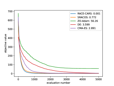
Region shrinking rate is configured to be $\gamma=0.9$ and $0.95$, with shrinking frequency of $\rho=0.01$ and $0.001$ for $n=50,500$, respectively. Each algorithm is executed over 30 trials, and the mean convergence trajectories of the best-so-far values are depicted in Figure 1 and Figure 2. The numerical values adjacent to the algorithm names in the legends represent the mean of the attained minima. It is evident that that RACE-CARS performs the best on both convergence speed and optimal value, with a slight edge to CMA-ES on the strongly convex Sphere function. Yet this comes at the cost of scalability due to CMA-ES’s reliance on an $n$-dimensional covariance matrix, which is significantly more computationally intensive compared to the other algorithms.

Prompt tuning for extremely large pre-trained language models (PTMs) has shown great power. PTMs such as GPT-3 (Brown et al. 2020) are usually released as a service due to commercial considerations and the potential risk of misuse, allowing users to design individual prompts to query the PTMs through black-box APIs. This scenario is called Language-Model-as-a-Service (LMaaS) (Diao et al. 2022; Sun et al. 2022). In this part we follow the experiments designed by (Sun et al. 2022) ¹¹1Code can be found in https://github.com/txsun1997/Black-Box-Tuning, where language understanding task is formulated as a classification task predicting for a batch of PTM-modified input texts $X$ the labels $Y$ in the PTM vocabulary, namely we need to tune the prompt such that the black-box PTM inference API $f$ takes a continuous prompt ${\mathbf{p}}$ satisfying $Y=f({\mathbf{p}};X).$ Moreover, to handle the high-dimensional prompt ${\mathbf{p}},$ (Sun et al. 2022) proposed to randomly embed the $D$-dimensional prompt ${\mathbf{p}}$ into a lower dimensional space $\mathbb{R}^{d}$ via random projection matrix ${\mathbf{A}}\in\mathbb{R}^{D\times d}.$ Therefore, the objective becomes:

where $\mathcal{Z}=[-50,50]^{d}$ is the search space and $\mathcal{L}(\cdot)$ is cross entropy loss.

In our experimental setup, we configure the search space dimension to $d=500$ and the prompt length to $50$, with RoBERTa (Liu et al. 2019a) serving as the backbone model. We evaluate performance on datasets SST-2 (Socher et al. 2013), Yelp polarity and AG’s News (Zhang, Zhao, and LeCun 2015), and RTE (Wang et al. 2018a). With a fixed API call budget of $T=8000,$ we pit RACE-CARS against SRACOS and the default DFO algorithm CMA-ES utilized in (Sun et al. 2022) ²²2 Our choice to exclude ZO-Adam and DE is based on their suboptimal performance with high-dimensional nonconvex black-box functions, as demonstrated in the last section..

For our tests, the shrinking rate is $\gamma=0.7$, with shrinking frequency of $\rho=0.002.$ Each algorithm is repeated 5 times independently with unique seeds. We assess the algorithms based on the mean and deviation of training loss, training accuracy, development loss and development accuracy. The SST-2 dataset results are highlighted in Figure 3, with additional findings for Yelp Polarity, AG’s News, and RTE detailed in the appendix. The results indicate that RACE-CARS consistently accelerates the convergence of SRACOS. While CMA-ES shows superior performance on Yelp Polarity, AG’s News, and RTE, it also exhibits signs of overfitting. RACE-CARS achieves comparable performance to CMA-ES, despite the latter’s hyperparameters being finely tuned. Notably, the hyperparameters for RACE-CARS were empirically adjusted based on the SST-2 dataset and then applied to the other three datasets without further tuning.

• (i)

  For discontinuous objective functions.

  Dimensionally local Holder continuity in Definition 5, imposes certain constraints on the objective through a set of continuous envelopes, whereas the objective is not supposed to be continuous. Beyond the continuous cases discussed in the previous section, RACE-CARS remains applicable to discontinuous objectives as well. Refer to appendix for a comprehensive understanding.

• (ii)

  For discrete optimization.

  Similar to SRACOS algorithm, RACE-CARS retains the capability to tackle discrete optimization problems. The convergence theorems, presented in Theorem 2 and Theorem 3, encompass this situation by altering the measure of probability space to be for example, induced by counting measure. We extend experiments on mixed-integer programming problems, substantiating the acceleration of RACE-CARS empirically. See appendix for details.

The concept hypothesis-target shattering, central to our discussion, draws inspiration from the established learning theory notion of shatter and its deep ties to the Vapnik-Chervonenkis (VC) theory (Vapnik et al. 1998). At the heart of VC theory lies the VC dimension, a measure of a hypothesis family’s capacity to distinguish among data points based on their labels. Specifically, for a collection of data points with binary labels, $S$, we say a subset $S^{\prime}\subseteq S$ is shattered by a hypothesis family $\mathcal{H}$ if there exists a hypothesis $h\in\mathcal{H}$ that perfectly aligns with the labels of points in $S^{\prime}$ and contrasts with those outside:

The shattering coefficient, $\mathcal{S}(\mathcal{H},n)$, signifies the variety of point-label combinations that $\mathcal{H}$ can produce for $n$ points. The VC dimension is then defined as $VC(\mathcal{H}):=\{\sup{n:\mathcal{S}(\mathcal{H},n)=2^{n}}\}$, indicating the maximum number of points that can be distinctly labeled by $\mathcal{H}$.

In the context of classification-based DFO, we represent the target-representative capability of a family of hypotheses through hypothesis-target shattering, measuring the overlap of hypothesis’s active region and the target. Therefore the quintessence of algorithm design hinges on maximizing this quantity. discerning the target-representative capacity within the intricate landscape of nonconvex, black-box optimization problems is nontrivial. Nonetheless, the target-representative capability of hypotheses family generated by RACOS, although proved under the previous framework, empirically suggests sufficient efficacy in scenarios where the objective function exhibits locally Holder continuouity. Looking ahead, altering the $Training$ and $Replacing$ sub-procedures inherited from SRACOS, which may ideally lead to a bigger shattering rate and maintain the easy-to-sample characterization, will be another extension direction of the current study.

While it’s an appealing goal to develop a universally effective DFO algorithm for black-box functions without the need for hyperparameter tuning, this remains an unrealistic aspiration. Our proposed algorithm, RACE-CARS, introduces two hyperparameters: shrinking-rate $\gamma$ and shrinking-frequency $\rho.$ For an $n$-dimensional optimization problem, we call $\gamma^{n\rho}$ shrinking factor of RACE-CARS. We take Ackley for a case study, design ablation experiments on the two hyperparameters of RACE-CARS to reveal the mechanism. We stipulate that we do not aim to identify a optimal combination of hyperparameters for maximizing the overlap with the target hypothesis. Instead, our aim is to provide empirical guidance for tuning these hyperparameters effectively. For further details, the reader is directed to the appendix.

References

- Akay and Karaboga (2012) Akay, B.; and Karaboga, D. 2012. Artificial bee colony algorithm for large-scale problems and engineering design optimization. Journal of intelligent manufacturing, 23: 1001–1014.
- Akiba et al. (2019) Akiba, T.; Sano, S.; Yanase, T.; Ohta, T.; and Koyama, M. 2019. Optuna: A next-generation hyperparameter optimization framework. In Proceedings of the 25th ACM SIGKDD international conference on knowledge discovery & data mining, 2623–2631.
- Bäck and Schwefel (1993) Bäck, T.; and Schwefel, H.-P. 1993. An overview of evolutionary algorithms for parameter optimization. Evolutionary computation, 1(1): 1–23.
- Bickel and Levina (2004) Bickel, P. J.; and Levina, E. 2004. Some theory for Fisher’s linear discriminant function,naive Bayes’, and some alternatives when there are many more variables than observations. Bernoulli, 10(6): 989–1010.
- Bogunovic et al. (2016) Bogunovic, I.; Scarlett, J.; Krause, A.; and Cevher, V. 2016. Truncated variance reduction: A unified approach to bayesian optimization and level-set estimation. Advances in neural information processing systems, 29.
- Brown et al. (2020) Brown, T.; Mann, B.; Ryder, N.; Subbiah, M.; Kaplan, J. D.; Dhariwal, P.; Neelakantan, A.; Shyam, P.; Sastry, G.; Askell, A.; et al. 2020. Language models are few-shot learners. Advances in neural information processing systems, 33: 1877–1901.
- Céa (1971) Céa, J. 1971. Optimisation: théorie et algorithmes. Jean Céa. Dunod.
- Chen et al. (2019) Chen, X.; Liu, S.; Xu, K.; Li, X.; Lin, X.; Hong, M.; and Cox, D. 2019. Zo-adamm: Zeroth-order adaptive momentum method for black-box optimization. Advances in neural information processing systems, 32.
- Conn, Scheinberg, and Vicente (2009) Conn, A. R.; Scheinberg, K.; and Vicente, L. N. 2009. Introduction to derivative-free optimization. SIAM.
- Diao et al. (2022) Diao, S.; Huang, Z.; Xu, R.; Li, X.; Lin, Y.; Zhou, X.; and Zhang, T. 2022. Black-box prompt learning for pre-trained language models. arXiv preprint arXiv:2201.08531.
- El-Yaniv and Wiener (2012) El-Yaniv, R.; and Wiener, Y. 2012. Active Learning via Perfect Selective Classification. Journal of Machine Learning Research, 13(2).
- Eriksson et al. (2019) Eriksson, D.; Pearce, M.; Gardner, J.; Turner, R. D.; and Poloczek, M. 2019. Scalable global optimization via local Bayesian optimization. Advances in neural information processing systems, 32.
- Falkner, Klein, and Hutter (2018) Falkner, S.; Klein, A.; and Hutter, F. 2018. BOHB: Robust and efficient hyperparameter optimization at scale. In International conference on machine learning, 1437–1446. PMLR.
- Fan and Fan (2008) Fan, J.; and Fan, Y. 2008. High dimensional classification using features annealed independence rules. Annals of statistics, 36(6): 2605.
- Fortin et al. (2012) Fortin, F.-A.; De Rainville, F.-M.; Gardner, M.-A. G.; Parizeau, M.; and Gagné, C. 2012. DEAP: Evolutionary algorithms made easy. The Journal of Machine Learning Research, 13(1): 2171–2175.
- Frazier (2018) Frazier, P. I. 2018. A tutorial on Bayesian optimization. arXiv preprint arXiv:1807.02811.
- Ge et al. (2022) Ge, D.; Liu, T.; Liu, J.; Tan, J.; and Ye, Y. 2022. SOLNP+: A Derivative-Free Solver for Constrained Nonlinear Optimization. arXiv preprint arXiv:2210.07160.
- Gotovos (2013) Gotovos, A. 2013. Active learning for level set estimation. Master’s thesis, Eidgenössische Technische Hochschule Zürich, Department of Computer Science,.
- Hall, Marron, and Neeman (2005) Hall, P.; Marron, J. S.; and Neeman, A. 2005. Geometric representation of high dimension, low sample size data. Journal of the Royal Statistical Society Series B: Statistical Methodology, 67(3): 427–444.
- Hansen (2016) Hansen, N. 2016. The CMA evolution strategy: A tutorial. arXiv preprint arXiv:1604.00772.
- Hashimoto, Yadlowsky, and Duchi (2018) Hashimoto, T.; Yadlowsky, S.; and Duchi, J. 2018. Derivative free optimization via repeated classification. In International Conference on Artificial Intelligence and Statistics, 2027–2036. PMLR.
- Hensman, Fusi, and Lawrence (2013) Hensman, J.; Fusi, N.; and Lawrence, N. D. 2013. Gaussian processes for big data. arXiv preprint arXiv:1309.6835.
- Hu, Qian, and Yu (2017) Hu, Y.-Q.; Qian, H.; and Yu, Y. 2017. Sequential classification-based optimization for direct policy search. In Proceedings of the AAAI Conference on Artificial Intelligence, volume 31.
- Larson, Menickelly, and Wild (2019) Larson, J.; Menickelly, M.; and Wild, S. M. 2019. Derivative-free optimization methods. Acta Numerica, 28: 287–404.
- Liao (2010) Liao, T. W. 2010. Two hybrid differential evolution algorithms for engineering design optimization. Applied Soft Computing, 10(4): 1188–1199.
- Liu et al. (2019a) Liu, Y.; Ott, M.; Goyal, N.; Du, J.; Joshi, M.; Chen, D.; Levy, O.; Lewis, M.; Zettlemoyer, L.; and Stoyanov, V. 2019a. Roberta: A robustly optimized bert pretraining approach. arXiv preprint arXiv:1907.11692.
- Liu et al. (2017) Liu, Y.-R.; Hu, Y.-Q.; Qian, H.; Qian, C.; and Yu, Y. 2017. Zoopt: Toolbox for derivative-free optimization. arXiv preprint arXiv:1801.00329.
- Liu et al. (2019b) Liu, Y.-R.; Hu, Y.-Q.; Qian, H.; and Yu, Y. 2019b. Asynchronous classification-based optimization. In Proceedings of the First International Conference on Distributed Artificial Intelligence, 1–8.
- Michalski (2000) Michalski, R. S. 2000. Learnable evolution model: Evolutionary processes guided by machine learning. Machine learning, 38: 9–40.
- Nayebi, Munteanu, and Poloczek (2019) Nayebi, A.; Munteanu, A.; and Poloczek, M. 2019. A framework for Bayesian optimization in embedded subspaces. In International Conference on Machine Learning, 4752–4761. PMLR.
- Nelder and Mead (1965) Nelder, J. A.; and Mead, R. 1965. A simplex method for function minimization. The computer journal, 7(4): 308–313.
- Nesterov and Spokoiny (2017) Nesterov, Y.; and Spokoiny, V. 2017. Random gradient-free minimization of convex functions. Foundations of Computational Mathematics, 17: 527–566.
- Opara and Arabas (2019) Opara, K. R.; and Arabas, J. 2019. Differential Evolution: A survey of theoretical analyses. Swarm and evolutionary computation, 44: 546–558.
- Ragonneau and Zhang (2023) Ragonneau, T. M.; and Zhang, Z. 2023. PDFO–A Cross-Platform Package for Powell’s Derivative-Free Optimization Solver. arXiv preprint arXiv:2302.13246.
- Ray and Saini (2001) Ray, T.; and Saini, P. 2001. Engineering design optimization using a swarm with an intelligent information sharing among individuals. Engineering Optimization, 33(6): 735–748.
- Ros and Hansen (2008) Ros, R.; and Hansen, N. 2008. A simple modification in CMA-ES achieving linear time and space complexity. In International conference on parallel problem solving from nature, 296–305. Springer.
- Scheinberg (2022) Scheinberg, K. 2022. Finite Difference Gradient Approximation: To Randomize or Not? INFORMS Journal on Computing, 34(5): 2384–2388.
- Shahriari et al. (2015) Shahriari, B.; Swersky, K.; Wang, Z.; Adams, R. P.; and De Freitas, N. 2015. Taking the human out of the loop: A review of Bayesian optimization. Proceedings of the IEEE, 104(1): 148–175.
- Shi et al. (2021) Shi, H.-J. M.; Xuan, M. Q.; Oztoprak, F.; and Nocedal, J. 2021. On the numerical performance of derivative-free optimization methods based on finite-difference approximations. arXiv preprint arXiv:2102.09762.
- Snoek, Larochelle, and Adams (2012) Snoek, J.; Larochelle, H.; and Adams, R. P. 2012. Practical bayesian optimization of machine learning algorithms. Advances in neural information processing systems, 25.
- Sobol’ (1967) Sobol’, I. M. 1967. On the distribution of points in a cube and the approximate evaluation of integrals. Zhurnal Vychislitel’noi Matematiki i Matematicheskoi Fiziki, 7(4): 784–802.
- Socher et al. (2013) Socher, R.; Perelygin, A.; Wu, J.; Chuang, J.; Manning, C. D.; Ng, A. Y.; and Potts, C. 2013. Recursive deep models for semantic compositionality over a sentiment treebank. In Proceedings of the 2013 conference on empirical methods in natural language processing, 1631–1642.
- Sun et al. (2022) Sun, T.; Shao, Y.; Qian, H.; Huang, X.; and Qiu, X. 2022. Black-box tuning for language-model-as-a-service. In International Conference on Machine Learning, 20841–20855. PMLR.
- Vapnik et al. (1998) Vapnik, V.; et al. 1998. Statistical learning theory.
- Wang et al. (2018a) Wang, A.; Singh, A.; Michael, J.; Hill, F.; Levy, O.; and Bowman, S. R. 2018a. GLUE: A multi-task benchmark and analysis platform for natural language understanding. arXiv preprint arXiv:1804.07461.
- Wang, Fonseca, and Tian (2020) Wang, L.; Fonseca, R.; and Tian, Y. 2020. Learning search space partition for black-box optimization using monte carlo tree search. Advances in Neural Information Processing Systems, 33: 19511–19522.
- Wang et al. (2018b) Wang, Z.; Gehring, C.; Kohli, P.; and Jegelka, S. 2018b. Batched large-scale Bayesian optimization in high-dimensional spaces. In International Conference on Artificial Intelligence and Statistics, 745–754. PMLR.
- Wang et al. (2016) Wang, Z.; Hutter, F.; Zoghi, M.; Matheson, D.; and De Feitas, N. 2016. Bayesian optimization in a billion dimensions via random embeddings. Journal of Artificial Intelligence Research, 55: 361–387.
- Yang and Shami (2020) Yang, L.; and Shami, A. 2020. On hyperparameter optimization of machine learning algorithms: Theory and practice. Neurocomputing, 415: 295–316.
- Yi et al. (2024) Yi, Z.; Wei, Y.; Cheng, C. X.; He, K.; and Sui, Y. 2024. Improving sample efficiency of high dimensional Bayesian optimization with MCMC. arXiv preprint arXiv:2401.02650.
- Yu (1979) Yu, W.-C. 1979. Positive basis and a class of direct search techniques. Scientia Sinica, Special Issue of Mathematics, 1(26): 53–68.
- Yu and Qian (2014) Yu, Y.; and Qian, H. 2014. The sampling-and-learning framework: A statistical view of evolutionary algorithms. In 2014 IEEE Congress on Evolutionary Computation (CEC), 149–158. IEEE.
- Yu, Qian, and Hu (2016) Yu, Y.; Qian, H.; and Hu, Y.-Q. 2016. Derivative-free optimization via classification. In Proceedings of the AAAI Conference on Artificial Intelligence, volume 30.
- Yue et al. (2023) Yue, P.; Yang, L.; Fang, C.; and Lin, Z. 2023. Zeroth-order Optimization with Weak Dimension Dependency. In The Thirty Sixth Annual Conference on Learning Theory, 4429–4472. PMLR.
- Zhang, Zhao, and LeCun (2015) Zhang, X.; Zhao, J.; and LeCun, Y. 2015. Character-level convolutional networks for text classification. Advances in neural information processing systems, 28.
Appendix A Appendix
Synthetic functions
-
•
Ackley:
Levy:
where
Rastrigin:
Sphere:
Beyond continuity