Saturation mechanism of the fluctuation dynamo in supersonic turbulent plasmas
Abstract
Magnetic fields in several astrophysical objects are amplified and maintained by a dynamo mechanism, which is the conversion of the turbulent kinetic energy to magnetic energy. A dynamo that amplifies magnetic fields at scales less than the driving scale of turbulence is known as the fluctuation dynamo. We aim to study the properties of the fluctuation dynamo in supersonic turbulent plasmas, which is of relevance to the interstellar medium of star-forming galaxies, structure formation in the Universe, and laboratory experiments of laser-plasma turbulence. Using numerical simulations of driven turbulence, we explore the global and local properties of the exponentially growing and saturated (statistically steady) state of the fluctuation dynamo for subsonic and supersonic turbulent flows. First, we confirm that the fluctuation dynamo efficiency decreases with compressibility. Then, we show that the fluctuation dynamo generated magnetic fields are spatially intermittent and the intermittency is higher for supersonic turbulence, but in both cases, the level of intermittency decreases as the field saturates. We also find a stronger back reaction of the magnetic field on the velocity for the subsonic case as compared to the supersonic case. Locally, we find that the level of alignment between vorticity and velocity, velocity and magnetic field, and current density and magnetic field in the saturated stage is enhanced in comparison to the exponentially growing phase for the subsonic case, but only the current density and magnetic field alignment is enhanced for the supersonic case. Finally, we show that both the magnetic field amplification (mainly due to weaker stretching of magnetic field lines) and diffusion decreases when the field saturates, but the diffusion is enhanced relative to amplification. This occurs throughout the volume in the subsonic turbulence, but primarily in the strong-field regions for the supersonic case. This leads to the saturation of the fluctuation dynamo. Overall, both the amplification and diffusion of magnetic fields are affected by the exponentially growing magnetic fields and thus a drastic change in either of them is not required for the saturation of the fluctuation dynamo.
pacs:
I Introduction
It is important to study the properties of magnetic fields in supersonic turbulent plasmas because of their applications to astrophysics [1, 2] and recently possible laboratory experiments of laser-plasma turbulence [3]. In the Sun, turbulent plasma in the convection zone is slightly supersonic [4, 5] and affects surface dynamics [6]. On galactic scales, turbulence in the interstellar medium (ISM) of star-forming galaxies is driven supersonically at a range of scales by a variety of mechanisms such as supernova explosions, gravitational collapse, accretion, and jets from young stellar objects and active galactic nuclei [7, 8, 9]. Magnetic fields in the supersonic turbulent plasma of the ISM play a crucial role in the present-day [10] and primordial [11, 12, 13, 14] star formation. The turbulence driven by structure formation in galaxy clusters can also be supersonic [15] and this affects cluster magnetic field structure, which in turn controls the acceleration and propagation of relativistic particles [16].
Physically, the strength and structure of observed magnetic fields in astrophysical objects [17, 6, 18] and derived magnetic fields in plasma turbulence experiments with a dynamically insignificant initial magnetic field [19, 20] can be largely explained by a turbulent dynamo, the mechanism by which the turbulent kinetic energy is converted to magnetic energy [1, 21]. Turbulence is prevalent in most astrophysical systems as the Reynolds number, (where is the driving scale of turbulence, is the root mean square (rms) velocity, and is the viscosity), is usually very high. A dynamo that amplifies magnetic fields at scales less than the driving scale of turbulence is known as the fluctuation or small-scale dynamo. In a turbulent (or even random) flow, the fluctuation dynamo exponentially amplifies (kinematic stage) a weak seed field of any form [22, 23] to dynamically significant strengths when the magnetic Reynolds number, ( is the resistivity, which controls magnetic diffusion), is greater than a critical value [ as shown in 24, 25, 26, 27, 28]. The critical value of the magnetic Reynolds number also depends on the [27, 29] and in this paper we explore the regime, which is applicable to both the subsonic, hot, and the supersonic, cold phases of the ISM [see Table 2 in 30]. This magnetic field amplification is primarily due to the stretching of magnetic field lines by turbulent motions [31, 32, 33]. Once the field becomes strong enough, it back reacts on the turbulent flow via the Lorentz force and then the dynamo saturates (saturated stage). The saturation mechanism, primarily studied for subsonic turbulence, is due to a combination of reduced amplification and diffusion [34, 35]. In this paper, using driven turbulence periodic box magnetohydrodynamic (MHD) simulations, we aim to study the saturation mechanism of the fluctuation dynamo in supersonic turbulent plasmas.
The fluctuation dynamo in subsonic turbulent plasma has been studied analytically [22, 24, 36, 37, 38, 39, 40, 34, 41], numerically [25, 42, 26, 43, 44, 45, 46, 35, 47], and recently via experiments [19, 20]. These studies confirm exponential growth of magnetic fields and show the following magnetic field properties: the saturated magnetic energy is a fraction of the turbulent kinetic energy, the magnetic power spectra in the kinematic stage seems to follow a power law with an exponent , and the magnetic field in the saturated stage has a higher correlation length than in the kinematic stage. Although not as extensively as for subsonic turbulence, the fluctuation dynamo in supersonic turbulent plasma is also studied analytically [48, 49, 50] and numerically [51, 52, 28, 23]. These studies show that with increasing compressibility, the critical magnetic Reynolds number increases and the fraction of turbulent kinetic energy getting converted to magnetic energy, per unit time, decreases. Thus, the overall efficiency of the dynamo decreases in supersonic turbulent plasmas as compared to their subsonic counterparts. However, the effect of compressibility on the local interaction of the magnetic and velocity fields and the saturation mechanism is not known yet. We aim to explore such questions with this study. Furthermore, some of the properties of the fluctuation dynamo are also seen in recent large-scale cosmological simulations of galaxies [53, 54, 55] and galaxy clusters [56, 57, 58]. The turbulence in these cosmological simulations would also be supersonic in regions with shocks and understanding the physics of the fluctuation dynamo in supersonic turbulent plasmas would further help understand magnetic fields during cosmological evolution.
The remainder of this paper is organised as follows. In Sec. II, we describe our numerical methods and parameters of the study. The results are presented and discussed in Sec. III and Sec. IV. In Sec. III, we describe the difference in the global (spectral and structural) properties of magnetic fields in the kinematic and saturated stages as a function of the compressibility of the turbulent flow. In Sec. IV, we study the local interaction of the velocity and magnetic fields in the kinematic and saturated stages for subsonic and supersonic flows. Finally, we summarise and conclude our results in Sec. V.
II Methods
To study the physics of the fluctuation dynamo in supersonic turbulent plasmas, we use a modified version of the FLASH code (version 4) [59, 60] to numerically solve the equations of compressible MHD (Eq. 1 - Eq. 4) for an isothermal gas (an isothermal equation of state is adopted for simplicity) in a triply periodic cartesian () domain of size with a uniform grid and grid points. We use the HLL3R (3-wave approximate) Riemann solver [61] to solve the following equations:
| (1) | |||
| (2) | |||
| (3) | |||
| (4) |
where is the density, is the velocity field, is the magnetic field, is the constant sound speed, is the traceless rate of strain tensor, is the prescribed acceleration field constructed using the Ornstein-Uhlenbeck process for the turbulent driving, and and are constant viscosity and resistivity, respectively.
The turbulent flow is driven solenoidally (, where is the wavenumber and is the forcing vector in space) on large scales () using a parabolic function of power with a peak at and zero power at [62, 23]. Thus, the effective driving scale of turbulence is approximately equal to . The correlation time of the forcing is set to the eddy turnover time of the turbulent flow, . We use purely solenoidal driving instead of compressive driving because solenoidal driving gives a higher dynamo efficiency [52, 47]. The diffusion of velocity and magnetic fields is characterised by the hydrodynamic (, where is the rms of the turbulent velocity) and magnetic () Reynolds numbers. The compressibility of the medium is quantified using the turbulent Mach number, .
We initialize our simulations with zero velocity, a uniform density (), and a very weak random seed field (plasma beta , where is the rms magnetic field strength). We select for all our runs and vary Rm in the range . Thus, the magnetic Prandtl number, Pm, is always greater than or equal to one and varies in the range . The main parameter of the study is the Mach number, which is varied from (subsonic) to (supersonic). We run all simulations till the dynamo saturates and the magnetic fields achieve a statistically steady state. For our set of selected parameters, the magnetic field saturates in less than ( is the eddy turnover time). We then study the properties of the velocity and magnetic fields in the kinematic and saturated stages for the subsonic and supersonic turbulent flows.
III Global fluctuation dynamo properties
Here, we first compare the properties of the time evolution of magnetic fields, i.e., the growth rate in the kinematic phase and the ratio of magnetic to turbulent kinetic energy in the saturated stage with existing studies. Then, we discuss the spectral and structural properties of velocity and magnetic fields in the kinematic and saturated stages for turbulent flows with low (, subsonic) and high (, supersonic) Mach numbers.

III.1 Growth rate, saturated level, structure, and spectra
Fig. 1 shows the evolution of the ratio of magnetic to turbulent kinetic energies, , as a function of time normalised by the eddy turnover time, , for various Mach numbers ( and ) with and . After the initial transient phase, the magnetic energy amplifies exponentially (kinematic stage) for all the cases. Then when the magnetic field becomes strong enough to react back on the flow, the exponential increase slows down, and finally the magnetic energy saturates to a statistically steady value (saturated stage). This happens for all the runs and the corresponding growth rate, , in the exponentially growing or kinematic stage and the saturated level of , , in the saturated stage are given in Table 1.
| Simulation Name | Rm | (kin) | (sat) | |||
|---|---|---|---|---|---|---|
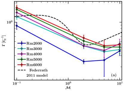

Fig. 2 shows the growth rate, , (Fig. 2 (a)) and the saturated level of , , (Fig. 2 (b)) as a function of . The growth rate decreases till but then increases for and the overall trend is consistent with the empirical model in the literature [52]. Fig. 2 (b) shows the dependence of the saturated level, , on . For all values of Rm, decreases with . This shows that as the compressibility increases, a smaller fraction of turbulent kinetic energy is converted to magnetic energy, per unit time. Thus, the efficiency of the fluctuation dynamo decreases with increasing compressibility. Here too, the trend of with roughly agrees with the known empirical model [52]. These empirical models for the dependence of and on are constructed from numerical simulations in [52], where most of the simulations used numerical viscosity and resistivity, whereas here, all our simulations include explicit (viscous and resistive) diffusion terms (Eq. 2 and Eq. 3). This might be the reason for differences in the results (coloured lines vs. dashed black line in Fig. 2), but the overall trend is roughly consistent with the empirical models. Thus, generally, the growth rates and the saturated levels agree with previous results. We now show and discuss velocity and magnetic structures in the kinematic and saturated stages for and with a fixed Rm of .


Fig. 3 and Fig. 4 shows two-dimensional velocity and magnetic field structures in the kinematic and saturated stages for subsonic and supersonic turbulence. Both the velocity and magnetic fields show random distributions with complex structures and without any significant mean trend. This is expected for the turbulent flows and the magnetic fields they amplify. The velocity structures for subsonic flow look larger in size in the saturated stage (Fig. 3 (b)) as compared to the kinematic stage (Fig. 3 (a)). This is due to the back reaction of the strong magnetic field on the turbulent flow (the back reaction is negligible in the kinematic stage). Such a difference is smaller for the supersonic case. The structures in supersonic turbulence (Fig. 3 (b, d)), in both the kinematic and saturated stages, are of a larger size than in the subsonic case (Fig. 3 (a, c)) but the supersonic case can have locally strong velocity because of random shocks. The difference in structure between the kinematic and saturated stages is more pronounced for the magnetic field. For both the Mach numbers, magnetic fields in the saturated stages (Fig. 4 (c, d)) have larger structures than in their corresponding kinematic stages (Fig. 4 (a, b)). Fig. 5 shows the three-dimensional magnetic structures in both the kinematic and saturated stages for both Mach numbers. Overall, for both Mach numbers, the magnetic fields have visually larger structures in the saturated stage than in their respective kinematic stage. We now discuss the spectral properties of velocity and magnetic fields in the kinematic and saturated stages for subsonic and supersonic turbulent flows.


The top panels of Fig. 6 show the shell-integrated turbulent kinetic (, Fig. 6 (a)) and magnetic energy (, Fig. 6 (b)) spectra, which were averaged over a few eddy turnover times ( for the kinematic stage and for the saturated stage) for the subsonic () and supersonic () cases. The turbulent kinetic energy spectra, over a range of wavenumbers (), are seen to be consistent with the Kolmogorov spectrum [63] for the subsonic turbulence and Burgers spectrum [64] for the supersonic turbulence (agreement is slightly better for the supersonic case). At smaller scales, the turbulent kinetic energy is higher for the supersonic case as compared to the subsonic case due to strong shocks. For the subsonic case, as the magnetic field saturates, the turbulent kinetic energy spectrum steepens and it shows the effect of the back-reaction due to the Lorentz force on the turbulent flow. However, this effect on the turbulent kinetic energy spectra for the supersonic case is not that significant. The magnetic energy spectra vary between the kinematic and saturated stages for both subsonic and supersonic flows (Fig. 6 (b)). At lower wavenumbers, the magnetic spectra in the kinematic stage seem to follow spectra as expected from Kazantsev’s analytical work [22]. The agreement seems to be better for the subsonic flow than the supersonic case and this is because Kazantsev’s theory is derived assuming incompressible flows. However, from extensions to Kazantsev’s theory [40], the slope of the magnetic power spectrum for the supersonic case in the kinematic stage might still be [28]. For both cases, the spectra flatten as the magnetic field saturates. On smaller scales, the magnetic energy is higher for the supersonic case in comparison to the subsonic one. This is primarily due to strong shocks and higher turbulent kinetic energy at smaller scales for supersonic turbulence.
We use the turbulent kinetic () and magnetic () energy spectra to compute the correlation (approximately average) length of the velocity () and magnetic () fields as
| (5) |
The bottom panels of Fig. 6 show the velocity (, Fig. 6 (c)) and magnetic field (, Fig. 6 (d)) correlation scale as a function of the normalised time, . After the initial transient phase, fluctuates around immediately for the supersonic case, but is initially lower () for the subsonic case in its kinematic stage. For subsonic flows, as the magnetic field grows, increases and reaches a value of in the saturated stage. Thus, the back reaction of the growing magnetic field on the velocity field enhances its correlation length. This is seen only for the subsonic case (can also be concluded from the steepening of the turbulent kinetic energy spectra in Fig. 6 (a)). For the magnetic field, after the initial transient phase, the correlation length remains roughly constant in the kinematic phase ( and for the subsonic and supersonic case, respectively) and then increases as the magnetic fields become strong enough to react back on the turbulent flow. In the saturated stage, reaches a statistically steady value (, similar for both Mach numbers). Overall, the magnetic field correlation length increases due to the growing magnetic field for both the subsonic and supersonic cases (this also agrees with the larger size of magnetic structures seen in Fig. 4 and Fig. 5 for the saturated stage in comparison to the kinematic stage for both cases). We now quantify the non-Gaussianity of these magnetic structures.
III.2 Magnetic intermittency


The fluctuation dynamo generated magnetic fields are non-Gaussian or spatially intermittent and we aim to quantify the intermittency using the statistical measure kurtosis, , which for any random function with mean zero is defined as
| (6) |
where denote the average over the entire domain. The kurtosis of a Gaussian distribution is three.
First, in Fig. 7 (a), we show the probability distribution function (PDF) of a single component (here, ) of the random velocity field, , obtained in subsonic and supersonic turbulence in the kinematic and saturated stages of the fluctuation dynamo. The distribution, for all four cases, is very close to a Gaussian (or normal) distribution (the computed kurtosis is very close to that of a Gaussian, three). Thus, random velocity in these driven turbulence simulations always follows an approximately Gaussian distribution [also see 65].


Even though the turbulent velocity is normally distributed, the magnetic field it generates is non-Gaussian or spatially intermittent, as shown by Fig. 7 (b), which shows the PDF of a single component of the random magnetic field, , in their kinematic and saturated stages for subsonic and supersonic turbulent flows. The magnetic field is always more intermittent for the supersonic turbulence than the subsonic one. Moreover, for both cases, the magnetic intermittency decreases as the dynamo saturates. These conclusions can also be confirmed via the computed kurtosis values (Table 1 and Fig. 8). Fig. 8 (a) shows that the kurtosis, in the Rm range , does not depend much on Rm but increases with for both the kinematic and saturated stages. The difference in kurtosis of the magnetic fields between the kinematic and saturated stages increases with the Mach number of the turbulent flow, (Fig. 8 (b)). Thus, the non-Gaussian or intermittent nature of the dynamo generated magnetic fields is enhanced with compressibility.
Fig. 9 shows the PDF of for the subsonic and supersonic cases in their respective kinematic (Fig. 9 (a)) and saturated (Fig. 9 (b)) stages. We fit the PDF of with a normal distribution of form,
| (7) |
where (mean) and (standard deviation) are parameters of the fit. The black, dashed lines in Fig. 9 show the fitted distributions, and parameters of the fit are given in the legend. For the kinematic phase (Fig. 9 (a)), the lognormal distribution for is a better fit to the supersonic case as compared to the subsonic one. Also, the fit worsens for the saturated stage. Overall, the lognormal distribution captures high probability regions quite well in the kinematic phase and performs better for supersonic turbulence. The parameters and are also higher in the kinematic stage as compared to the saturated stage and are always higher for the supersonic flows. This further confirms that the degree of magnetic intermittency decreases as the field saturates and increases with the compressibility of the turbulent flow.
After characterising the global properties of velocity and magnetic fields in the fluctuation dynamo, in the next section, we study the local interaction of velocity and magnetic fields to explore the saturation mechanism of the fluctuation dynamo.
IV Local dynamics and the saturation mechanism
To understand the saturation mechanism of the fluctuation dynamo in subsonic and supersonic turbulent plasmas, here, we investigate the local properties and interactions of velocity and magnetic fields. This is also motivated by the fact that the fluctuation dynamo generated magnetic field is spatially intermittent (Sec. III.2) and thus we would expect that the back reaction of the magnetic field would be enhanced (locally and statistically) in strong-field regions (regions with magnetic field energy higher than the rms value, ).


First, we look at the properties of the following two dynamically important quantities, vorticity () and current density (), which are defined as the curl of the velocity () and magnetic field (),
| (8) |
Vorticity and current density characterise the local structure of the velocity and magnetic fields, respectively. The evolution of the rms (since the mean is zero) vorticity and current density is shown in Fig. 10. Once the turbulence is established, is statistically steady and is slightly higher in the subsonic case. The current density evolution is very similar to that of the magnetic fields, i.e., exponential growth and then saturation. The growth rate of is roughly half of the magnetic field growth rate for each case (Fig. 1 and Table 1) and is higher for the subsonic flows. The saturation level of the rms current density, , is higher for the supersonic case compared to the subsonic case (note that the initial value, , is the same for both subsonic and supersonic cases). Fig. 11 shows the pdfs of (Fig. 11 (a)) and (Fig. 11 (b)) for the kinematic and saturated stages of the dynamo with subsonic and supersonic turbulent flows. Both vorticity and current density distributions are non-Gaussian and the non-Gaussianity (quantified by kurtosis) for both cases is higher for the supersonic turbulence than the subsonic one. For the subsonic case, the kurtosis of decreases as the field saturates and thus vorticities significantly stronger than the rms value are suppressed in the saturated stage in comparison to the kinematic stage. This is a direct consequence of the back reaction of magnetic fields on the velocity field, i.e., the structure of the flow is locally altered. Such a statistically significant difference in the vorticity distribution is not seen for the supersonic turbulent flow. This also agrees with the conclusion from studying the evolution of velocity correlation length in Fig. 6 (c). On the other hand, the current density distribution for both the subsonic and supersonic flows is less intermittent in the saturated stage compared to their respective kinematic stages (compare the computed kurtosis given in the legend of Fig. 11(b)). Thus, the magnetic field in the saturated stage is structurally different than in the kinematic stage and for the supersonic turbulence in comparison to the subsonic case (global differences shown in Fig. 4, Fig. 5, Fig. 6, and Fig. 7). In the next subsection, we look at local interactions in terms of angles between the following vector quantities: vorticity, velocity, current density, and magnetic fields.
IV.1 Local interactions in terms of relevant angles


After confirming the change in the local structure of the velocity and magnetic field on saturation, here, we study the local interaction between those two vectors. First, the evolution of vorticity, obtained by taking the curl of the Navier-Stokes equation (the baroclinic term is zero for an isothermal equation of state), is [66, 67]
| (9) |
where the first term on the right-hand side represents growth of vorticity, the second term represents vorticity diffusion, the third term is due to density gradients, and the last term is due to the Lorentz force, ( is the speed of light). Since, we start with a zero velocity (and vorticity) and very weak magnetic fields, the vorticity is most likely generated by the third term when the density gradients develop and is then amplified by the first term [see Fig. 10 and in 67, 52]. The amplification of the vorticity field, via the first term, depends on the angle between and .
Another two angles of interest are the angle between the velocity and magnetic field, which controls the magnetic field induction term (first term in the right-hand side of Eq. 3) and the angle between the current density and magnetic field, which controls the Lorentz force (or the back reaction of the velocity field on the flow). Thus, we compute the cosine of the following three relevant angles,
| (10) | ||||
| (11) | ||||
| (12) | ||||
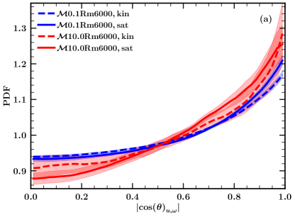
implies an angle of (or ) between the two vectors and thus maximum effect of the physically relevant term (for example, angle of between and implies maximum induction). On the other hand, implies alignment (or anti-alignment) between them and no effect of the term. Fig. 12 shows the total and conditional (for strong magnetic field regions, ) PDFs of these three angles in the kinematic and saturated stages for the subsonic and supersonic turbulence. We only show the absolute value of these angles as these distributions are symmetric around for isotropic random velocity and magnetic fields. For all three angles, as expected from isotropic random fields, all possible values of have a non-zero probability. However, all angles are not equiprobable and there are clear differences in the distributions with the Mach number of the turbulent flow and the dynamo stage. We discuss these differences and their implications below.
For the subsonic turbulence, the vorticity is slightly more aligned with the velocity in the saturated stage as compared to the kinematic stage (the difference is not much in Fig. 12 (a) but see Fig. 12 (b)). This shows that as the magnetic field grows, the vorticity amplification term is probably suppressed, especially in the strong-field regions. This is a direct consequence of the back reaction of the magnetic field on the flow. Such a difference is not statistically significant for the supersonic turbulence. This is consistent with our previous results (Fig. 6 (c) and Fig. 11 (a)) that the effect of the back reaction on the velocity in the supersonic case is negligible.
The angle between and controls the magnetic induction or amplification term and the alignment between and is statistically higher in the saturated stage as compared to the kinematic stage for subsonic turbulence (Fig. 12 (c)) and the difference is not that significant for the supersonic turbulence (even for the strong-field regions, Fig. 12 (d)). This mostly implies a reduction in induction due to enhanced alignment between and for the subsonic case but not so much for the supersonic case (because of locally strong shocks). Thus, for the subsonic turbulence, the magnetic field evolves in such a way as to enhance the level of alignment between the velocity and magnetic field.
Finally, the back reaction of the magnetic field on the velocity field via the Lorentz force is controlled by the angle between and , for which the alignment is enhanced in the saturated stage as compared to the kinematic stage (Fig. 12 (e)). However, here, the difference is higher for the supersonic case as compared to the subsonic one. The effect is enhanced in the strong-field regions, i.e., the field is more aligned with the current density where the magnetic energy is higher than its rms value (Fig. 12 (f)). In the saturated stage of the subsonic turbulence, the enhanced level of alignment between and would diminish the Lorentz force and the field advection by velocity would become dominant. This would give rise to a higher level of alignment between the velocity and magnetic field, which we see in Fig. 12 (c). Such a difference is not seen in the case of supersonic turbulence because of the presence of strong shocks.
IV.2 Characteristic magnetic scales

Besides the correlation length of the magnetic field (Fig. 6 (d)), the following characteristic magnetic length scales (or equivalently wavenumbers) can be used to further study the local magnetic field structure [36, 42],
| (13) | ||||
| (14) | ||||
| (15) | ||||
| (16) |
These wavenumbers (or length scales) can be related to the physical effects and structure of magnetic fields. is a probe of variation of the magnetic field along itself and is related to the length scale associated with greatest stretching of magnetic field lines (which maximises magnetic field amplification). is a probe of the magnetic field across itself and is related to resistive dissipation. is a probe of magnetic field variations along a direction perpendicular to both magnetic field () and Lorentz force () and is related to highest compressive motions (maximising the effect of compression on magnetic field). measures the overall variation of magnetic fields. For a subsonic fluctuation dynamo with , it is shown that the magnetic field organises itself into folded structures [42, 68]. Furthermore, the structures are folded sheets in the kinematic stage (identified by the condition, ) and folded ribbons in the saturated stage (identified by the condition, ). Since our simulations are with (highest Pm is , for and runs), we do not necessarily expect to see such folded structures. However, we compute these characteristic scales (Eq. 13 – Eq. 16) to further study the dynamics of growing and saturated magnetic fields in subsonic and supersonic turbulence.
Fig. 13 shows the temporal evolution of wavenumbers, (a), (b), (c), and (d), for subsonic () and supersonic () turbulent flows (both at ). Furthermore, the average values of these wavenumbers with one-sigma fluctuations in the kinematic and saturated stages are provided in the legend. For subsonic turbulence, in the kinematic stage, , and thus magnetic structures can probably be characterised as folded ribbons, but structures in the saturated stage are neither folded ribbons nor folded sheets. All four wavenumbers decrease as the magnetic field saturates for the subsonic case.
For the supersonic turbulence, based on these wavenumbers, the structures are never folded sheets or folded ribbons. All wavenumbers except decrease as the field grows and saturates. This shows that the dissipation takes place at a smaller length scale in the saturated stage as compared to the kinematic stage for the supersonic turbulence. However, the overall magnetic wavenumber, , still increases. The length scales associated with both the greatest stretching and compression also grows as the magnetic field saturates. On comparing all four wavenumbers between subsonic and supersonic turbulence, and are always smaller for the subsonic flow, but and are comparable in the kinematic stage and are higher for the supersonic case in the saturated stage. This shows that the length scale associated with greatest stretching and compression grow as the field saturates for both the subsonic and supersonic cases. However, as the magnetic field grows and saturates, the resistive dissipation scale increases for the subsonic case, but decreases for the supersonic case. The overall magnetic field scale grows as the magnetic field saturates for both Mach numbers (same as the magnetic correlation length in Fig. 6 (d)).
IV.3 Local stretching and compression of magnetic field lines, and magnetic field diffusion


We now study the local stretching and compression of magnetic field lines by the turbulent velocity using the eigenvalues and eigenvectors of the strain tensor. Such an analysis is done for isotropic subsonic turbulence [36, 35, 68], with a different motivation for slightly supersonic turbulence [ in 69], and for different setups such as magnetic fields in rotating convection simulations [70] and decaying magnetic field simulations [71]. Here, we aim to understand the effect of growing magnetic fields and compressibility on the local stretching and compression of magnetic field lines by analysing the strain tensor. First, we compute the strain tensor, , at each point in the domain using a sixth-order finite difference scheme and then calculate its eigenvalues () and eigenvectors (). We then arrange the eigenvalues in the order and let the corresponding eigenvectors be and . For an incompressible flow, the sum of eigenvalues, (approximately applicable for our subsonic case) and and [72, 73]. This need not be the case for our supersonic runs. In general, (positive ) corresponds to the direction of local magnetic field line stretching, (negative ) corresponds to the direction of local magnetic field line compression, and (also referred to as the ‘null’ direction) can be either, depending on the sign of [36, 42] (especially, see Fig. 10 in [42]). The magnitude of (when it is positive) and (when it is negative) can be considered as the strength of local magnetic field line stretching and compression, respectively. For clarity, throughout the rest of the paper, we refer and as , and and the corresponding eigenvectors as , and .
Fig. 14 show the PDF of all three eigenvalues normalised to the rms velocity for subsonic (, a) and supersonic (, b) turbulence in kinematic and saturated stages. As expected, for the subsonic case, it can be seen that is always negative and is always positive. This is not the case for the supersonic run, i.e., can be positive for (though the probability of this happening is low, see Fig. 14 (b)). When , the magnetic field is unaffected along the direction. The magnitude of is always smaller than the other two eigenvalues. On average, and this is consistent with previous results for isotropic hydrodynamic turbulence [73]. The absolute value of all three eigenvalues is smaller for the supersonic case (compare -axis in Fig. 14 (a) and Fig. 14 (b)). Thus the efficiency of local stretching and compression of magnetic field lines, which leads to magnetic field amplification, is lower for supersonic turbulence. This is also probably the reason for the smaller ratio of saturated magnetic to kinetic energy for compressible runs (see Fig. 2 (b)). As the magnetic field saturates, the absolute value of all three eigenvalues statistically decreases for the subsonic case, but increases for the supersonic case (as shown by the mean value in the legend of Fig. 14). Thus, the local field line stretching and compression decreases for the subsonic case in the saturated stage, but increases in the supersonic case. This is probably to counter high enhancement in diffusion compared to amplification for supersonic turbulence (see Fig. 12 and Table 2).


The amplification of magnetic fields due to field line stretching will be maximal when the field line stretching direction () is aligned with the magnetic field. Similarly, the effect of field line compression is maximal when the field line compression direction () is perpendicular to the local magnetic field. Fig. 15 show the total (Fig. 15 (a, c, e)) and conditional (based only on the strong-field regions, , Fig. 15 (b, d, f)) PDF of the angle between all three eigenvectors ( and ) and magnetic fields () in the kinematic and saturated stages for subsonic and supersonic turbulent flows. For the supersonic case (see Fig. 14 (b)), we only consider those regions where (implying local magnetic field line compression) and (implying local magnetic field line stretching). All the possible angles between these three eigenvectors and magnetic fields are not equiprobable.
In the kinematic stage, for the subsonic turbulence, the highest probable angle between the field line compression direction and magnetic field is and that between the field line stretching direction and magnetic field is . Thus, the magnetic field is more aligned with the field line stretching direction (and also the null direction) and perpendicular to the direction of the field line compression direction. This maximises magnetic field amplification. This also suggest that the magnetic field statistically lies more in the plane. As the field saturates in subsonic turbulence, the more probable angles for both and lie in the range of ( is still more aligned with , but the level of alignment has decreased). Thus, the amplification due to field line stretching and the effect of local compression is reduced in the saturated stage as compared to the kinematic stage via changes in these alignments. Moreover, these differences between the kinematic and saturated stages are enhanced in the strong-field regions (Fig. 15 (b, d, f)).
These trends are different for supersonic turbulence. In the kinematic stage, the magnetic field is overall more aligned with the and and also orthogonal to as in the subsonic case. Thus, here too, the magnetic field statistically lies in the plane. However, as the field saturates, the difference in the distribution of these angles is not as significant as in the subsonic case. In fact, is more aligned with in the saturated stage (although not in the strong-field regions; see Fig. 15 (b)), enhancing the effect of local compression regions with . On the other hand, in strong-field regions (Fig. 15 (f)), the orthogonality between and is slightly enhanced in the saturated stage, but the overall distribution of (Fig. 15 (e)) is roughly the same for both the kinematic and saturated stages.


We now explore the magnetic energy evolution equation and directly calculate the local growth and dissipation terms. The evolution of magnetic energy, for a fixed resistivity, , can be described by the following equation (see Sec. A for the derivation),
| (17) |
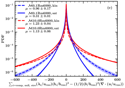
The first term is due to stretching and compression of magnetic field lines by the turbulent flow and can increase (e.g., by stretching of magnetic field lines) or decrease (e.g., unstretching of magnetic field lines) the magnetic energy. Statistically, both can happen in a turbulent medium. This term is computed as follows. First, the local magnetic field is projected along the three eigenvectors of the rate of strain tensor ( and ) and let these projected vectors be and . The first term is then calculated as the sum . The second term can also reduce or enhance magnetic energy locally depending on the divergence of the velocity. As expected, this term is negligible for the subsonic case, but does play an important role in the supersonic turbulence. The third term is the dissipative term, which always reduces the magnetic energy.
Fig. 16 shows the total and conditional (only in the strong-field regions) PDFs of the first, second, and first and second terms combined of Eq. 17 for subsonic and supersonic turbulence. For the subsonic case, the second term makes a small difference since is negligible. Thus, the magnetic field growth term (first term or combination of first two terms in the magnetic energy evolution equation for the subsonic case, Eq. 17) statistically decreases as the dynamo saturates. This implies that the growing magnetic field reduces its own amplification. The differences are further enhanced in strong-field regions (Fig. 16 (f)). For the supersonic case, the combined term is statistically higher in comparison to the subsonic one, but there is not much difference between the corresponding kinematic and saturated stages (Fig. 16 (e), also very similar mean value, , for the kinematic and saturated stages). In strong-field regions, the local growth term is slightly reduced on saturation for the supersonic case. Thus, on saturation, the local growth term is reduced throughout the volume for the subsonic case, but mostly in the strong-field regions for the supersonic case. However, the mean of the local growth term ( in Fig. 16 (e) and Fig. 16 (f)) always remains positive for all cases. Thus, the magnetic field always grows. Even in the saturated state, the magnetic energy is amplified to counter diffusion.
Fig. 17 show the PDF for the last term on the right-hand side of Eq. 17, , which probes the dissipation of magnetic energy. The dissipation is also statistically higher for the supersonic case in comparison to the subsonic one. For both cases, the magnetic dissipation statistically decreases as the dynamo saturates and the decrease is more statistically significant for the strong-field regions.
| Simulation Name | kin | sat | (kin - sat) | kin, | sat, | (kin - sat), |
|---|---|---|---|---|---|---|
Table 2 shows the ratio of the mean value of local growth term ( to the mean value of the local dissipation term () in the kinematic and saturated stages for subsonic and supersonic turbulence (the magnetic resistivity, , is the same for both runs). The ratio is always higher in the kinematic stage as compared to the saturated stage (see (kin-sat) in Table 2), especially in the strong-field regions. Note that, unlike the subsonic case, the difference of the ratio between the kinematic and saturated stages is small for the supersonic case and turns out to be significant only in the strong-field regions. Thus, although both growth and dissipation of magnetic fields decrease as the field saturates, the magnetic dissipation relative to the amplification is enhanced. This leads to the saturation of the fluctuation dynamo.
V Summary and Conclusions
Using driven turbulence numerical simulations, we explore the saturation mechanism of the fluctuation dynamo. Our main aim was to study the effect of compressibility on the dynamo generated fields and the saturation mechanism. We numerically solve the equations of non-ideal compressible MHD for an isothermal gas (Eq. 1 – Eq. 4) with very weak seed magnetic fields (random with mean zero) and primarily vary the Mach number, , of the turbulent driving. For all the cases, the magnetic field first amplifies exponentially (kinematic stage) and then saturates (saturated stage). We first study the global (over the entire domain) dynamo properties (growth rate, saturation level, spectra, and magnetic intermittency) as a function of . Then we explore the local properties and interactions of velocity and magnetic fields for subsonic () and supersonic () turbulent flows in the kinematic and saturated stages of the fluctuation dynamo. For the local study, we also isolate and study the regions with higher magnetic energy () as we expect that the dynamical effects of magnetic fields would be stronger in those regions. We summarize and conclude our key results below:
-
•
The growth rate of the magnetic energy decreases till and then increases for (Fig. 2 (a)). The fraction of turbulent kinetic energy getting converted to magnetic energy, per unit time, decreases with increasing (Fig. 2 (b)). Thus, the overall efficiency of the dynamo decreases as the compressibility increases.
-
•
The turbulent kinetic energy in the kinematic stage, over a range of wavenumbers, seems to follow the Kolmogorov power spectrum for subsonic turbulence and the Burgers power spectrum for supersonic turbulence (Fig. 6 (a)). As the field saturates, the kinetic energy power spectrum steepens for the subsonic case (also reflected in the velocity correlation length, Fig. 6 (c)) and such a change is not that significant in the supersonic stage. In the kinematic stage, the magnetic energy power spectrum is consistent, at larger scales, with the Kazantsev spectrum (the agreement is better for the subsonic turbulence). The magnetic spectra for both subsonic and supersonic flows are flatter at larger scales in the saturated stage (Fig. 6 (b)). The computed magnetic field correlation length also increases for both Mach numbers as the dynamo saturates (Fig. 6 (d)).
-
•
The velocity fields for both subsonic and supersonic turbulence roughly follows a Gaussian distribution (Fig. 7 (a)), the magnetic fields they amplify are non-Gaussian or spatially intermittent (Fig. 7 (b)). The intermittency decreases for both Mach numbers as the field saturates, but is always higher for the supersonic case (Fig. 8). Furthermore, in the kinematic stage, the PDF of roughly follows a lognormal distribution and the fit is better for the supersonic case. The effects of enhanced magnetic intermittency with compressibility must be considered while studying the effects of the fluctuation dynamo action in star-forming regions.
-
•
Locally, for the subsonic turbulence, we find that the level of alignment between the velocity and vorticity, velocity and magnetic fields, and magnetic fields and current density is enhanced as the magnetic field saturates (Fig. 12). However, for the supersonic case, the distribution of angles between the velocity and vorticity and vorticity and magnetic fields remains statistically the same in both stages and only the level of alignment between current density and magnetic fields is enhanced on saturation. This shows that back-reaction of the growing magnetic field on the velocity field is not that significant in supersonic turbulence in comparison to subsonic flows.
-
•
We also compute the evolution of following characteristic magnetic length scales: length scales associated with highest stretching of magnetic field lines (Eq. 13), resistive dissipation (Eq. 14), highest compression of magnetic field lines (Eq. 15), and overall field variation (Eq. 16). Based on these scale, magnetic field structures in the kinematic stage of the subsonic turbulence can probably be considered as folded ribbons, but magnetic structures in the saturated stage and in both stages for the supersonic case are neither folded sheets nor ribbons. As the field saturates, all of these length scales are enhanced for the subsonic case and all but the length scale associated with the resistive dissipation is enhanced for the supersonic case (Fig. 13).
-
•
We compute the eigenvalues and eigenvectors of the rate of strain tensor to study the local magnetic field line stretching and compression. The effect of the velocity is maximised when the direction of the magnetic field line stretching is aligned with the magnetic field and the direction of the magnetic field line compression is orthogonal to the magnetic field. In subsonic turbulence, the level of alignment and orthogonality of direction of stretching and compression with the magnetic field, respectively, is reduced as the field saturates. However, for the supersonic case, the difference between the kinematic and saturated stages in not that significant (Fig. 15). The magnetic field is slightly more orthogonal with the local compression direction in the saturated stage (although not in the strong-field regions), which enhances the effect of local compression.
-
•
Finally, we compute each term in the magnetic energy evolution equation (Eq. 17) and show that both the local growth (Fig. 16) and dissipation (Fig. 17) of magnetic fields decreases as the field saturates for the subsonic case. For the supersonic case, overall, there is not much difference in the local growth between the kinematic and saturated stages, but the local growth is reduced in the strong-field regions. As in the subsonic case, the dissipation is also reduced in the saturated stage for supersonic flows (Fig. 17). However, even though both the amplification and dissipation of magnetic fields statistically decreases as the field saturates, the dissipation relative to the amplification is enhanced (Table 2). Thus, the exponentially growing magnetic fields evolve to alter both the amplification and dissipation mechanisms of the fluctuation dynamo to achieve saturation. This also implies that a drastic change in either of them is not required. This change is significant throughout the volume for the subsonic case, but primarily occurs in strong-field regions for the supersonic turbulence.
Acknowledgements.
We thank both referees for their useful suggestions and comments. A. S. thanks Paul Bushby, Anvar Shukurov, and Toby Wood for useful discussions. C. F. acknowledges funding provided by the Australian Research Council (Discovery Project DP170100603 and Future Fellowship FT180100495), and the Australia-Germany Joint Research Cooperation Scheme (UA-DAAD). We further acknowledge high-performance computing resources provided by the Leibniz Rechenzentrum and the Gauss Centre for Supercomputing (grants pr32lo, pr48pi, and GCS Large-scale project 10391), and the Australian National Computational Infrastructure (grant ek9) in the framework of the National Computational Merit Allocation Scheme and the ANU Merit Allocation Scheme.Appendix A Evolution of magnetic energy in supersonic plasmas
Here, we derive the magnetic energy evolution equation from the induction equation,
| (18) |
For a constant , taking a dot product of Eq. 18 with and then integrating over the volume, V, gives
| (19) | |||
| (20) |
The right-hand side term in the above equation represents the evolution of magnetic energy.
Simplifying the first term further,
| (21) | |||
| (22) | |||
| (23) | |||
| (24) | |||
| (25) | |||
| is the rate of strain tensor, | |||
| (26) | |||
| (27) | |||
| (28) | |||
| (29) |
The last term in the above equation, being a surface integral, integrates out to zero for periodic boundary conditions.
Simplifying the second term further,
| (30) | |||
| (31) | |||
| (32) | |||
| (33) | |||
| (34) | |||
| (35) | |||
| (36) | |||
| (37) |
Thus, the magnetic energy evolution equation is
| (38) |
References
- Brandenburg and Subramanian [2005] A. Brandenburg and K. Subramanian, Astrophysical magnetic fields and nonlinear dynamo theory, Phys. Rep. 417, 1 (2005).
- Federrath [2016] C. Federrath, Magnetic field amplification in turbulent astrophysical plasmas, Journal of Plasma Physics 82, 535820601 (2016).
- Bott et al. [2020a] A. F. A. Bott, L. Chen, G. Boutoux, T. Caillaud, A. Duval, M. Koenig, B. Khiar, I. Lantuéjoul, L. Le-Deroff, B. Reville, R. Rosch, D. Ryu, C. Spindloe, B. Vauzour, B. Villette, A. A. Schekochihin, D. Q. Lamb, P. Tzeferacos, G. Gregori, and A. Casner, Inefficient magnetic-field amplification in supersonic laser-plasma turbulence, arXiv e-prints , arXiv:2008.06594 (2020a), arXiv:2008.06594 [physics.plasm-ph] .
- Cattaneo et al. [1990] F. Cattaneo, N. E. Hurlburt, and J. Toomre, Supersonic Convection, Astrophys. J. Lett. 349, L63 (1990).
- Weiss and Proctor [2014] N. O. Weiss and M. R. E. Proctor, Magnetoconvection, Cambridge Monographs on Mechanics (Cambridge University Press, 2014).
- Mart\́mathrm{i}nez Pillet [2013] V. Mart\́mathrm{i}nez Pillet, Solar Surface and Atmospheric Dynamics. The Photosphere, SSRv 178, 141 (2013), arXiv:1301.6933 [astro-ph.SR] .
- Mac Low and Klessen [2004] M.-M. Mac Low and R. S. Klessen, Control of star formation by supersonic turbulence, Reviews of Modern Physics 76, 125 (2004), arXiv:astro-ph/0301093 [astro-ph] .
- Elmegreen [2009] B. G. Elmegreen, Star Formation in Disks: Spiral Arms, Turbulence, and Triggering Mechanisms, in The Galaxy Disk in Cosmological Context, Vol. 254, edited by J. Andersen, Nordströara, B. m, and J. Bland-Hawthorn (2009) pp. 289–300, arXiv:0810.5406 [astro-ph] .
- Federrath et al. [2017] C. Federrath, J. M. Rathborne, S. N. Longmore, J. M. D. Kruijssen, J. Bally, Y. Contreras, R. M. Crocker, G. Garay, J. M. Jackson, L. Testi, and A. J. Walsh, The link between solenoidal turbulence and slow star formation in G0.253+0.016, in The Multi-Messenger Astrophysics of the Galactic Centre, IAU Symposium, Vol. 322, edited by R. M. Crocker, S. N. Longmore, and G. V. Bicknell (2017) pp. 123–128, arXiv:1609.08726 [astro-ph.SR] .
- Krumholz and Federrath [2019] M. R. Krumholz and C. Federrath, The Role of Magnetic Fields in Setting the Star Formation Rate and the Initial Mass Function, Frontiers in Astronomy and Space Sciences 6, 7 (2019), arXiv:1902.02557 [astro-ph.GA] .
- Sur et al. [2010] S. Sur, D. R. G. Schleicher, R. Banerjee, C. Federrath, and R. S. Klessen, The Generation of Strong Magnetic Fields During the Formation of the First Stars, Astrophys. J. Lett. 721, L134 (2010), arXiv:1008.3481 [astro-ph.CO] .
- Federrath et al. [2011a] C. Federrath, S. Sur, D. R. G. Schleicher, R. Banerjee, and R. S. Klessen, A New Jeans Resolution Criterion for (M)HD Simulations of Self-gravitating Gas: Application to Magnetic Field Amplification by Gravity-driven Turbulence, Astrophys. J. 731, 62 (2011a), arXiv:1102.0266 [astro-ph.SR] .
- Klessen [2019] R. Klessen, Formation of the first stars, in Formation of the First Black Holes, edited by M. Latif and D. Schleicher (2019) pp. 67–97.
- Sharda et al. [2021] P. Sharda, C. Federrath, M. R. Krumholz, and D. R. G. Schleicher, Magnetic field amplification in accretion discs around the first stars: implications for the primordial IMF, Mon. Not. R. Astron. Soc. 10.1093/mnras/stab531 (2021), arXiv:2007.02678 [astro-ph.GA] .
- Vazza et al. [2017] F. Vazza, T. W. Jones, M. Brüggen, G. Brunetti, C. Gheller, D. Porter, and D. Ryu, Turbulence and vorticity in Galaxy clusters generated by structure formation, Mon. Not. R. Astron. Soc. 464, 210 (2017), arXiv:1609.03558 [astro-ph.CO] .
- Brunetti and Jones [2014] G. Brunetti and T. W. Jones, Cosmic Rays in Galaxy Clusters and Their Nonthermal Emission, International Journal of Modern Physics D 23, 1430007-98 (2014), arXiv:1401.7519 [astro-ph.CO] .
- Govoni and Feretti [2004] F. Govoni and L. Feretti, Magnetic Fields in Clusters of Galaxies, International Journal of Modern Physics D 13, 1549 (2004).
- Beck [2016] R. Beck, Magnetic fields in spiral galaxies, Ann. Rev. Astron. Astrophys. 24, 4 (2016), arXiv:1509.04522 .
- Tzeferacos et al. [2018] P. Tzeferacos, A. Rigby, A. F. A. Bott, A. R. Bell, R. Bingham, A. Casner, F. Cattaneo, E. M. Churazov, J. Emig, F. Fiuza, C. B. Forest, J. Foster, C. Graziani, J. Katz, M. Koenig, C. K. Li, J. Meinecke, R. Petrasso, H. S. Park, B. A. Remington, J. S. Ross, D. Ryu, D. Ryutov, T. G. White, B. Reville, F. Miniati, A. A. Schekochihin, D. Q. Lamb, D. H. Froula, and G. Gregori, Laboratory evidence of dynamo amplification of magnetic fields in a turbulent plasma, Nature Communications 9, 591 (2018), arXiv:1702.03016 [physics.plasm-ph] .
- Bott et al. [2020b] A. F. A. Bott, P. Tzeferacos, L. Chen, C. A. J. Palmer, A. Rigby, A. Bell, R. Bingham, A. Birkel, C. Graziani, D. H. Froula, J. Katz, M. Koenig, M. W. Kunz, C. K. Li, J. Meinecke, F. Miniati, R. Petrasso, H. S. Park, B. A. Remington, B. Reville, J. S. Ross, D. Ryu, D. Ryutov, F. Séguin, T. G. White, A. A. Schekochihin, D. Q. Lamb, and G. Gregori, Time-resolved fast turbulent dynamo in a laser plasma, arXiv e-prints , arXiv:2007.12837 (2020b), arXiv:2007.12837 [physics.plasm-ph] .
- Rincon [2019] F. Rincon, Dynamo theories, Journal of Plasma Physics 85, 205850401 (2019), arXiv:1903.07829 [physics.plasm-ph] .
- Kazantsev [1968] A. P. Kazantsev, Enhancement of a Magnetic Field by a Conducting Fluid, Soviet Journal of Experimental and Theoretical Physics 26, 1031 (1968).
- Seta and Federrath [2020] A. Seta and C. Federrath, Seed magnetic fields in turbulent small-scale dynamos, Mon. Not. R. Astron. Soc. 499, 2076 (2020), arXiv:2009.12024 [astro-ph.GA] .
- Ruzmaikin and Sokolov [1981] A. A. Ruzmaikin and D. D. Sokolov, The magnetic field in mirror-invariant turbulence, Pisma v Astronomicheskii Zhurnal 7, 701 (1981).
- Meneguzzi et al. [1981] M. Meneguzzi, U. Frisch, and A. Pouquet, Helical and nonhelical turbulent dynamos, Physical Review Letters 47, 1060 (1981).
- Haugen et al. [2004a] N. E. Haugen, A. Brandenburg, and W. Dobler, Simulations of nonhelical hydromagnetic turbulence, Phys. Rev. E 70, 016308 (2004a), astro-ph/0307059 .
- Schekochihin et al. [2007] A. A. Schekochihin, A. B. Iskakov, S. C. Cowley, J. C. McWilliams, M. R. E. Proctor, and T. A. Yousef, Fluctuation dynamo and turbulent induction at low magnetic Prandtl numbers, New Journal of Physics 9, 300 (2007), arXiv:0704.2002 .
- Federrath et al. [2014] C. Federrath, J. Schober, S. Bovino, and D. R. G. Schleicher, The Turbulent Dynamo in Highly Compressible Supersonic Plasmas, Astrophys. J. 797, L19 (2014), arXiv:1411.4707 [astro-ph.GA] .
- Brandenburg et al. [2018] A. Brandenburg, N. E. L. Haugen, X.-Y. Li, and K. Subramanian, Varying the forcing scale in low Prandtl number dynamos, Mon. Not. R. Astron. Soc. 479, 2827 (2018).
- Ferrière [2020] K. Ferrière, Plasma turbulence in the interstellar medium, Plasma Physics and Controlled Fusion 62, 014014 (2020), arXiv:1912.08237 [astro-ph.GA] .
- Vaĭnshteĭn and Zel’dovich [1972] S. I. Vaĭnshteĭn and Y. B. Zel’dovich, REVIEWS OF TOPICAL PROBLEMS: Origin of Magnetic Fields in Astrophysics (Turbulent “Dynamo” Mechanisms), Soviet Physics Uspekhi 15, 159 (1972).
- Eyink [2010] G. L. Eyink, Fluctuation dynamo and turbulent induction at small Prandtl number, Phys. Rev. E 82, 046314 (2010), arXiv:1008.4951 [Physics - Plasma Physics] .
- Seta et al. [2015] A. Seta, P. Bhat, and K. Subramanian, Saturation of Zeldovich stretch-twist-fold map dynamos, Journal of Plasma Physics 81, 395810503 (2015), arXiv:1410.8455 .
- Schekochihin et al. [2002a] A. A. Schekochihin, S. C. Cowley, G. W. Hammett, J. L. Maron, and J. C. McWilliams, A model of nonlinear evolution and saturation of the turbulent MHD dynamo, New Journal of Physics 4, 84 (2002a).
- Seta et al. [2020] A. Seta, P. J. Bushby, A. Shukurov, and T. S. Wood, Saturation mechanism of the fluctuation dynamo at , Phys. Rev. Fluids 5, 043702 (2020).
- Zel’dovich et al. [1984] Ya. B. Zel’dovich, A. A. Ruzmaikin, S. A. Molchanov, and D. D. Sokoloff, Kinematic dynamo problem in a linear velocity field, Journal of Fluid Mechanics 144, 1 (1984).
- Zeldovich et al. [1990] Ya. B. Zeldovich, A. A. Ruzmaikin, and D. D. Sokoloff, The Almighty Chance (World Scientific, Singapore, 1990).
- Kulsrud and Anderson [1992] R. M. Kulsrud and S. W. Anderson, The spectrum of random magnetic fields in the mean field dynamo theory of the Galactic magnetic field, Astrophys. J. 396, 606 (1992).
- Subramanian [1999] K. Subramanian, Unified Treatment of Small- and Large-Scale Dynamos in Helical Turbulence, Phys. Rev. Lett. 83, 2957 (1999).
- Schekochihin et al. [2002b] A. A. Schekochihin, S. A. Boldyrev, and R. M. Kulsrud, Spectra and Growth Rates of Fluctuating Magnetic Fields in the Kinematic Dynamo Theory with Large Magnetic Prandtl Numbers, Astrophys. J. 567, 828 (2002b), arXiv:astro-ph/0103333 [astro-ph] .
- Boldyrev and Cattaneo [2004] S. Boldyrev and F. Cattaneo, Magnetic-Field Generation in Kolmogorov Turbulence, Phys. Rev. Lett. 92, 144501 (2004), arXiv:astro-ph/0310780 [astro-ph] .
- Schekochihin et al. [2004] A. A. Schekochihin, S. C. Cowley, S. F. Taylor, J. L. Maron, and J. C. McWilliams, Simulations of the Small-Scale Turbulent Dynamo, Astrophys. J. 612, 276 (2004), astro-ph/0312046 .
- Cattaneo and Tobias [2009] F. Cattaneo and S. M. Tobias, Dynamo properties of the turbulent velocity field of a saturated dynamo, Journal of Fluid Mechanics 621, 205 (2009).
- Cho et al. [2009] J. Cho, E. T. Vishniac, A. Beresnyak, A. Lazarian, and D. Ryu, Growth of Magnetic Fields Induced by Turbulent Motions, Astrophys. J. 693, 1449 (2009), arXiv:0812.0817 [astro-ph] .
- Beresnyak [2012] A. Beresnyak, Universal Nonlinear Small-Scale Dynamo, Phys. Rev. Lett. 108, 035002 (2012), arXiv:1109.4644 [astro-ph.GA] .
- Bhat and Subramanian [2013] P. Bhat and K. Subramanian, Fluctuation dynamos and their Faraday rotation signatures, Mon. Not. R. Astron. Soc. 429, 2469 (2013).
- Achikanath Chirakkara et al. [2021] R. Achikanath Chirakkara, C. Federrath, P. Trivedi, and R. Banerjee, Efficient highly-subsonic turbulent dynamo and growth of primordial magnetic fields, arXiv e-prints , arXiv:2101.08256 (2021), arXiv:2101.08256 [astro-ph.HE] .
- Kazantsev et al. [1985] A. P. Kazantsev, A. A. Ruzmaikin, and D. D. Sokolov, Magnetic field transport by an acoustic turbulence-type flow, Zhurnal Eksperimentalnoi i Teoreticheskoi Fiziki 88, 487 (1985).
- Schober et al. [2015] J. Schober, D. R. G. Schleicher, C. Federrath, S. Bovino, and R. S. Klessen, Saturation of the turbulent dynamo, Phys. Rev. E 92, 023010 (2015), arXiv:1506.02182 [physics.plasm-ph] .
- Martins Afonso et al. [2019] M. Martins Afonso, D. Mitra, and D. Vincenzi, Kazantsev dynamo in turbulent compressible flows, Proceedings of the Royal Society A: Mathematical, Physical and Engineering Sciences 475, 20180591 (2019), https://royalsocietypublishing.org/doi/pdf/10.1098/rspa.2018.0591 .
- Haugen et al. [2004b] N. E. L. Haugen, A. Brandenburg, and A. J. Mee, Mach number dependence of the onset of dynamo action, Mon. Not. R. Astron. Soc. 353, 947 (2004b), arXiv:astro-ph/0405453 [astro-ph] .
- Federrath et al. [2011b] C. Federrath, G. Chabrier, J. Schober, R. Banerjee, R. S. Klessen, and D. R. G. Schleicher, Mach Number Dependence of Turbulent Magnetic Field Amplification: Solenoidal versus Compressive Flows, Phys. Rev. Lett. 107, 114504 (2011b), arXiv:1109.1760 [physics.flu-dyn] .
- Pakmor et al. [2017] R. Pakmor, F. A. Gómez, R. J. J. Grand, F. Marinacci, C. M. Simpson, V. Springel, D. J. R. Campbell, C. S. Frenk, T. Guillet, C. Pfrommer, and S. D. M. White, Magnetic field formation in the Milky Way like disc galaxies of the Auriga project, Mon. Not. R. Astron. Soc. 469, 3185 (2017).
- Rieder and Teyssier [2016] M. Rieder and R. Teyssier, A small-scale dynamo in feedback-dominated galaxies as the origin of cosmic magnetic fields - I. The kinematic phase, Mon. Not. R. Astron. Soc. 457, 1722 (2016), arXiv:1506.00849 [astro-ph.GA] .
- Rieder and Teyssier [2017] M. Rieder and R. Teyssier, A small-scale dynamo in feedback-dominated galaxies - II. The saturation phase and the final magnetic configuration, Mon. Not. R. Astron. Soc. 471, 2674 (2017), arXiv:1704.05845 [astro-ph.GA] .
- Vazza et al. [2018] F. Vazza, G. Brunetti, M. Brüggen, and A. Bonafede, Resolved magnetic dynamo action in the simulated intracluster medium, Mon. Not. R. Astron. Soc. 474, 1672 (2018).
- Marinacci et al. [2018] F. Marinacci, M. Vogelsberger, R. Pakmor, P. Torrey, V. Springel, L. Hernquist, D. Nelson, R. Weinberger, A. Pillepich, J. Naiman, and S. Genel, First results from the IllustrisTNG simulations: radio haloes and magnetic fields, Mon. Not. R. Astron. Soc. 480, 5113 (2018), arXiv:1707.03396 [astro-ph.CO] .
- Domínguez-Fernández et al. [2019] P. Domínguez-Fernández, F. Vazza, M. Brüggen, and G. Brunetti, Dynamical evolution of magnetic fields in the intracluster medium, Mon. Not. R. Astron. Soc. 486, 623 (2019), arXiv:1903.11052 [astro-ph.CO] .
- Fryxell et al. [2000] B. Fryxell, K. Olson, P. Ricker, F. X. Timmes, M. Zingale, D. Q. Lamb, P. MacNeice, R. Rosner, J. W. Truran, and H. Tufo, FLASH: An Adaptive Mesh Hydrodynamics Code for Modeling Astrophysical Thermonuclear Flashes, ApJS 131, 273 (2000).
- Dubey et al. [2008] A. Dubey, R. Fisher, C. Graziani, I. Jordan, G. C., D. Q. Lamb, L. B. Reid, P. Rich, D. Sheeler, D. Townsley, and K. Weide, Challenges of Extreme Computing using the FLASH code, in Numerical Modeling of Space Plasma Flows, Astronomical Society of the Pacific Conference Series, Vol. 385, edited by N. V. Pogorelov, E. Audit, and G. P. Zank (2008) p. 145.
- Waagan et al. [2011] K. Waagan, C. Federrath, and C. Klingenberg, A robust numerical scheme for highly compressible magnetohydrodynamics: Nonlinear stability, implementation and tests, J. Comput. Phys. 230, 3331 (2011).
- Federrath et al. [2010] C. Federrath, J. Roman-Duval, R. S. Klessen, W. Schmidt, and M.-M. Mac Low, Comparing the statistics of interstellar turbulence in simulations and observations. Solenoidal versus compressive turbulence forcing, Astron. Astrophys. 512, A81 (2010), arXiv:0905.1060 [astro-ph.SR] .
- Kolmogorov [1941] A. Kolmogorov, The Local Structure of Turbulence in Incompressible Viscous Fluid for Very Large Reynolds’ Numbers, Akademiia Nauk SSSR Doklady 30, 301 (1941).
- Burgers [1948] J. Burgers, A mathematical model illustrating the theory of turbulence (Elsevier, 1948) pp. 171–199.
- Federrath [2013] C. Federrath, On the universality of supersonic turbulence, Mon. Not. R. Astron. Soc. 436, 1245 (2013).
- Davidson [2001] P. A. Davidson, An introduction to magnetohydrodynamics (2001).
- Mee and Brandenburg [2006] A. J. Mee and A. Brandenburg, Turbulence from localized random expansion waves, Mon. Not. R. Astron. Soc. 370, 415 (2006), arXiv:astro-ph/0602057 [astro-ph] .
- St-Onge et al. [2020] D. A. St-Onge, M. W. Kunz, J. Squire, and A. A. Schekochihin, Fluctuation dynamo in a weakly collisional plasma, Journal of Plasma Physics 86, 905860503 (2020), arXiv:2003.09760 [astro-ph.HE] .
- Sur et al. [2014] S. Sur, L. Pan, and E. Scannapieco, Alignment of the Scalar Gradient in Evolving Magnetic Fields, Astrophys. J. Lett. 790, L9 (2014), arXiv:1406.0859 [astro-ph.GA] .
- Favier and Bushby [2012] B. Favier and P. J. Bushby, Small-scale dynamo action in rotating compressible convection, Journal of Fluid Mechanics 690, 262 (2012), arXiv:1110.0374 .
- Brandenburg et al. [2015] A. Brandenburg, T. Kahniashvili, and A. G. Tevzadze, Nonhelical Inverse Transfer of a Decaying Turbulent Magnetic Field, Phys. Rev. Lett. 114, 075001 (2015), arXiv:1404.2238 [astro-ph.CO] .
- Kerr [1985] R. M. Kerr, Higher-order derivative correlations and the alignment of small-scale structures in isotropic numerical turbulence, Journal of Fluid Mechanics 153, 31 (1985).
- Ashurst et al. [1987] W. T. Ashurst, A. R. Kerstein, R. M. Kerr, and C. H. Gibson, Alignment of vorticity and scalar gradient with strain rate in simulated Navier-Stokes turbulence, Physics of Fluids 30, 2343 (1987).