Sample Complexity of Linear Regression Models for Opinion Formation in Networks
Abstract
Consider public health officials aiming to spread awareness about a new vaccine in a community interconnected by a social network. How can they distribute information with minimal resources, so as to avoid polarization and ensure community-wide convergence of opinion? To tackle such challenges, we initiate the study of sample complexity of opinion formation in networks. Our framework is built on the recognized opinion formation game, where we regard each agent’s opinion as a data-derived model, unlike previous works that treat opinions as data-independent scalars. The opinion model for every agent is initially learned from its local samples and evolves game-theoretically as all agents communicate with neighbors and revise their models towards an equilibrium. Our focus is on the sample complexity needed to ensure that the opinions converge to an equilibrium such that every agent’s final model has low generalization error.
Our paper has two main technical results. First, we present a novel polynomial time optimization framework to quantify the total sample complexity for arbitrary networks, when the underlying learning problem is (generalized) linear regression. Second, we leverage this optimization to study the network gain which measures the improvement of sample complexity when learning over a network compared to that in isolation. Towards this end, we derive network gain bounds for various network classes including cliques, star graphs, and random regular graphs. Additionally, our framework provides a method to study sample distribution within the network, suggesting that it is sufficient to allocate samples inversely to the degree. Empirical results on both synthetic and real-world networks strongly support our theoretical findings.
1 Introduction
In today’s interconnected world, rapid dissemination of information plays a pivotal role in shaping public understanding and behavior, especially in areas of critical importance like public health. People learn and form opinions through personal investigations and interactions with neighbors. The heterogeneity of social networks often means that not every individual requires the same amount of information to form an informed opinion. Some may be heavily influenced by their peers, while others may need more direct information. This differential requirement presents both a challenge and an opportunity: How can one distribute information to ensure the entire community is well-informed, without unnecessary redundancies or gaps in knowledge dissemination?
To answer this question, the first step is to understand the dynamics of opinion formation within social networks. Starting from the seminal work of DeGroot (1974), one of the predominant models assumes that individuals shape their own beliefs by consistently observing and averaging the opinions of their network peers (DeGroot 1974; Friedkin and Johnsen 1990; DeMarzo, Vayanos, and Zwiebel 2003; Golub and Jackson 2008; Bindel, Kleinberg, and Oren 2015; Haddadan, Xin, and Gao 2024). We will adopt this seminal framework to model the opinion formation process among agents. However, these works always encapsulate opinions as single numeric values. While this provides a foundational understanding, it cannot capture the nuanced ways in which individuals process and integrate new information into their existing belief systems. To address this issue, our formulation generalizes the opinions to be a model parameter learned using a machine learning-based approach, as explored in (Haghtalab, Jackson, and Procaccia 2021) to study belief polarization. Such formulation aligns with the human decision-making procedure proposed by (Simon 2013) based on prior experiences and available data.
Specifically, we adopt the game theoretical formulation of this opinion dynamic process introduced by (Bindel, Kleinberg, and Oren 2015). Within this framework, an agent’s equilibrium opinion emerges as a weighted average of everyone’s initial opinions on the network (which are learned form their locally available data), where the weights are unique and determined by the network structure. It is not guaranteed, however, that a node’s equilibrium opinion would have a small generalization error. Motivated by the work of (Blum et al. 2021), we study the conditions under this actually happens (i.e., each node has a model with a small generalization error): specifically, how should samples be distributed across the network such that at the equilibrium of the opinion formation game, everyone has a model that is close enough to the ground-truth, and the total number of samples is minimized; we are also interested in understanding the network gain, i.e., how much does the collaboration on a network help the sample complexity.
We note that when opinions are treated as data-driven model parameters, the equilibrium models share the same mathematical structure as the fine-grained federated learning model introduced in (Donahue and Kleinberg 2021). However, their study assumes fixed sample sizes without considering networks and focuses on collaboration incentives. Our work focuses on the optimal allocation of samples across networks to ensure that the generalization error of the equilibrium model remains low.
1.1 Problem formulation
We consider a fixed set of agents (also referred to as nodes) connected by a network . Let denote the set of neighbors, and the degree of agent . We assume every agent in a given network has a dataset allocated by a market-designer, where is the number of samples at , and , and are independently drawn from a fixed distribution with dimension . Each agent learns an initial model (known as internal opinion); need not be a fixed number (as in (Bindel, Kleinberg, and Oren 2015)), but can be learned through a machine learning approach, similar as (Haghtalab, Jackson, and Procaccia 2021). We assume that these datasets are allocated by a system designer and that (i.e., has at least samples), which ensures everyone has enough basic knowledge to form their own opinion before learning over the social network. Our full paper (Liu et al. 2023) includes a table of all notations.
Agent ’s goal is to find a model that is close to its internal opinion, as well as to that of its neighbors, denoted by ; i.e. compute that minimizes the loss function , where measures the influence of a neighboring agent to agent . We refer to , where , as the influence factor matrix. In Lemma 1, we show that the unique Nash equilibrium of this game is where and is the weighted Laplacian matrix of .
We define the total sample complexity, , as the minimum number of total samples, , subject to the constraint , so that the expected square loss of is at most for all ; here . In the special case where the influence is uniform, i.e., , we use to denote the total sample complexity.
Let denote the minimum number of samples that any agent would need to ensure that the best model learned using only their samples ensures that the expected error is at most some target ; if there is no interaction between the agents, a total of samples would be needed to ensure that has low error for each agent. Since every agent has at least samples, we refer to
| (1) |
the ratio of the additional samples needed to achieve error of for every agent under social learning to that needed under independent learning, as the network gain of . We will show that for linear regression (Theorem 2). We assume and the network gain can be infinite when .
1.2 Overview of results
Our focus here is to estimate the , and the network gain , and characterize the distribution of the optimal s across the network. Most proofs are presented in our full paper (Liu et al. 2023).
Tight bounds on TSC. Using the structure of the Nash equilibrium of the opinion formation game (Lemma 1), and regression error bounds (Theorem 3), we derive tight bounds on for any graph using a mathematical program (Theorem 4). We also show that the TSC can be estimated in polynomial time using second-order cone programming, allowing us to study it empirically.
| Graph class | Network gain |
| Clique | |
| Star | |
| Hypercube | |
| Random -regular | |
| -Expander |
Impact of graph structure on TSC, network gain, and sample distribution. We begin with the case of uniform influence factor . We show that (informal version of Theorem 5), where denotes the degree of agent . Assigning samples to agent can ensure everyone learns a good model. Thus, It is sufficient to solve the TSC problem when the number of samples for an agent is inversely proportional to its degree. In other words, low-degree nodes need more samples, in stark contrast to many network mining problems, e.g., influence maximization, where it suffices to choose high-degree nodes. Clearly, this result has policy implications. Building on Theorem 5, we derive tight bounds on the network gain for different classes of graphs, summarized in Table 1.
From Table 1, we can see a well-connected network offers a substantial reduction in TSC (high network gain), whereas a star graph provides almost no gain compared to individual learning. We also demonstrate that the lower bounds on network gain in Table 1 are tight. More detailed results for specific networks can be found in Table 2.
Finally, we consider general influence factors and derive upper and lower bounds on TSC for arbitrary graphs (Theorem 7). We find that these bounds are empirically tight.
Experimental evaluation. In our simulation experiments, we compute the total sample complexity and the near-optimal solutions for a large number of synthetic and real-world networks. We begin with the case of uniform influence factors and first validate the findings of Theorem 5 that sample size in the optimal allocation has negative correlation with degree. We then experimentally evaluate the network gains for random -regular graphs. Overall, we find that experimentally computed solutions are consistent with our bounds in Table 1. Finally, we consider general influence factors and find that our theoretical bounds on TSC in Theorem 7 are quite tight empirically.
1.3 Related Work and Comparisons
Sample complexity of collaborative learning. Building on Blum et al. (2017), a series of papers (Chen, Zhang, and Zhou 2018; Nguyen and Zakynthinou 2018; Blum et al. 2021; Haghtalab, Jordan, and Zhao 2022) studied the minimum number of samples to ensure every agent has a low-error model in collaborative learning. In this setting, there is a center that can iteratively draw samples from different mixtures of agents’ data distributions, and dispatch the final model to each agent. In contrast, we use the well-established decentralized opinion formation framework to describe the model exchange game; the final model of every agent is given by the equilibrium of this game.
Our formulation is similar to (Blum et al. 2021), which also considers the sample complexity of equilibrium, ensuring every agent has a sufficient utility guarantee. However, (Blum et al. 2021) study this problem in an incentive-aware setting without networks, which mainly focuses on the stability and fairness of the equilibrium. In contrast, our research is centered on the network effect of the equilibrium generated by the opinion formation model. Moreover, (Blum et al. 2021) assumes the agents’ utility has certain structures that are not derived from error bounds while we directly minimize the generalization error of agents’ final models.
(Haddadan, Xin, and Gao 2024) is another related paper which also considers learning on networks under opinion dynamic process. However, they study selecting agents to correct their prediction to maximize the overall accuracy in the entire network, rather than the sample complexity bound to ensure individual learner has a good model as our paper.
Fully decentralized federated learning. To reduce the communication cost in standard federated learning (McMahan et al. 2017), Lalitha et al. (2018, 2019) first studied fully decentralized federated learning on networks, where they use Bayesian approach to model agents’ belief and give an algorithm that enables agents to learn a good model by belief exchange with neighbors. This setting can be regarded as a combination of Bayesian opinion formation models (Banerjee 1992; Bikhchandani, Hirshleifer, and Welch 1992; Smith and Sørensen 2000; Acemoglu, Chernozhukov, and Yildiz 2006) and federated learning. In the literature regarding opinion formation on networks, besides those Bayesian models, non-Bayesian models are usually considered more flexible and practical (DeGroot 1974; Friedkin and Johnsen 1990; DeMarzo, Vayanos, and Zwiebel 2003; Golub and Jackson 2008; Bindel, Kleinberg, and Oren 2015; Haddadan, Xin, and Gao 2024). Comprehensive surveys of these two kinds of models can be found in Jackson (2010) and Acemoglu and Ozdaglar (2011). Our study makes connections between non-Bayesian opinion formation models and federated learning for the first time. Compared with Lalitha et al. (2018, 2019), we assume each agent can observe the model of neighbors, rather than a belief function. We do not restrict to specific algorithms but use game theoretical approaches to find the unique Nash equilibrium and analyze sample complexity at this equilibrium.
2 The Opinion Formation Game
As mentioned earlier, we utilize a variation on the seminal DeGroot model (DeGroot 1974) proposed by (Friedkin and Johnsen 1990), also studied by (Bindel, Kleinberg, and Oren 2015). Formally, agent seeks which minimizes the loss
where measures the influence of agent to agent . In general, ’s might not be known, and we will also study the simpler uniform case where . Lemma 1 gives the unique equilibrium of this game (also studied by Bindel, Kleinberg, and Oren (2015)); its proof is presented in Appendix B.2 of (Liu et al. 2023).
Lemma 1 (Nash equilibrium of opinion formation).
The unique Nash equilibrium of the above game is where and . When all , . Furthermore, we have and for all .
3 Total Sample Complexity of Opinion Formation
Recall that each agent ’s dataset has samples, where . We assume there is a ground-truth model such that for any , where and is an agent-dependent noise function, mapping samples to a noise distribution. We consider unbiased noise with bounded variance, implying that for every agent , noise function is independently chosen from . Let and . Every agent performs ordinary linear regression to output their initial opinion . For our study, we first make standard Assumption 1 on data distributions.
Assumption 1 (non-degeneracy).
For data distribution over , if is drawn from , then for any linear hyperplane , we have .
Assumption 1 is standard to ensure the data distributions span over the whole space. If it holds, from Fact 1 in (Mourtada 2022), for any with , is invertible almost surely. This implies the ordinary linear regression for every agent to form the initial opinion enjoys the closed-form solution .
Loss measure. We use the expected square loss in the worst case of noise to measure the quality of agents’ final opinions at the equilibrium. Namely, for agent , we consider the loss
| (2) |
where denotes the joint distribution of given noise function . We take supremum over all possible noises and take expectation over all dataset because is related to for every agent .
3.1 Derivation of error bounds
We first define the error for initial opinion as
To quantify the upper bound of , we additionally consider the following assumption on data distribution.
Assumption 2 (small-ball condition).
For data distribution , there exists constant and such that for every hyperplane and , if is drawn from , we have where .
Given Assumption 1, is guaranteed to be invertible. Assumption 2 ensures is not too close to any fixed hyperplane, which is introduced in (Mourtada 2022) and is a variant of the small-ball condition in (Koltchinskii and Mendelson 2015; Mendelson 2015; Lecué and Mendelson 2016). From Proposition 5 in (Mourtada 2022) (see also Theorem 1.2 in (Rudelson and Vershynin 2015)), if every coordinate of are independent and have bounded density ratio, then Assumption 2 holds. More discussions on this assumption could be found in Section 3.3 in (Mourtada 2022).
Theorem 2 (Theorem 1, Proposition 2 and Equation 17 in (Mourtada 2022)).
For every agent with samples, ordinary linear regression attains loss .
For certain data distributions, tighter closed-form bounds have been derived. For instance, if is a -dimensional multivariate Gaussian distribution with zero mean, then (Anderson et al. 1958; Breiman and Freedman 1983; Donahue and Kleinberg 2021). For mean estimation, (Donahue and Kleinberg 2021). Theorem 2 shows that scales with , assuming the data distributions satisfy non-degeneracy and the small-ball condition. Thus, samples suffice for a single agent learning a model with error .
We next present our main technique for bounding the generalization error of an equilibrium model, which uses Theorem 2 to express the error as a function of the matrix and the number of samples at each agent.
Theorem 3 (Bound on generalization error).
For every agent , we have where and matrix is defined in Lemma 1.
3.2 Total sample complexity
Armed with Theorem 3, we initiate the study of total sample complexity of opinion convergence. Recall that we want to ensure that at the equilibrium, every node on the network has a model with a small generalization error. Specifically, we want to ensure for any and a given . Theorem 3 precisely gives us the mechanism to achieve a desired error bound.
The Total Sample Complexity (TSC) problem. Recall that for a given graph , influence factor , dimension and error , the total sample complexity is the minimum value of , under the constraint , and for every . Our central result, Theorem 4, derives near-tight bounds on the total sample complexity.
Theorem 4 (Bounds on ).
For any , let denote an optimal solution of the following optimization problem as a measure of the minimum samples for opinion formation on graph with influence factor .
| s.t. | (3) | |||
where is defined in Lemma 1. Then, . Assigning samples to agent suffices for for every . Moreover, is a fixed value for any and .
4 Network Effects on Total Sample Complexity
In this section, we analyze the network effects on the total sample complexity (TSC) of opinion convergence. We derive bounds on the network gain, showing how the number of samples needed decreases due to network learning. Starting with uniform influence weights, we obtain asymptotically tight bounds for key network classes and characterize how samples should be distributed by node degree to minimize sample complexity. We then extend to arbitrary influence weights and derived bounds for TSC that are empirically tight.
4.1 Uniform influence factors
We model uniform influence factors by setting for every agent and neighbor of , for a given real . Let be the solution of the optimization in Theorem 4 for this case. Theorem 5 provides interpretable bounds for related to degree, and serves as the first step to derive tight bounds for specific graph classes. The proof of Theorem 5 leverages the dual form of Equation B.2, together with a careful analysis of matrix defined in Lemma 1. Detailed proof can be found in (Liu et al. 2023).
Theorem 5 (Sample allocation and degree distribution).
The optimal solution to Equation B.2 satisfies
We have . Assigning samples to every agent suffices for .
Theorem 5 suggests that it is sufficient to allocate samples inversely proportional to the node degrees. This has interesting policy implications; in contrast to other social network models, e.g., the classic work on influence maximization (Kempe, Kleinberg, and Tardos 2003), our result advocates that allocating more resources to low-connectivity agents benefit the network at large. We provide empirical validation of this phenomenon in Section 5.
With the help of Theorem 5, we could derive the bounds of network gain for any graph in Corollary 6.
Corollary 6.
For any graph , if , then . If , then .
For small , Corollary 6 demonstrates that the network gain is at least , implying that networks with more high-degree nodes result in higher network gain, but the gain is limited to .
Now we are ready to analyze the tight network gain for special graphs classes. Our main results are shown in Table 2, with detailed lemmas and proofs deferred to (Liu et al. 2023). The third column of Table 2 gives , which suffices to characterize total sample complexity (TSC) because from Theorem 4. The last column indicates the number of samples required for each agent to ensure that all constraints of the TSC problem are satisfied. For each kind of graph, if the sample size for every agent is the maximum of and the term in the last column, it is sufficient to guarantee . To prove the results in Table 2, we leverage the spectral properties of graph Laplacian for different networks, together with the lower bound in Theorem 5. Note that the lower bound in Table 2 does not require any constraint on . This contrasts with the bounds in Corrollary 6 and requires a more refined analysis. On the other hand, there is no general upper bound for the network gain because it can be infinite.
We now give a more detailed discussion of the results in Table 2 as follows. (1) For a clique, the network gain is and . From Corollary 6, this is the best lower bound of network gain for any graph. (2) For a star, when is less than some constant, the network gain is and . This implies a star graph almost cannot get any gain compared with learning individually. (3) For a hypercube, when , the network gain is and . (4) For a random d-regular graph, with high probability, the network gain is when while it is when . The total sample complexity is . (5) For a -regular graph , the edge expansion equals , where is the set . Edge expansion measures graph connectivity and can be viewed as a lower bound on the probability that a randomly chosen edge from any subset of vertices has one endpoint outside . A -expander denotes a -regular graph with edge expansion . For this kind of graph, the network gain is and . Note that the lower bound is also optimal for these regular graphs from the upper bound in Corollary 6.
| Graph class | Network gain | Samples per node (omit with ) | |
| Clique (Lemma 13) | |||
| Star (Lemma 14) | when | (leaf) (center) | |
| Hypercube (Lemma 16) | when | ||
| Random d-regular (Lemma 17) | w.h.p. | ||
| d-Expander (Lemma 18) |
It follows from Table 2 and Corollary 6 that both random and expander -regular graphs (with constant ) have the optimal lower bound for network gain. Interestingly, this property also holds for the hypercube, which has regular degree , even though its expansion is . A natural open question is to characterize other degree-bounded network families which also achieve near-optimal network gains.
4.2 General influence factors
Going beyond uniform influence factors, we investigate the total sample complexity of opinion convergence with general influence factors. The non-uniformity of the influence factors implies that the sample complexity is not just dependent on the network structure, but also on how each individual agent weighs the influence of its neighbors. A trivial bound is which means learning through the game is always more beneficial than learning individually but needs at least the samples for one agent to learn a good model.
To derive more sophisticated and tighter bounds, we need to analyze the matrix with general weights, which captures both the network topology and influence factors. Since is positive-definite, from the Schur product theorem, is also positive-definite where is the Hadamard product (element-wise product). Define and . Theorem 7 establishes a bound for graphs with general influence factors, which is empirically tight from our experiments in Section 5. The proof for the upper bound utilizes a thorough analysis of the property of s, and the lower bound is derived based on the dual form of Equation B.2 with general weights. We refer the reader to (Liu et al. 2023) for the whole proof.
Theorem 7 (TSC under general influence factors).
Let for every , then the optimal solution to Equation B.2 satisfies
and is . Assigning samples to agent suffices for for every .
Although the above two bounds give good empirical estimations to the TSC, deriving closed-form solution for Equation B.2 is still interesting, and is investigated in Lemma 8 under a certain condition.
Lemma 8.
If for all , where the optimal .
It is easy to verify that the condition in Lemma 8 holds for cliques, but beyond cliques, we have yet to identify other instances where it holds. Characterizing the graphs that meet this condition remains an interesting open problem
5 Experiments
We use experiments on both synthetic and real-world networks to further understand the distribution of samples (Theorem 5), the quality of our bounds for general influence weights (Theorem 7), and the network gains for -regular graph (Table 2 and Lemma 17). We observe good agreement with our theoretical bounds. We only list part of results here and more experiments and be found in (Liu et al. 2023).
From Theorem 4, given a network and influence factors, is fixed for any and . This value can be solved directly by reformulating Equation B.2. Since , indicates the percentage of samples one agent needs at the equilibrium compared to the number of samples required to learn independently, which is the main factor we are interested in. Thus, we only consider for experiments of Theorem 5 and Theorem 7 without specific and .
To solve or for every exactly, we reformulate Equation B.2 to a second-order cone programming (SOCP) and then use the solver CVXOPT ((Andersen et al. 2013)) to solve it. More details are in (Liu et al. 2023). We now describe the networks used in our experiments.
Synthetic networks. We use three types of synthetic networks: scale-free (SF) networks (Barabási and Albert 1999), random d-regular graphs (RR), and Erdös-Renyi random graphs (ER). The exact parameters for these graphs used in different experiments are given in (Liu et al. 2023).
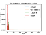
Real-world networks. The networks we use (labeled as RN) are shown in Table 3 with their features ( will be defined later). We use the 130bit network, the econ-mahindas network ((Rossi and Ahmed 2015)), the ego-Facebook network ((Leskovec and Mcauley 2012)), and the email-Eu-core temporal network ((Paranjape, Benson, and Leskovec 2017)). The last two networks are also in Leskovec and Krevl (2014).
| Network | Nodes | Edges | ||
| ego-Facebook | 4039 | 88234 | 27% | 24% |
| Econ | 1258 | 7620 | 6.6% | 1.3% |
| Email-Eu | 986 | 16064 | 30% | 21% |
| 130bit | 584 | 6067 | 41% | 36% |
Our results are summarized below.
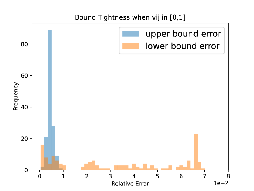
Distribution of samples (Theorem 5). We set the uniform influence factor , showing how the sample assignment is related to degrees at the solution of Equation B.2 on different kinds of networks: scale-free (Figures 1(a) and 1(b)), Erdos-Renyi random networks (Figures 1(c) and 1(d)), and real-world networks (Figures 1(e) and 1(f)). Figures 1(a), 1(c), 1(e) show the average number of samples (divided by ) for each degree; Figure 1(b), 1(d) and 1(f) show the variance of sample number for each degree.
Our main observations are: (1) The samples assigned to nodes with the same degree tend to be almost the same (i.e., the variance is small), (2) Fewer samples tend to be assigned to high-degree agents. These observations are consistent with Theorem 5, which states that sample assignment has negative correlation with degree.
Tightness of bounds (Theorem 7). We empirically show the performance of the bounds in Theorem 7. Here, all influence factors s are generated randomly from . For each kind of synthetic network, we generate 150 different instances with different number of nodes and s. We meausure the performance of bounds in Theorem 7 by relative error (i.e where is the upper bound in Theorem 7 and is the max of (trivial lower bound) and the lower bound in Theorem 7). We visualize the relative error through frequency distributions of generated networks. Our observation is that the bounds are very tight for scale-free graphs (Figure 2(a)), Erdos-Renyi random graphs (Figure 2(b)), and random d-regular graphs (Figure 2(c)).


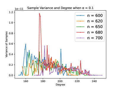


For real-world networks, we generate 50 different and denote the maximum relative error of upper/lower bounds as . From Table 3, the relative errors are still relatively small for real-world networks, showing the tightness of our bounds.
Network Gain (Table 2 and Lemma 17). We empirically demonstrate the network gain results for random -regular graphs (Lemma 17). To calculate the network gain, we replace the in network gain (Equation 1) by its upper bound . This allows us to calculate a lower bound of the network gain, which aligns with the trend of lower bound in Lemma 17. We set and , making . Additionally, we set and consider degree ranging from to . We choose different number of nodes such that degree , which implies a gain in theory (4th row of Table 2 and Lemma 17). The empirical result, shown in Figure 3, exactly confirms the gain is in our setup. Moreover, we also found that when degree , the gain becomes infinity. This is because . According to the 4th row of Table 2 (Lemma 17), in this scenario, it is sufficient for each node to have samples, resulting in an infinite network gain.

6 Discussion and future work
We initiate a study on the total sample complexity (TSC) required for opinion formation over networks. By extending the standard opinion formation game into a machine-learning framework, we characterize the minimal samples needed to ensure low generalization error for equilibrium models. We provide tight bounds on TSC and analyze sample distributions, showing that network structure significantly reduces TSC, with an inverse relationship to node degree being an interesting result.
Our formulation opens several research directions. We currently focus on (generalized) linear regression, but it’s worth investigating if other problems like kernel methods or soft SVMs. Moreover, it turns out that our problem formulation is similar to the best arm identification problem for multi-armed bandits with fixed confidence (Karnin, Koren, and Somekh 2013). It is interesting to extend our results analog to the fixed budget setting. Namely, assuming the number of samples is fixed, how to assign them to minimize the total error? Another future direction is to consider individual-level incentives for sample collection, building on the results of (Blum et al. 2021).
Acknowledgments
RR and OW were partially supported by NSF grant CCF-2335187. AV was partially supported by NSF grants CCF-1918656, IIS-1955797, CNS 2317193 and IIS 2331315. RS was partially supported by NSF grant D-ISN 2146502.
References
- Acemoglu, Chernozhukov, and Yildiz (2006) Acemoglu, D.; Chernozhukov, V.; and Yildiz, M. 2006. Learning and disagreement in an uncertain world.
- Acemoglu and Ozdaglar (2011) Acemoglu, D.; and Ozdaglar, A. 2011. Opinion dynamics and learning in social networks. Dynamic Games and Applications, 1(1): 3–49.
- Andersen et al. (2013) Andersen, M. S.; Dahl, J.; Vandenberghe, L.; et al. 2013. CVXOPT: A Python package for convex optimization. abel. ee. ucla. edu/cvxopt, 88.
- Anderson et al. (1958) Anderson, T. W.; Anderson, T. W.; Anderson, T. W.; and Anderson, T. W. 1958. An introduction to multivariate statistical analysis, volume 2. Wiley New York.
- Audibert and Catoni (2010) Audibert, J.-Y.; and Catoni, O. 2010. Linear regression through PAC-Bayesian truncation. arXiv preprint arXiv:1010.0072.
- Banerjee (1992) Banerjee, A. V. 1992. A simple model of herd behavior. The quarterly journal of economics, 107(3): 797–817.
- Barabási and Albert (1999) Barabási, A.-L.; and Albert, R. 1999. Emergence of scaling in random networks. science, 286(5439): 509–512.
- Bikhchandani, Hirshleifer, and Welch (1992) Bikhchandani, S.; Hirshleifer, D.; and Welch, I. 1992. A theory of fads, fashion, custom, and cultural change as informational cascades. Journal of political Economy, 100(5): 992–1026.
- Bindel, Kleinberg, and Oren (2015) Bindel, D.; Kleinberg, J.; and Oren, S. 2015. How bad is forming your own opinion? Games and Economic Behavior, 92: 248–265.
- Blum et al. (2021) Blum, A.; Haghtalab, N.; Phillips, R. L.; and Shao, H. 2021. One for one, or all for all: Equilibria and optimality of collaboration in federated learning. In International Conference on Machine Learning, 1005–1014. PMLR.
- Blum et al. (2017) Blum, A.; Haghtalab, N.; Procaccia, A. D.; and Qiao, M. 2017. Collaborative PAC Learning. In Proceedings of the 31st International Conference on Neural Information Processing Systems, NIPS’17, 2389–2398. Red Hook, NY, USA: Curran Associates Inc. ISBN 9781510860964.
- Boyd, Boyd, and Vandenberghe (2004) Boyd, S.; Boyd, S. P.; and Vandenberghe, L. 2004. Convex optimization, 232–236. Cambridge university press.
- Breiman and Freedman (1983) Breiman, L.; and Freedman, D. 1983. How many variables should be entered in a regression equation? Journal of the American Statistical Association, 78(381): 131–136.
- Chen, Zhang, and Zhou (2018) Chen, J.; Zhang, Q.; and Zhou, Y. 2018. Tight bounds for collaborative pac learning via multiplicative weights. Advances in neural information processing systems, 31.
- DeGroot (1974) DeGroot, M. H. 1974. Reaching a consensus. Journal of the American Statistical association, 69(345): 118–121.
- DeMarzo, Vayanos, and Zwiebel (2003) DeMarzo, P. M.; Vayanos, D.; and Zwiebel, J. 2003. Persuasion bias, social influence, and unidimensional opinions. The Quarterly journal of economics, 118(3): 909–968.
- Donahue and Kleinberg (2021) Donahue, K.; and Kleinberg, J. 2021. Model-sharing games: Analyzing federated learning under voluntary participation. In Proceedings of the AAAI Conference on Artificial Intelligence, volume 35, 5303–5311.
- Friedkin and Johnsen (1990) Friedkin, N. E.; and Johnsen, E. C. 1990. Social influence and opinions. Journal of Mathematical Sociology, 15(3-4): 193–206.
- Friedman (2003) Friedman, J. 2003. A proof of Alon’s second eigenvalue conjecture. In Proceedings of the thirty-fifth annual ACM symposium on Theory of computing, 720–724.
- Golub and Jackson (2008) Golub, B.; and Jackson, M. O. 2008. How homophily affects diffusion and learning in networks. arXiv preprint arXiv:0811.4013.
- Haddadan, Xin, and Gao (2024) Haddadan, S.; Xin, C.; and Gao, J. 2024. Optimally Improving Cooperative Learning in a Social Setting. In International Conference on Machine Learning. PMLR.
- Haghtalab, Jackson, and Procaccia (2021) Haghtalab, N.; Jackson, M. O.; and Procaccia, A. D. 2021. Belief polarization in a complex world: A learning theory perspective. Proceedings of the National Academy of Sciences, 118(19): e2010144118.
- Haghtalab, Jordan, and Zhao (2022) Haghtalab, N.; Jordan, M.; and Zhao, E. 2022. On-demand sampling: Learning optimally from multiple distributions. Advances in Neural Information Processing Systems, 35: 406–419.
- Jackson (2010) Jackson, M. O. 2010. Social and economic networks. Princeton university press.
- Karnin, Koren, and Somekh (2013) Karnin, Z.; Koren, T.; and Somekh, O. 2013. Almost optimal exploration in multi-armed bandits. In International Conference on Machine Learning, 1238–1246. PMLR.
- Kempe, Kleinberg, and Tardos (2003) Kempe, D.; Kleinberg, J.; and Tardos, E. 2003. Maximizing the Spread of Influence through a Social Network. In Proceedings of the Ninth ACM SIGKDD International Conference on Knowledge Discovery and Data Mining, KDD ’03, 137–146. New York, NY, USA: Association for Computing Machinery. ISBN 1581137370.
- Koltchinskii and Mendelson (2015) Koltchinskii, V.; and Mendelson, S. 2015. Bounding the smallest singular value of a random matrix without concentration. International Mathematics Research Notices, 2015(23): 12991–13008.
- Lalitha et al. (2019) Lalitha, A.; Kilinc, O. C.; Javidi, T.; and Koushanfar, F. 2019. Peer-to-peer federated learning on graphs. arXiv preprint arXiv:1901.11173.
- Lalitha et al. (2018) Lalitha, A.; Shekhar, S.; Javidi, T.; and Koushanfar, F. 2018. Fully decentralized federated learning. In Third workshop on Bayesian Deep Learning (NeurIPS).
- Lecué and Mendelson (2016) Lecué, G.; and Mendelson, S. 2016. Performance of empirical risk minimization in linear aggregation.
- Leskovec and Krevl (2014) Leskovec, J.; and Krevl, A. 2014. SNAP Datasets: Stanford Large Network Dataset Collection. http://snap.stanford.edu/data.
- Leskovec and Mcauley (2012) Leskovec, J.; and Mcauley, J. 2012. Learning to discover social circles in ego networks. Advances in neural information processing systems, 25.
- Liu et al. (2023) Liu, H.; Rajaraman, R.; Sundaram, R.; Vullikanti, A.; Wasim, O.; and Xu, H. 2023. Sample Complexity of Opinion Formation on Networks. arXiv preprint arXiv:2311.02349.
- McMahan et al. (2017) McMahan, B.; Moore, E.; Ramage, D.; Hampson, S.; and y Arcas, B. A. 2017. Communication-efficient learning of deep networks from decentralized data. In Artificial intelligence and statistics, 1273–1282. PMLR.
- Mendelson (2015) Mendelson, S. 2015. Learning without concentration. Journal of the ACM (JACM), 62(3): 1–25.
- Mourtada (2022) Mourtada, J. 2022. Exact minimax risk for linear least squares, and the lower tail of sample covariance matrices. The Annals of Statistics, 50(4): 2157–2178.
- Nguyen and Zakynthinou (2018) Nguyen, H.; and Zakynthinou, L. 2018. Improved algorithms for collaborative PAC learning. Advances in Neural Information Processing Systems, 31.
- Paranjape, Benson, and Leskovec (2017) Paranjape, A.; Benson, A. R.; and Leskovec, J. 2017. Motifs in temporal networks. In Proceedings of the tenth ACM international conference on web search and data mining, 601–610.
- Rossi and Ahmed (2015) Rossi, R. A.; and Ahmed, N. K. 2015. The Network Data Repository with Interactive Graph Analytics and Visualization. In AAAI.
- Rudelson and Vershynin (2015) Rudelson, M.; and Vershynin, R. 2015. Small ball probabilities for linear images of high-dimensional distributions. International Mathematics Research Notices, 2015(19): 9594–9617.
- Simon (2013) Simon, H. A. 2013. Administrative behavior. Simon and Schuster.
- Smith and Sørensen (2000) Smith, L.; and Sørensen, P. 2000. Pathological outcomes of observational learning. Econometrica, 68(2): 371–398.
- Spielman (2019) Spielman, D. A. 2019. Spectral and Algebraic Graph Theory Incomplete Draft, dated December 4, 2019.
- Vanhaesebrouck, Bellet, and Tommasi (2017) Vanhaesebrouck, P.; Bellet, A.; and Tommasi, M. 2017. Decentralized Collaborative Learning of Personalized Models over Networks. In Singh, A.; and Zhu, X. J., eds., Proceedings of the 20th International Conference on Artificial Intelligence and Statistics, AISTATS 2017, 20-22 April 2017, Fort Lauderdale, FL, USA, volume 54 of Proceedings of Machine Learning Research, 509–517. PMLR.
- Young (2014) Young, D. M. 2014. Iterative solution of large linear systems, 42–44. Elsevier.
[section] \printcontents[section]l1
Appendix A Additional details on preliminaries
| Data distribution | |
| Dimension of | |
| Set of samples for agent ; | |
| Number of samples for agent | |
| Initial model for agent (also known as “internal opinion”) | |
| Model learned by agent in opinion formation game | |
| Set of neighbors and degree of node , respectively | |
| Model for agent in the Nash equilibrium | |
| Minimum number of samples that any agent would need to ensure that the best model learned using only their samples ensures that the expected error is at most some target (bounded in Theorem 2 for linear regression) | |
| We denote for all to simplify notations. | |
| We denote for all . |
Appendix B Missing proof in Section 2
B.1 Missing proof in Section 2
Lemma 1. The unique Nash equilibrium of the above game is where and . When all , . Furthermore, we have and for all .
Proof.
For any agent , given , by setting the gradient of the loss function to zero, we have the best response for is . An action profile is a Nash equilibrium if and only if for any , , which is equivalent to for any . Combining all these equations, we have where Note that where is the weighted Laplacian matrix of the graph and is the identity matrix. Since is positive semi-definite, is positive definite. Thus is invertible and . Given the graph structure, is unique and thus the Nash equilibrium is unique. When all , we can simplify by direct calculation.
Since , every non-diagonal element in is negative. On the other hand, since where is the weighted Laplacian matrix of , is symmetric and positive definite. Thus is a Stieltjes matrix. From Young (2014), the inverse of any Stieltjes matrix is a non-negative matrix. Thus, is a non-negative matrix.
Let be the vector in which all elements are . Since , we have . Thus, for any and . Since the best response update for is , the final weight if and only if and are not connected. Since we consider a connected network(or we can consider different connected components separately), we have . Thus, s are normalized weights. ∎
B.2 Missing proofs in Section 3.1
We consider a slightly general case here, where every agent ’s dataset has samples, where are independently drawn from distribution . We assume there is a global ground-truth model such that where is an unbiased noise with bounded variance . We further assume has linear structure over , which means . This capture the case of generalized linear regression (Audibert and Catoni 2010) where and is an arbitrary mapping function.
We further assume every agent learns a unbiased estimator from their dataset such that . Note that in ordinary linear regression is an unbiased estimator. In generalized linear regression, is unbiased where .
We extend the definition of as follows.
Theorem 3. If Assumption 1 holds, then for every agent ,
where and matrix is defined in Lemma 1. Moreover, if we consider linear regression and the condition in Theorem 2 holds, we have
Proof.
To simplify notation, we define in our proof. By Lemma 1, we have and for all . For any agent and any noise , we have
| ( is linear for ) | |||
| () | |||
| ( are unbiased estimators) |
Thus, we have
| (independece of noises) | ||||
For linear regression and the given condition in Theorem 2, we directly have
Note that we can also get the counterpart of Theorem 2 for generalized linear regression. The only thing we need to change is that Assumption 1 and Assumption 2 should be taken for the distribution of rather than . ∎
Theorem 4. For any , let denote an optimal solution of the following optimization problem as a measure of the minimum samples for opinion formation on graph with influence factor .
| s.t. | |||
where is defined in Lemma 1. Then, . Moreover, given and , is a fixed value for any and . If for every , then .
Proof.
We first show a tight characterization of TSC. By Theorem 3, there exists constant such that
| (4) |
By definition, is the solution of Equation 5
| s.t. | (5) | |||
We consider the following two optimizations. Denote the solution of Equation 6 as and the solution of Equation 7 as .
| s.t. | (6) | |||
| s.t. | (7) | |||
From Equation 4, we have
| (8) |
We restate Equation B.2 here and denote the solution as for every .
| s.t. | |||
By defining , Equation B.2 could be reformulated to
| s.t. | (9) | |||
Thus, is a fixed value for any , . This also implies that if is replaced by for some constant in Equation B.2, the solution will become . Thus,
| (10) |
Since , we have
| (11) |
On the other hand, since is always a solution of Equation 7, we have
| (12) |
Combing Equation 8, Equation 10, and Equation 11, we have . Assigning samples to every agent ensures .
If for every , then and . Thus, . From experiments in Section 5, we can observe that for many networks, , thus, setting suffices for in these networks.
∎
Appendix C Missing proof in Section 4.1
C.1 Dual form of Equation B.2
Lemma 9.
Proof.
The Lagrangian of optimization Equation B.2 is
in domain . When for all , we have . When , from , the Lagrangian function gets mininum value when . Now
Thus when , the maxmin problem of Lagrangian is
| s.t. |
Note that when all , this optimization is which matches the infimum of the Lagrangian function when all . Thus we can remove the constraint . The dual problem of optimization Equation B.2 is:
| s.t. |
Since both the objective function and the feasible region of Equation B.2 is convex, following the Slater condition (Boyd, Boyd, and Vandenberghe 2004), strong duality holds because there is a point that strictly satisfies all constraints. ∎
C.2 Proof of Theorem 5
To simplify notations, assume for all . We will first list more observations related to .
Observation 10.
.
Proof.
From , we have . From , we have , which is equivalent to . On the other hand, , . Thus ∎
Observation 11.
for .
Proof.
From , we have . Combining with , we have . Similarly, we get . Since , we have . ∎
We restate Theorem 5 and prove it here.
Theorem 5. The optimal solution to Equation B.2 satisfies
Assigning samples to node can make sure at the equilibrium, every agent has error . Assigning samples to node is sufficent to solve the TSC problem.
Proof.
(1) For the upper bound, let . Equation B.2 then becomes
| s.t. | |||
The optimal solution is when . From Observation 10 and Observation 11,
Note that this bound holds for all , thus we have
Thus, . Since is a solution of Equation B.2, assign samples to to node can make sure at the equilibrium, every agent has error . Assigning samples to node is sufficent to solve the TSC problem.
(2) For the lower bound, we utilize the dual form Equation 13. Let where will be optimized later. The dual optimization then becomes
| s.t. |
Let be the solution of this optimization given . Since the objective function is a quadratic function, the function gets maximal value when
Thus,
From Observation 10, we have , thus
Note that this holds for all , to get the tightest bound, we should find the maximal value of the last term. By Cauchy–Schwarz inequality, we have
This maximum value is achieved when . Thus .
(3) In the dual form Equation 13, for any is a feasible solution. From strong duality, we have
| (Cauchy-Schwarz) | ||||
| ( for all ) |
∎
C.3 Bounds for the Network Gain
From Theorem 2, for every agent , we have
| (14) |
Recall that is the minimal number of samples one agent needs to learn a model with error. We have
| (15) |
By Theorem 3, we have
| (16) |
Corollary 6. For any network , if , then . If , then .
Proof.
We first derive the upper bound of the network gain. From Equation 16, Equation 8, and Equation 12, we have
This implies
where the last step applies the upper bound in Theorem 5. The assumption implies for every , and . We have
We now derive a general upper bound of the network gain. From Equation 16, Equation 8, and Equation 10, we have
This implies
| (17) |
where the last step applies the lower bound in Theorem 5. The assumption is equivalent to for every . This implies which leads to
When , we have , thus, . When , , this implies . We have
where we use the trivial lower bound in Theorem 5. Thus, . ∎
We then consider another lower bound of network gain, which will be applied to prove the network gain for special networks.
Lemma 12.
Let be a feasible solution of Equation B.2. If , the network gain is infinite. If , we have
C.4 Proof of Network Gain for Special Networks
Again, To simplify notations, assume for all .
Lemma 13.
If the network is an -clique, , where for every . The network gain
Proof.
For n-clique, we have . The solution to this system is for any . Thus for any , . Since the constraints of Equation B.2 are symmetric now, there is an optimal solution such that . The constraint now becomes . Thus the unique optimal solution is when .
Lemma 14.
For an -agent star graph, . If , the network gain .
Proof.
Recall the optimization problem in Theorem 4. To get a lower bound on any , we upper bound the quantity for any . The key idea is to investigate the structure of . Since is a symmetric positive definite matrix when the influence factors have uniform value , it can be written in terms of its eigen-decomposition as where is an orthonormal matrix whose columns are unit eigenvectors of s.t. for any , , and is the diagonal matrix of the corresponding eigenvalues of . Let denote the eigenvalues of the Laplacian matrix of such that . By definition of , it follows that the eigenvalues of can be expressed as . It is well known that for any graph, and for -regular graphs, the eigenvalues . Furthermore, note that so that . Another observation we make is that the eigenvectors of are simply the eigenvectors of the Laplacian .
Similarly, we express in terms of its eigen-decomposition. Since , it follows that where is the diagonal matrix such that for all . To lower bound any entry of , it suffices to compute the eigenvalues and eigenvectors of the Laplacian matrix . Based on the above observations, we have,
where denotes the -entry of the eigenvector . This implies that
where denotes the matrix . The last equality follows from the fact that is symmetric. Now, note that so that, .
Effectively, to bound , we upper bound the quantity which depends only on , eigenvalues and eigenvectors of the graph Laplacian , summarized in the following Lemma.
Lemma 15.
. Moreover, for every is a feasible solution to Equation B.2.
Proof.
Lemma 16.
Consider a graph which is a -dimensional hypercube where , and is a power of . Then, when is a constant with , . The network gain . Assigning samples to every agent suffices to solve the TSC problem.
Proof.
It is known that for the hypercube, it holds that for all eigenvectors , and all , and eigenvalues of are given by for with multiplicity respectively (Spielman 2019). Based on this, we have that for any ,
We bound the quantity, . For this purpose, we look at the quantity where will be set later. Now,
Integrating over and setting we get that,
Assuming , we get,
It follows that,
so that,
Note that this holds for all . Thus, by Lemma 15, we get that is a feasible solution to Equation B.2, and . On the other hand, from the lower bound in Theorem 5, we have . Since , we have . Since is a feasible solution to Equation B.2. Assigning samples to every agent is sufficent to solve the TSC problem. By Lemma 12, we have
∎
Lemma 17.
For a random -regular graph, with probability of at least where
(1) If , . Assigning samples to every agent suffices to solve the TSC problem. The network gain .
(2) If , . Assigning suffices to solve the TSC problem. The network gain .
Proof.
For a random -regular graph, it is known that the largest eigenvalue of the adjacency matrix is and with the probability of at least where , the rest of the eigenvalues are in the range (Friedman 2003). This implies that for the Laplacian the smallest eigenvalue is and the rest of the eigenvalues are . Since in the Laplacian matrix, for all . We have that, for every ,
Lemma 18.
Consider a graph which is a -regular expander with expansion . Then, we have that
(1) When , then . Assigning samples to every agent suffices to solve the TSC problem. The network gain .
(2) When , then . Assigning samples to every agent suffices to solve the TSC problem. The network gain .
Proof.
Since for any graph, we know from Cheeger’s inequality that the second smallest eigenvalue satisfies,
from which it follows that . Then, we have that
Note that this holds for all . Thus, by Lemma 15, , and is a feasible solution to Equation B.2. Thus, when , . Since now, assigning samples to every agent suffices to solve the TSC problem. The network gain .
When , . Since now, assigning samples to every agent suffices to solve the TSC problem. The network gain . ∎
Appendix D Missing proof in Section 4.2
To simplify notations, assume for all . Since is positive-definite, from the Schur product theorem, is also positive-definite where is the Hadamard product (element-wise product). Let and .
Lemma 19.
for all
Proof.
Let , we have . Let be the adjoint matrix of respectively. We have . Consider the sum of the row of , to prove it is positive, since is positive, we only need to prove the sum of the row of is positive. The -row sum of is where is generated by replacing the row of to all one vector. Similarly, we can define . Since is positive definite, the first leading principal minors of , which are exactly the same as , are positive. On the other hand, . Thus, is positive definite. Note that , from Schur product theorem, is positive definite. Thus , which means . By relabeling each node to , we can get for all . ∎
Proof.
From Lemma 9, strong duality holds. Thus, we can only consider the solution of dual form.
| s.t. |
Let be the objective function of Equation 13 Setting gradient to zero, we have for any . Let , we have . The matrix here is equivalent to where denotes the Hadamard product of two matrices. Since is positive definite, is also positive definite. From Schur product theorem, is positive definite and then is invertible. Since and , we have . In Lemma 19, we have shown that , thus, this solution is valid. Considering , we have for any . Thus . We have (Note that it can be negative). This solution is valid if and only if for any . If this solution is valid, the optimal solution is:
From KKT conditions, setting the gradient of the Lagrangian function of (P) to zero, we have
where is the element on the -th row and -th column of identity matrix . The fourth equality comes from where the . ∎
Theorem 7. Let for every , then we have
Assigning samples to node suffices to solve the TSC problem.
Proof.
(1) is trivial because for any is a feasible solution for the Equation B.2 because for any
(2) Let , . In Equation B.2, setting the first constraints to equality for every , we have . From Lemma 19, the solution is feasible (). Now , , and . Since is in the feasible region, . Thus, . Assigning samples to node suffies to solve the TSC problem.
(3) In the dual form Equation 13, for any is a feasible solution. From strong duality, we have
| (Cauchy-Schwarz) | ||||
| ( for all ) |
Appendix E Missing proof in Section 5
Lemma 20.
The optimization Equation B.2 is equivalent to the following second-order cone programming.
| s.t. | |||
The optimal solution is equal to the optimal solution in the optimization (P).
Proof.
The original optimization Equation B.2 is :
| s.t. | |||
Let and , the programming is equivalent to
| s.t. | |||
The constraint is equivalent to . Thus, this programming is equivalent to the following second-order cone programming.
| s.t. | |||
∎
Appendix F More Experiments
In this section, we will give more detailed experiments. Our code can be found in https://github.com/liuhl2000/Sample-Complexity-of-Opinion-Formation-on-Networks. These experiments are done with seven 8-core Intel CPUs. The optimization is solved by running the solver until the convergence error is less than . All optimizations for our chosen networks could be finished in 150 iterations. The most time-consuming part is generating random weights 50 times and running corresponding experiments in Section F.2. Actually, there is little difference among these random experiments and in order to reproduce our experiments quickly, you can simply set the “Iter num” parameter to in our code.
F.1 Distribution of Samples at the Optimal Point
To study the distribution of samples, we assume all . In our experiments, we choose . For figures in this section, the x-axis is node degree and the y-axis is the average or variance of where is the sample assigned to agent at the optimal point of Equation B.2.
We generate scale-free networks using Barabasi–Albert preferential attachment (Barabási and Albert 1999) with attachment parameter (Incoming node will attach to two existing nodes) for . Figure 4 and Figure 5 show the average sample number and variance for different .


We use Erdos-Renyi random networks with probability (Two nodes has the probability to have one edge) for . Figure 6 and Figure 7 show the average sample number and variance for different .


For real-world networks, Figure 8, 9, and Figure 10 show the average sample number and variance for different .


Based on the above results, low-degree agents tend to have more samples, and agents with the same degree tend to have the same number of samples. When is small, the sample assignment seems to have relatively good monotonicity with but as gets larger, the trend for high degrees becomes more unpredictable.
Another observation is that as increases, the samples assigned to each degree decrease when gets larger. Our theory can not explain this well now, and it is interesting to investigate it more in future work.
F.2 Tightness of bounds
In this section, we test the tightness of our upper and lower bound in Theorem 7. We also study the impact of the magnitude of influences factors on the performance of bounds. The influence factors s are uniformly generated at random from .
Our synthesized graphs are generated for . For each , we generate networks with different structures and s (The detailed process will be discussed later). For all these networks, we calculate their optimal solution, the upper bound and the lower bound indicated in Theorem 7. We measure the performance of bounds in Theorem 7 by relative error (i.e where is the upper in Theorem 7) and is the max of 1 and the lower bound in Theorem 7. In the following plots, the x-axis is the relative errors of upper/lower bounds and the y-axis is the frequency (number of networks in each bin).
For scale-free networks, for each , we randomly generate networks with attachment parameter and networks with attachment parameter . The influence factors of these networks are also randomly generated in a given range. The error plot is given in Figure 11.


For random regular graphs, for each , we generate graphs with degree roughly equal to where . For each degree, we generate graphs. The influence factors of these networks are also randomly generated in a given range. The error is given in Figure 12.


For Erdos-Renyi graphs, for each , we generate graphs with edge-connection probability . The influence factors of these networks are also randomly generated in a given range. The error plot is given in Figure 13.


In Table 5, we show the relative error for bounds of different real-world networks for different s. Let and be the maximum relative error of the upper and lower bound in Theorem 7 respectively among these random experiments.
| Network | Upper bound of | ||
| ego-Facebook | 0.01 | ||
| ego-Facebook | 0.1 | ||
| ego-Facebook | 1 | ||
| ego-Facebook | 5 | ||
| ego-Facebook | 10 | ||
| Econ | 0.01 | ||
| Econ | 0.1 | ||
| Econ | 1 | ||
| Econ | 5 | ||
| Econ | 10 | ||
| Email-Eu | 0.01 | ||
| Email-Eu | 0.1 | ||
| Email-Eu | 1 | ||
| Email-Eu | 5 | ||
| Email-Eu | 10 | ||
| 130bit | 0.01 | ||
| 130bit | 0.1 | ||
| 130bit | 1 | ||
| 130bit | 5 | ||
| 130bit | 10 |
From all experiments above, we can observe that the performance of the bounds in Theorem 7 is excellent when the influence factors are small but get worse when the influence factors become larger.
The reason why these two bounds get good performance for small influence factors has the following intuitive explanation. Consider the original optimization Equation B.2, when all influence factors are zero, the optimal value is achieved when we set all inequality of the first constraint to equality. When influence factors are small, the optimal solution will also tend to be the value derived in this way, which is exactly the method we get our upper and lower bound.
Through all these experiments, an obvious result is that when gets large, the total sample complexity decreases. However, our upper bound in Theorem 5, by assigning each agent , does not capture this trend. It seems that we can remove the in the numerator to improve this bound and we leave it as future work.