SAM operates far from home: eigenvalue regularization as a dynamical phenomenon
Abstract
The Sharpness Aware Minimization (SAM) optimization algorithm has been shown to control large eigenvalues of the loss Hessian and provide generalization benefits in a variety of settings. The original motivation for SAM was a modified loss function which penalized sharp minima; subsequent analyses have also focused on the behavior near minima. However, our work reveals that SAM provides a strong regularization of the eigenvalues throughout the learning trajectory. We show that in a simplified setting, SAM dynamically induces a stabilization related to the edge of stability (EOS) phenomenon observed in large learning rate gradient descent. Our theory predicts the largest eigenvalue as a function of the learning rate and SAM radius parameters. Finally, we show that practical models can also exhibit this EOS stabilization, and that understanding SAM must account for these dynamics far away from any minima.
1 Introduction
Since the dawn of optimization, much effort has gone into developing algorithms which use geometric information about the loss landscape to make optimization more efficient and stable (Nocedal, 1980; Duchi et al., 2011; Lewis & Overton, 2013). In more modern machine learning, control of the large curvature eigenvalues of the loss landscape has been a goal in and of itself (Hochreiter & Schmidhuber, 1997; Chaudhari et al., 2019). There is empirical and theoretical evidence that controlling curvature of the training landscape leads to benefits for generalization (Keskar et al., 2017; Neyshabur et al., 2017), although in general the relationship between the two is complex (Dinh et al., 2017).
Recently the sharpness aware minimization (SAM) algorithm has emerged as a popular choice for regularizing the curvature during training (Foret et al., 2022). SAM has the advantage of being a tractable first-order method; for the cost of a single extra gradient evaluation, SAM can control the large eigenvalues of the loss Hessian and often leads to improved optimization and generalization (Bahri et al., 2022).
However, understanding the mechanisms behind the effectiveness of SAM is an open question. The SAM algorithm itself is a first-order approximation of SGD on a modified loss function . Part of the original motivation was that explicitly penalizes sharp minima over flatter ones. However the approximation performs as well or better than running gradient descent on directly. SAM often works better with small batch sizes as compared to larger ones (Foret et al., 2022; Andriushchenko & Flammarion, 2022).These stochastic effects suggest that studying the deterministic gradient flow dynamics on will not capture key features of SAM, since small batch size induces non-trivial differences from gradient flow (Paquette et al., 2021).
In parallel to the development of SAM, experimental and theoretical work has uncovered some of the curvature-controlling properties of first-order methods due to finite step size - particularly in the full batch setting. At intermediate learning rates, a wide variety of models and optimizers show a tendency for the largest Hessian eigenvalues to stabilize near the edge of stability (EOS) for long times (Lewkowycz et al., 2020; Cohen et al., 2022a, b). The EOS is the largest eigenvalue which would lead to convergence for a quadratic loss landscape. This effect can be explained in terms of a non-linear feedback between the large eigenvalue and changes in the parameters in that eigendirection (Damian et al., 2022; Agarwala et al., 2022).
We will show that these two areas of research are in fact intimately linked: under a variety of conditions, SAM displays a modified EOS behavior, which leads to stabilization of the largest eigenvalues at a lower magnitude via non-linear, discrete dynamics. These effects highlight the dynamical nature of eigenvalue regularization, and demonstrates that SAM can have strong effects throughout a training trajectory.
1.1 Related work
Previous experimental work suggested that decreasing batch size causes SAM to display both stronger regularization and better generalization (Andriushchenko & Flammarion, 2022). This analysis also suggested that SAM may induce more sparsity.
A recent theoretical approach studied SAM close to a minimum, where the trajectory oscillates about the minima and provably decreases the largest eigenvalue (Bartlett et al., 2022). A contemporaneous approach studied the SAM algorithm in the limit of small learning rate and SAM radius, and quantified how the implicit and explicit regularization of SAM differs between full batch and batch size dynamics (Wen et al., 2023).
1.2 Our contributions
In contrast to other theoretical approaches, we study the behavior of SAM far from minima. We find that SAM regularizes the eigenvalues throughout training through a dynamical phenomenon and analysis only near convergence cannot capture the full picture. In particular, in simplified models we show:
-
•
Near initialization, full batch SAM provides limited suppression of large eigenvalues (Theorem 2.1).
-
•
SAM induces a modified edge of stability (EOS) (Theorem 2.2).
-
•
For full batch training, the largest eigenvalues stabilize at the SAM-EOS, at a smaller value than pure gradient descent (Section 3).
-
•
As batch size decreases, the effect of SAM is stronger and the dynamics is no longer controlled by the Hessian alone (Theorem 2.3).
We then present experimental results on realistic models which show:
-
•
The SAM-EOS predicts the largest eigenvalue for WideResnet 28-10 on CIFAR10.
Taken together, our results suggest that SAM can operate throughout the learning trajectory, far from minima, and that it can use non-linear, discrete dynamical effects to stabilize large curvatures of the loss function.
2 Quadratic regression model
2.1 Basic model
We consider a quadratic regression model (Agarwala et al., 2022) which extends a linear regression model to second order in the parameters. Given a -dimensional parameter vector , the -dimensional output is given by :
| (1) |
Here, is a -dimensional vector, is a -dimensional matrix, and is a - dimensional tensor symmetric in the last two indices - that is, takes two -dimensional vectors as input, and outputs a -dimensional vector . If , the model corresponds to linear regression. , , and are all fixed at initialization.
Consider optimizing the model with under a squared loss. More concretely, let be a -dimensional vector of training targets. We focus on the MSE loss
| (2) |
We can write the dynamics in terms of the residuals and the Jacobian defined by
| (3) |
The loss can be written as . The full batch gradient descent (GD) dynamics of the parameters are given by
| (4) |
which leads to
| (5) |
The -dimensional matrix is known as the neural tangent kernel (NTK) (Jacot et al., 2018), and controls the dynamics for small (Lee et al., 2019).
We now consider the dynamics of un-normalized SAM (Andriushchenko & Flammarion, 2022). That is, given a loss function we study the update rule
| (6) |
We are particularly interested in small learning rate and small SAM radius. The dynamics in space are given by
| (7) |
| (8) |
to lowest order in and .
From Equation 7 we see that for small and , the dynamics of is controlled by the modified NTK . The factor shows up in the dynamics of as well, and we will show that this effective NTK can lead to dynamical stabilization of large eigenvalues. And note that when , these dynamics coincide with that of gradient descent.
2.2 Gradient descent theory
2.2.1 Eigenvalue dynamics at initialization
A basic question is: how does SAM affect the eigenvalues of the NTK? We can study this directly for early learning dynamics by using random initializations. We have the following theorem (proof in Appendix A.2):
Theorem 2.1.
Consider a second-order regression model, with initialized randomly with i.i.d. components with mean and variance . For a model trained with full batch gradient descent, with unnormalized SAM, the change in at the first step of the dynamics, averaged over is
| (9) |
The th singular value of associated with left and right singular vectors and can be approximated as
| (10) |
for small .
Note that the singular vector is an eigenvector of associated with the eigenvalue .
This analysis suggests that on average, at early times, the change in the singular value is negative. However, the change also depends linearly on . This suggests that if the component of in the direction of the singular vector becomes small, the stabilizing effect of SAM becomes small as well. For large batch size/small learning rate with MSE loss, we in fact expect to decrease rapidly early in training (Cohen et al., 2022a; Agarwala et al., 2022). Therefore the relative regularizing effect can be weaker for larger modes in the GD setting.

 |
 |
 |
2.2.2 Edge of stability and SAM
One of the most dramatic consequences of SAM for full batch training is the shift of the edge of stability. We begin by reviewing the EOS phenomenology. Consider full-batch gradient descent training with respect to a twice-differentiable loss. Near a minimum of the loss, the dynamics of the displacement from the minimum (in parameter space) are well-approximated by
| (11) |
where is the positive semi-definite Hessian at the minimum . The dynamics converges exponentially iff the largest eigenvalue of is bounded by . We refer to as the normalized eigenvalue, Otherwise, there is at least one component of which is non-decreasing. The value is often referred to as the edge of stability (EOS) for the dynamics.
Previous work has shown that for many non-linear models, there is a range of learning rates where the largest eigenvalue of the Hessian stabilizes around the edge of stability (Cohen et al., 2022a). Equivalent phenomenology exists for other gradient-based methods (Cohen et al., 2022b). The stabilization effect is due to feedback between the largest curvature eigenvalue and the displacement in the largest eigendirection (Agarwala et al., 2022; Damian et al., 2022). For MSE loss, EOS behavior occurs for the large NTK eigenvalues as well (Agarwala et al., 2022).
We will show that SAM also induces an EOS stabilization effect, but at a smaller eigenvalue than GD. We can understand the shift intuitively by analyzing un-normalized SAM on a loss . Direct calculation gives the update rule:
| (12) |
For positive definite , converges exponentially to iff . Recall from Section 2.1 that the SAM NTK is . This suggests that is the SAM normalized eigenvalue. This bound gives a critical which is smaller than that in the GD case. This leads to the hypothesis that SAM can cause a stabilization at the EOS in a flatter region of the loss, as schematically illustrated in Figure 1.
We can formalize the SAM edge of stability (SAM EOS) for any differentiable model trained on MSE loss. Equation 7 suggests the matrix - which has larger eigenvalues for larger - controls the low-order dynamics. We can formalize this intuition in the following theorem (proof in Appendix B.1):
Theorem 2.2.
Consider a model trained using Equation 6 with MSE loss. Suppose that there exists a point where . Suppose that for some , we have the lower bound for the eigenvalues of the positive definite symmetric matrix . Given a bound on the largest eigenvalue, there are two regimes:
Convergent regime. If for all for all eigenvalues of , there exists a neighborhood of such that with exponential convergence for any trajectory initialized at .
Divergent regime. If for some eigenvector of , then there exists some such that for any , given , the ball of radius around , there exists some initialization such that the trajectory leaves at some time .
Note that the theorem is proven for the NTK eigenvalues, which also show EOS behavior for MSE loss in the GD setting (Agarwala et al., 2022).
This theorem gives us the modified edge of stability condition:
| (13) |
For larger , a smaller is needed to meet the edge of stability condition. In terms of the normalized eigenvalue , the modified EOS can be written as with the ratio . Larger values of lead to stronger regularization effects, and for the quadratic regression model specifically can be factored out leaving as the key dimensionless parameter (Appendix A.1).
2.3 SGD theory
It has been noted that the effects of SAM have a strong dependence on batch size (Andriushchenko & Flammarion, 2022). While a full analysis of SGD is beyond the scope of this work, we can see some evidence of stronger regularization for SGD in the quadratic regression model.
Consider SGD dynamics, where a random fraction of the training residuals are used to generate the dynamics at each step. We can represent the sampling at each step with a random projection matrix , and replacing all instances of with . Under these dynamics, we can can prove the following:
Theorem 2.3.
Consider a second-order regression model, with initialized randomly with i.i.d. components with mean and variance . For a model trained with SGD, sampling datapoints independently at each step, the change in and at the first step, averaged over and the sampling matrix , is given by
| (14) |
| (15) |
where is the batch fraction.
The calculations are detailed in Appendix A.2. This suggests that there are two possible sources of increased regularization for SGD: the first being the additional terms proportional to . In addition to the fact that for , we have
| (16) |
for left and right eigenvectors and of , where is the Hadamard (elementwise) product. This term can be large even if and have small dot product. This is in contrast to , which is small if does not have a large component in the direction. This suggests that at short times, where the large eigenmodes decay quickly, the SGD term can still be large. Additionally, the onto the largest eigenmode itself decreases more slowly in the SGD setting (Paquette et al., 2021), which also suggests stronger early time regularization for small batch size.

3 Experiments on basic models
3.1 Quadratic regression model
We can explore the effects of SAM and show the SAM EOS behavior via numerical experiments on the quadratic regression model. We use the update rule in Equation 6, working directly in and space as in (Agarwala et al., 2022). Experimental details can be found in Appendix A.3.
For small learning rates, we see that SAM does not reduce the large eigenvalues of in the dynamics (Figure 2, left). In fact in some cases the final eigenvalue is larger with SAM turned on. The projection onto the largest eigenmodes of exponentially decreases to quicker than any other mode; as suggested by Theorem 2.1, this leads to only a small decreasing pressure from SAM. The primary dynamics of the large eigenvalues is due to the progressive sharpening phenomenology studied in (Agarwala et al., 2022), which tends to increase the eigenmodes.
However, for larger learning rates, SAM has a strong suppressing effect on the largest eigenvalues (Figure 2, middle). The overall dynamics are more non-linear than in the small learning rate case. The eigenvalues stabilize at the modified EOS boundary (Figure 2, right), suggesting non-linear stabilization of the eigenvalues. In Appendix A.3 we conduct additional experiments which confirm that the boundary predicts the largest eigenvalue for a range of , and that consequently generally increasing leads to decreased .
3.2 CIFAR- with MSE loss
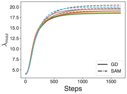
We can see this phenomenology in more general non-linear models as well. We trained a fully-connected network on the first classes of CIFAR with MSE loss, with both full batch gradient descent and SAM. We then computed the largest eigenvalues of along the trajectory. We can see that in both GD and SAM the largest eigenvalues stabilize, and the stabilization threshold is smaller for SAM (Figure 3). The threshold is once again well predicted by the SAM EOS.
4 Connection to realistic models
 |
 |
 |
In this section, we show that our analysis of quadratic models can bring insights into the behavior of more realistic models.
4.1 Setup
Sharpness For MSE loss, edge of stability dynamics can be shown in terms of either the NTK eigenvalues or the Hessian eigenvalues (Agarwala et al., 2022). For more general loss functions, EOS dynamics takes place with respect to the largest Hessian eigenvalues (Cohen et al., 2022a; Damian et al., 2022). Following these results and the analysis in Equation 12, we chose to measure the largest eigenvalue of the Hessian rather than the NTK. We used a Lanczos method (Ghorbani et al., 2019) to approximately compute . Any reference to in this section refers to eigenvalues computed in this way.
CIFAR-10 We conducted experiments on the popular CIFAR-10 dataset (Krizhevsky et al., 2009) using the WideResnet 28-10 architecture (Zagoruyko & Komodakis, 2016). We report results for both the MSE loss and the cross-entropy loss. In the case of the MSE loss, we replace the softmax non-linearity with Tanh and rescale the one-hot labels to . In both cases, the loss is averaged across the number of elements in the batch and the number of classes. For each setting, we report results for a single configuration of the learning rate and weight decay found from an initial cross-validation sweep. For MSE, we use and for cross-entropy. We use the cosine learning rate schedule (Loshchilov & Hutter, 2016) and SGD instead of Nesterov momentum (Sutskever et al., 2013) to better match the theoretical setup. Despite the changes to the optimizer and the loss, the test error for the models remains in a reasonable range (4.4% for SAM regularized models with MSE and 5.3% with SGD). In accordance with the theory, we use unnormalized SAM in these experiments. We keep all other hyper-parameters to the default values described in the original WideResnet paper.
4.2 Results
As shown in Figure 4 (left), the maximum eigenvalue increases significantly throughout training for all approaches considered. However, the normalized curvature , which sets the edge of stability in GD, remains relatively stable early on in training when the learning rate is high, but necessarily decreases as the cosine schedule drives the learning rate to (Figure 4, middle).
SAM radius drives curvature below GD EOS. As we increase the SAM radius, the largest eigenvalue is more controlled (Figure 4, left) - falling below the gradient descent edge of stability (Figure 4, middle). The stabilizing effect of SAM on the large eigenvalues is evident even early on in training.
Eigenvalues stabilize around SAM-EOS. If we instead plot the SAM-normalized eigenvalue , we see that the eigenvalues stay close to (and often slightly above) the critical value of , as predicted by theory (Figure 4, right). This suggests that there are settings where the control that SAM has on the large eigenvalues of the Hessian comes, in part, from a modified EOS stabilization effect.
 |
 |
Altering SAM radius during training can successfully move us between GD-EOS and SAM-EOS. Further evidence from EOS stabilization comes from using a SAM schedule. We trained the model with two settings: early SAM, where SAM is used for the first steps ( epochs), after which the training proceeds with SGD (), and late SAM, where SAM is used for the first steps, after which only SGD is used. The maximum eigenvalue is lower for early SAM before steps, after which there is a quick crossover and late SAM gives better control (Figure 5). Both SAM schedules give improvement over SGD-only training. Generally, turning SAM on later or for the full trajectory gave better generalization than turning SAM on early, consistent with the earlier work of Andriushchenko & Flammarion (2022).
Plotting the eigenvalues for the early SAM and late SAM schedules, we see that when SAM is turned off, the normalized eigenvalues lie above the gradient descent EOS (Figure 5, right, blue curves). However when SAM is turned on, is usually below the edge of stability value of ; instead, the SAM-normalized value lies close to the critical value of (Figure 5, right, orange curves). This suggests that turning SAM on or off during the intermediate part of training causes the dynamics to quickly reach the appropriate edge of stability.
Networks with cross-entropy loss behave similarly. We found similar results for cross-entropy loss as well, which we detail in Appendix C.1. The mini-batch gradient magnitude and eigenvalues vary more over the learning trajectories; this may be related to effects of logit magnitudes which have been previously shown to affect curvature and general training dynamics (Agarwala et al., 2020; Cohen et al., 2022a).
Minibatch gradient norm varies little. Another quantity of interest is the magnitude of the mini-batch gradients. For SGD, the gradient magnitudes were steady during the first half of training and dropped by a factor of at late times (Figure 6). Gradient magnitudes were very stable for SAM, particularly for larger . This suggests that in practice, there may not be much difference between the normalized and un-normalized SAM algorithms. This is consistent with previous work which showed that the generalization of the two approaches is similar (Andriushchenko & Flammarion, 2022).

5 Discussion
5.1 SAM as a dynamical phenomenon
Much like the study of EOS before it, our analysis of SAM suggests that sharpness dynamics near minima are insufficient to capture relevant phenomenology. Our analysis of the quadratic regression model suggests that SAM already regularizes the large eigenmodes at early times, and the EOS analysis shows how SAM can have strong effects even in the large-batch setting. Our theory also suggested that SGD has additional mechanisms to control curvature early on in training as compared to full batch gradient descent.
The SAM schedule experiments provided further evidence that multiple phases of the optimization trajectory are important for understanding the relationship between SAM and generalization. If the important effect was the convergence to a particular minimum, then only late SAM would improve generalization. If instead some form of “basin selection” was key, then only early SAM would improve generalization. The fact that both are important (Andriushchenko & Flammarion, 2022) suggests that the entire optimization trajectory matters.
We note that while EOS effects are necessary to understand some aspects of SAM, they are certainly not sufficient. As shown in Appendix A.3, the details of the behavior near the EOS have a complex dependence on (and the model). Later on in learning, especially with a loss like cross entropy, the largest eigenvalues may decrease even without SAM (Cohen et al., 2022a) - potentially leading the dynamics away from the EOS. Small batch size may add other effects, and EOS effects become harder to understand if multiple eigenvalues are at the EOS. Nonetheless, even in more complicated cases the SAM EOS gives a good approximation to the control SAM has on the eigenvalues, particularly at early times.
5.2 Optimization and regularization are deeply linked
This work provides additional evidence that understanding some regularization methods may in fact require analysis of the optimization dynamics - especially those at early or intermediate times. This is in contrast to approaches which seek to understand learning by characterizing minima, or analyzing behavior near convergence only. A similar phenomenology has been observed in evolutionary dynamics - the basic th order optimization method - where the details of optimization trajectories are often more important than the statistics of the minima to understand long-term dynamics (Nowak & Krug, 2015; Park & Krug, 2016; Agarwala & Fisher, 2019).
6 Future work
Our main theoretical analysis focused on the dynamics and under squared loss; additional complications arise for non-squared losses like cross-entropy. Providing a detailed quantitative characterization of the EOS dynamics under these more general conditions is an important next step.
Another important open question is the analysis of SAM (and the EOS effect more generally) under SGD. While Theorem 2.3 provides some insight into the differences, a full understanding would require an analysis of for the different eigenmodes - which has only recently been analyzed for a quadratic loss function (Paquette et al., 2021, 2022a, 2022b; Lee et al., 2022). Our analysis of the CIFAR10 models showed that the SGD gradient magnitude does not change much over training. Further characterization of the SGD gradient statistics will also be useful in understanding the interaction of SAM and SGD.
More detailed theoretical and experimental analysis of more complex settings may allow for improvements to the SAM algorithm and its implementation in practice. A more detailed theoretical understanding could lead to proposals for -schedules, or improvements to the core algorithm itself - already a field of active research (Zhuang et al., 2022).
Finally, our work focuses on optimization and training dynamics; linking these properties to generalization remains a key goal of any further research into SAM and other optimization methods.
References
- Agarwala & Fisher (2019) Agarwala, A. and Fisher, D. S. Adaptive walks on high-dimensional fitness landscapes and seascapes with distance-dependent statistics. Theoretical Population Biology, 130:13–49, December 2019. ISSN 0040-5809. doi: 10.1016/j.tpb.2019.09.011.
- Agarwala et al. (2020) Agarwala, A., Pennington, J., Dauphin, Y., and Schoenholz, S. Temperature check: Theory and practice for training models with softmax-cross-entropy losses, October 2020.
- Agarwala et al. (2022) Agarwala, A., Pedregosa, F., and Pennington, J. Second-order regression models exhibit progressive sharpening to the edge of stability, October 2022.
- Andriushchenko & Flammarion (2022) Andriushchenko, M. and Flammarion, N. Towards Understanding Sharpness-Aware Minimization, June 2022.
- Bahri et al. (2022) Bahri, D., Mobahi, H., and Tay, Y. Sharpness-Aware Minimization Improves Language Model Generalization, March 2022.
- Bartlett et al. (2022) Bartlett, P. L., Long, P. M., and Bousquet, O. The Dynamics of Sharpness-Aware Minimization: Bouncing Across Ravines and Drifting Towards Wide Minima, October 2022.
- Chaudhari et al. (2019) Chaudhari, P., Choromanska, A., Soatto, S., LeCun, Y., Baldassi, C., Borgs, C., Chayes, J., Sagun, L., and Zecchina, R. Entropy-SGD: Biasing gradient descent into wide valleys. Journal of Statistical Mechanics: Theory and Experiment, 2019(12):124018, December 2019. ISSN 1742-5468. doi: 10.1088/1742-5468/ab39d9.
- Cohen et al. (2022a) Cohen, J., Kaur, S., Li, Y., Kolter, J. Z., and Talwalkar, A. Gradient Descent on Neural Networks Typically Occurs at the Edge of Stability. In International Conference on Learning Representations, February 2022a.
- Cohen et al. (2022b) Cohen, J. M., Ghorbani, B., Krishnan, S., Agarwal, N., Medapati, S., Badura, M., Suo, D., Cardoze, D., Nado, Z., Dahl, G. E., and Gilmer, J. Adaptive Gradient Methods at the Edge of Stability, July 2022b.
- Damian et al. (2022) Damian, A., Nichani, E., and Lee, J. D. Self-Stabilization: The Implicit Bias of Gradient Descent at the Edge of Stability, September 2022.
- Dinh et al. (2017) Dinh, L., Pascanu, R., Bengio, S., and Bengio, Y. Sharp minima can generalize for deep nets. In Proceedings of the 34th International Conference on Machine Learning - Volume 70, ICML’17, pp. 1019–1028, Sydney, NSW, Australia, August 2017. JMLR.org.
- Duchi et al. (2011) Duchi, J., Hazan, E., and Singer, Y. Adaptive Subgradient Methods for Online Learning and Stochastic Optimization. Journal of Machine Learning Research, 12(61):2121–2159, 2011. ISSN 1533-7928.
- Foret et al. (2022) Foret, P., Kleiner, A., Mobahi, H., and Neyshabur, B. Sharpness-aware Minimization for Efficiently Improving Generalization. In International Conference on Learning Representations, April 2022.
- Ghorbani et al. (2019) Ghorbani, B., Krishnan, S., and Xiao, Y. An Investigation into Neural Net Optimization via Hessian Eigenvalue Density. In Proceedings of the 36th International Conference on Machine Learning, pp. 2232–2241. PMLR, May 2019.
- Hochreiter & Schmidhuber (1997) Hochreiter, S. and Schmidhuber, J. Flat Minima. Neural Computation, 9(1):1–42, January 1997. ISSN 0899-7667. doi: 10.1162/neco.1997.9.1.1.
- Jacot et al. (2018) Jacot, A., Gabriel, F., and Hongler, C. Neural Tangent Kernel: Convergence and Generalization in Neural Networks. In Advances in Neural Information Processing Systems 31, pp. 8571–8580. Curran Associates, Inc., 2018.
- Keskar et al. (2017) Keskar, N. S., Mudigere, D., Nocedal, J., Smelyanskiy, M., and Tang, P. T. P. On Large-Batch Training for Deep Learning: Generalization Gap and Sharp Minima, February 2017.
- Krizhevsky et al. (2009) Krizhevsky, A., Hinton, G., et al. Learning multiple layers of features from tiny images. 2009.
- Lee et al. (2019) Lee, J., Xiao, L., Schoenholz, S., Bahri, Y., Novak, R., Sohl-Dickstein, J., and Pennington, J. Wide Neural Networks of Any Depth Evolve as Linear Models Under Gradient Descent. In Advances in Neural Information Processing Systems 32, pp. 8570–8581. Curran Associates, Inc., 2019.
- Lee et al. (2022) Lee, K., Cheng, A. N., Paquette, C., and Paquette, E. Trajectory of Mini-Batch Momentum: Batch Size Saturation and Convergence in High Dimensions, June 2022.
- Lewis & Overton (2013) Lewis, A. S. and Overton, M. L. Nonsmooth optimization via quasi-Newton methods. Mathematical Programming, 141(1):135–163, October 2013. ISSN 1436-4646. doi: 10.1007/s10107-012-0514-2.
- Lewkowycz et al. (2020) Lewkowycz, A., Bahri, Y., Dyer, E., Sohl-Dickstein, J., and Gur-Ari, G. The large learning rate phase of deep learning: The catapult mechanism. March 2020.
- Loshchilov & Hutter (2016) Loshchilov, I. and Hutter, F. Sgdr: Stochastic gradient descent with warm restarts. arXiv preprint arXiv:1608.03983, 2016.
- Neyshabur et al. (2017) Neyshabur, B., Bhojanapalli, S., Mcallester, D., and Srebro, N. Exploring Generalization in Deep Learning. In Advances in Neural Information Processing Systems 30, pp. 5947–5956. Curran Associates, Inc., 2017.
- Nocedal (1980) Nocedal, J. Updating quasi-Newton matrices with limited storage. Mathematics of Computation, 35(151):773–782, 1980. ISSN 0025-5718, 1088-6842. doi: 10.1090/S0025-5718-1980-0572855-7.
- Nowak & Krug (2015) Nowak, S. and Krug, J. Analysis of adaptive walks on NK fitness landscapes with different interaction schemes. Journal of Statistical Mechanics: Theory and Experiment, 2015(6):P06014, 2015.
- Paquette et al. (2021) Paquette, C., Lee, K., Pedregosa, F., and Paquette, E. SGD in the Large: Average-case Analysis, Asymptotics, and Stepsize Criticality. In Proceedings of Thirty Fourth Conference on Learning Theory, pp. 3548–3626. PMLR, July 2021.
- Paquette et al. (2022a) Paquette, C., Paquette, E., Adlam, B., and Pennington, J. Homogenization of SGD in high-dimensions: Exact dynamics and generalization properties, May 2022a.
- Paquette et al. (2022b) Paquette, C., Paquette, E., Adlam, B., and Pennington, J. Implicit Regularization or Implicit Conditioning? Exact Risk Trajectories of SGD in High Dimensions, June 2022b.
- Park & Krug (2016) Park, S.-C. and Krug, J. -exceedance records and random adaptive walks. Journal of Physics A: Mathematical and Theoretical, 49(31):315601, 2016.
- Sutskever et al. (2013) Sutskever, I., Martens, J., Dahl, G., and Hinton, G. On the importance of initialization and momentum in deep learning. In International conference on machine learning, pp. 1139–1147. PMLR, 2013.
- Wen et al. (2023) Wen, K., Ma, T., and Li, Z. How Does Sharpness-Aware Minimization Minimize Sharpness?, January 2023.
- Zagoruyko & Komodakis (2016) Zagoruyko, S. and Komodakis, N. Wide residual networks. arXiv preprint arXiv:1605.07146, 2016.
- Zhuang et al. (2022) Zhuang, J., Gong, B., Yuan, L., Cui, Y., Adam, H., Dvornek, N., Tatikonda, S., Duncan, J., and Liu, T. Surrogate Gap Minimization Improves Sharpness-Aware Training, March 2022.
Appendix A Quadratic regression model
A.1 Rescaled dynamics
The learning rate can be rescaled out of the quadratic regression model. In previous work, the the rescaling
| (17) |
which gave a universal representation of the dynamics. The same rescaling in the SAM case gives us:
| (18) |
| (19) |
where is the rescaled SAM radius .
This suggests that, at least for gradient descent, the ratio of the SAM radius to the learning rate determines the amount of regularization which SAM provides.
A.2 Average values, one step SGD
Theorem 2.3.
Consider a second-order regression model, with initialized randomly with i.i.d. components with mean and variance . For a model trained with SGD, sampling datapoints independently at each step, the change in and at the first step, averaged over and the sampling matrix , is given by
| (20) |
| (21) |
where is the batch fraction.
Proof.
We can write the SGD dynamics of the quadratic regression model as:
| (22) |
| (23) |
where is a projection matrix which chooses the batch. It is a diagonal matrix with exactly random s on the diagonal, with all other entries . This corresponds to choosing random elements, without replacement, at each timestep.
For SAM with SGD, the SAM step is replaced with as well. Expanding to lowest order, we have:
| (24) |
| (25) |
Consider the dynamics of . Taking the average over , we note that . For any fixed matrix , we also have:
| (26) |
Substituting, we have:
| (27) |
Now consider the dynamics of . First we averaging over random initial . At the first step we have:
| (28) |
| (29) |
Averaging over as well, we have:
| (30) |
∎
Theorem 2.1 can be derived by first setting . Given a singular value corresponding to singular vectors and we have . For small learning rates, the singular value of can be written in terms of the SVD of as
| (31) |
Therefore we can write
| (32) |
Averaging over and completes the theorem.
A.3 Numerical results
The numerical results in Figure 2 were obtained by training the model defined by the update Equation 6 in and space directly. The tensor was randomly initialized with i.i.d. Gaussian elements at initialization, and and were randomly initialized as well following the approach in (Agarwala et al., 2022). The figures correspond to independent initializations with the same statistics for , , and . All plots used datapoints with parameters.
For small , the loss converges exponentially to . In particular, the projection onto the largest eigenmode decreases quickly , which by the analysis of Theorem 2.1 suggests that SAM has only a small effect on the largest eigenvalues.
For larger , by increasing the SAM dynamics seems to access the edge of stability regime, where non-linear effects can stabilize the large eigenvalues of the curvature. One way the original edge of stability dynamics was explored was to examine trajectories at different learning rates (Cohen et al., 2022a). At small learning rate, training loss decreases monotonically; at intermediate learning rates, the edge of stability behavior causes non-monotonic but still stable learning trajectories, and finally, at large learning rate the training is unstbale.
We can similarly increase the SAM radius for fixed learning rate, and see an analogous transition. If we pick such that the trajectory doesn’t reach the non-linear edge of stability regime, and increase , we see that SAM eventually leads to a decrease in the largest eigenvalues, before leading to unstable behavior (Figure 7, left). If we plot , we see that this normalized, effective eigenvalue stabilizes very close to for a range of , and for larger stabilizes near but not exactly at (Figure 7, right). We leave a more detailed understanding of this stabilization for future work.
 |
 |
Appendix B SAM edge of stability
B.1 Proof of Theorem 2.2
We prove the following theorem, which gives us an alternate edge of stability for SAM:
Theorem 2.2.
Consider a model trained using Equation 6 with MSE loss. Suppose that there exists a point where . Suppose that for some , we have the lower bound for the eigenvalues of the positive-definite symmetric matrix . Given bounds on the largest eigenvalues, there are two regimes:
Convergent regime. If for all for all eigenvalues of , there exists a neighborhood of such that with exponential convergence for any trajectory initialized at .
Divergent regime. If for some eigenvector of , then there exists some such that for any , given , the ball of radius around , there exists some initialization such that the trajectory leaves at some time .
Proof.
The SAM update for MSE loss can be written as:
| (33) |
We will use the differentiability of to Taylor expand the update step, and divide it into a dominant linear piece which leads to convergence, and an higher order term which can be safely ignored in the long term dynamics.
Since the model is analytic at , there is a neighborhood of with the following properties: for , and there exists a radius such that
| (34) |
| (35) |
for all . The derivatives which define the power series are taken at . By Taylor’s theorem, there exists some such that we have the bounds
| (36) |
| (37) |
for uniformly over .
In addition, since has for all eigenvalues , there exists a neighborhood of such that for all eigenvalues of , as well as of is bounded by in the convergent case, and in the divergent case for any . Finally, for any , there exists a connected neighborhood of given by the set of points where .
Consider the (non-empty) neighborhood given by the intersection of these sets. To recap, points in have the following properties:
-
•
and have power series representations around with radius .
-
•
The second-order and higher terms are bounded by uniformly on , independently of .
-
•
.
-
•
The eigenvalues of are bounded from below by and above by (convergent case) or (divergent case).
We now proceed with analyzing the dynamics. If , then we have:
| (38) |
We note that on for some constant independent of , since the singular values of are bounded uniformly from above. Therefore, if we choose , the power series representation exists for all .
If , then both as well as can be represented as power series centered around . We can again use the uniform bound on the singular values of , as well as the uniform bound on the error terms to choose small enough such that always for .
Therefore, for sufficiently small , we have:
| (39) |
| (40) |
for some constant independent of .
We first analyze the dynamics in the convergent case. We first establish that decreases exponentially at each step, and then confirm that the trajectory remains in . Consider a single step in the eigenbasis of . Let be the projection for eigenvector corresponding to eigenvalue . Then we have:
| (41) |
From our bounds, we have
| (42) |
By uniformity of the Taylor approximation we again have that is uniform, independent of and . Summing over the eigenmodes, we have:
| (43) |
If we choose , then we have
| (44) |
Therefore decreases by a factor of at least each step.
In order to complete the proof over the convergent regime, we need to show that changes by a small enough amount that the upper and lower bounds on the eigenvalues are still valid - that is, the trajectory remains in . Suppose the dynamics begins with initial residuals , and remains within for steps. Consider the th step. The total change in can be bounded by:
| (45) |
for some constants and independent of . The first term comes from a uniform upper bound on , and the second term comes from the uniform upper bound on the higher order corrections to changes in for each step. Using the bound on , we have:
| (46) |
If the right hand side of the inequality is less than , for any , then the change in the singular values is , the change in the eigenvalues of is , and the trajectory remains in at time . Let . Then, for all .
Therefore the trajectory remains within , and converges exponentially to , for any sufficiently small. Therefore there is a neighborhood of where converges exponentially to .
Now we consider the divergent regime. We will show that we can find initializations with arbitrarily small and which eventually have increasing .
Since is full rank, there exists some in any neighborhood of such that where is the direction of the largest eigenvalue of . Consider such a in (and therefore in as well. The change in the magnitude of this component of is bounded from below by
| (47) |
Again the correction is uniformly bounded independent of . Therefore the bound becomes
| (48) |
Choose such that the above bound holds for . Furthermore, choose so that the ball . Pick an initialization for .
After a single step, there are two possibilities. The first is that is no longer in . In this case the trajectory has left and the proof is complete.
The second is that remains in . In this case, is bounded from below by . If the trajectory remains in for steps, we have the bound:
| (49) |
Therefore, at some finite time , , and leaves . Therefore it leaves . This is true for any . This completes the proof for the divergent case.
∎
Appendix C CIFAR-10 experiment details
C.1 Cross-entropy loss
Many of the trends observed using MSE loss in Section 4 can also be observed for cross-entropy loss. Eigenvalues generally increase at late times, and there is still a regime where SGD shows EOS behavior in , while SAM shows EOS behavior in (Figure 8). In addition, the gradient norm is stil stable for much of training, with SGD gradient norm decreasing at the end of training while SAM gradient norms stay relatively constant (Figure 8).
There are also qualitative differences in the behavior. For example, the eigenvalue decrease starts earlier in training. Decreasing eigenvalues for cross-entropy loss have been previously observed (Cohen et al., 2022a), and there is evidence that the origin of the effect is due to the interaction of the logit magnitude with the softmax function. The gradient magnitudes also have an initial rapid fall-off period. Overall more study is needed to understand how the effects and mechanisms used by SAM depend on the loss used.
 |
 |
 |
