Safeguarding UAV Networks Through Integrated Sensing, Jamming, and Communications

Compared with traditional terrestrial networks, UAV-enabled wireless networks [1] have the potential to cover a larger area with a higher data rate, thanks to their high flexibility and mobility as well as the line-of-sight (LoS) dominated propagation channels to the ground terminals. It is expected that UAV-enabled wireless networks will play a key role in supplementing future cellular networks by providing communication services to rural and hot spot areas [2]. However, UAV communications are highly susceptible to eavesdropping as the associated leakage channels are also LoS dominated [3].

Therefore, the exchange of confidential information in UAV wireless networks has to be safeguarded. Numerous works studied secure resource allocation design for UAV-enabled wireless communication systems assuming the availability of perfect channel state information (CSI) of the eavesdropper channels [4, 5, 6]. For the case of imperfect CSI, the authors of[7, 8] proposed robust and secure resource allocation schemes to enhance the physical layer security (PLS) of UAV communications. However, all these works [4, 5, 6, 7, 8] assumed static eavesdroppers and did not develop specific sensing schemes for the eavesdropper channels. In practice, if the eavesdropper has high-maneuverability, such as an eavesdropping UAV (E-UAV), guaranteeing communication security is very challenging and it is necessary to integrate leakage channel sensing/tracking into the system design. The general concept of sensing-aided PLS has been discussed in the recent article [9], but a corresponding practical scheme has not been reported. The authors in [10] studied PLS in dual-functional radar-communication (DFRC) systems, where the multi-user interference is designed to be constructive at the legitimate users, while disrupting the eavesdropper. A jamming-based PLS enhancing scheme has been proposed for DFRC systems in [11]. However, this scheme does not sense the eavesdropper channel.

In this paper, we propose an integrated sensing, jamming, and communications (ISJC) framework to guarantee PLS in UAV-enabled wireless networks. In particular, an information UAV (I-UAV) transmits confidential information to legitimate ground users (GUs) and jams the E-UAV with artificial noises (AN) to facilitate secure communications. At the same time, the I-UAV tracks the location and velocity of the E-UAV by reusing the reflected AN. Based on the sensing information obtained in the previous time slot, a channel correlation-based online resource allocation algorithm is developed to determine the user scheduling and precoding policy for the current time slot. Our simulation results demonstrate the benefits of integrating sensing, jamming, and communications for safeguard UAV networks.

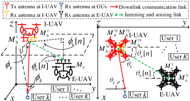
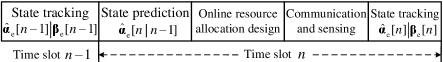
We consider a downlink UAV communication system where a hovering I-UAV¹¹1Mobile I-UAVs can further enhance PLS and will be considered in our future work. serves as a base station broadcasting $K$ independent confidential data streams to $K$ legitimate single-antenna GUs in the presence of a flying E-UAV, cf. Fig. 1. The I-UAV is equipped with two uniform planar arrays (UPAs) for 3-dimensional (3D) transmit (Tx) and receive (Rx) beamforming, respectively, comprising $M^{\mathrm{t}}_{\rm{b}}$ ($M^{\mathrm{tx}}_{\rm{b}}$ rows and $M^{\mathrm{ty}}_{\rm{b}}$ columns) and $M^{\mathrm{r}}_{\rm{b}}$ ($M^{\mathrm{rx}}_{\rm{b}}$ rows and $M^{\mathrm{ry}}_{\rm{b}}$ columns) antennas, respectively. The E-UAV is equipped with a Rx UPA, comprising $M_{\rm{e}}$ ($M^{\rm{x}}_{\rm{e}}$ rows and $M^{\rm{y}}_{\rm{e}}$ columns) antennas. The total service time $T$ is divided into $N$ equal-length time slots with a slot duration of $\delta$, i.e., $T=N\delta$. The locations of the I-UAV and GUs are denoted as $\mathbf{q}_{\mathrm{b}}=\left[x_{\mathrm{b}},y_{\mathrm{b}},z_{\mathrm{b}}\right]^{\mathrm{T}}$ and $\mathbf{q}_{k}=\left[x_{k},y_{k},0\right]^{\mathrm{T}}$, $\forall k$, respectively, where $[\cdot]^{\mathrm{T}}$ is the transpose operation. The E-UAV flies along a given trajectory, $\mathbf{q}_{\mathrm{e}}[n]=\left[x_{\mathrm{e}}[n],y_{\mathrm{e}}[n],z_{\mathrm{e}}[n]\right]^{\mathrm{T}}$, designed for intercepting the legitimate information transmission with velocity $\dot{\mathbf{q}}_{\mathrm{e}}[n]=[\dot{x}_{\mathrm{e}}[n],\dot{y}_{\mathrm{e}}[n],\dot{z}_{\mathrm{e}}[n]]^{\mathrm{T}}$, $n=\left\{1,\ldots,N\right\}$. The state of the E-UAV, $\bm{\alpha}_{\mathrm{e}}[n]=[\mathbf{q}^{\mathrm{T}}_{\mathrm{e}}[n],\dot{\mathbf{q}}^{\mathrm{T}}_{\mathrm{e}}[n]]^{\mathrm{T}}$, is unknown to the I-UAV. In contrast, the locations of both the I-UAV and GUs are known to the E-UAV. The time slot structure of the proposed ISJC scheme is illustrated in Fig. 2, where $\bm{\beta}_{\mathrm{e}}[n]$ represents all observable parameters at E-UAV. At the beginning of time slot $n$, I-UAV first predicts the state of E-UAV based on the state estimates in time slot $n-1$, i.e., $\hat{\bm{\alpha}}_{\mathrm{e}}[n|n-1]$. Based on the predicted state, I-UAV designs the resource allocation policy for time slot $n$ and broadcasts the information and the AN accordingly. Exploiting the echoes from E-UAV, I-UAV takes the new measurement $\bm{\beta}_{\mathrm{e}}[n]$ and estimates the new state of E-UAV $\hat{\bm{\alpha}}_{\mathrm{e}}[n]$, which is used as the input of the predictor for time slot $n+1$. Note that the considered system is inherently causal, where the resource allocation design in time slot $n$ is based on new measurements and new state estimates in time slot $n-1$.

The received signal at GU $k$ in time slot $n$ is given by

As the precoding policy of I-UAV is unknown to E-UAV, we assume that E-UAV performs maximum ratio combining (MRC) to maximize its received signal power. Assuming the azimuth and elevation angles-of-arrival (AoAs) are perfectly known at the E-UAV, the post-processed signal at E-UAV in time slot $n$ is

Based on (2), the achievable data rate of GU $k$ is given by

When E-UAV intercepts the information of GU $k$, as a worst case, we assume it can mitigate the inter-user interference of the other GUs and is only impaired by the AN. Thus, the leakage information rate associated with GU $k$ in time slot $n$ is given by

In practice, the signal transmitted by I-UAV is partially received by the Rx antennas of E-UAV and is partially reflected by its body. The I-UAV is assumed to operate in the full-duplex mode, which allows it to transmit and receive signals simultaneously, while the received signal may suffer residual self-interference[13]. The corresponding echo received at I-UAV in time slot $n$ is given by

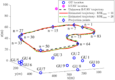
In this section, we evaluate the performance of the proposed ISJC scheme via simulations. The main simulation parameters are as follows: $K=10$, $\delta=1$ s, $N=92$, $p_{\mathrm{max}}=30$ dBm, ${R_{\mathrm{min}}}=5$ bit/s/Hz, ${R_{\mathrm{Leakage}}}=0.01$ bit/s/Hz, $G_{\mathrm{MF}}=10^{4}$, $\sigma^{2}_{\rm{e}}=\sigma^{2}_{k}=-99$ dBm, $\sigma^{2}_{\rm{b}}=-50$ dBm, $\beta^{2}_{0}=50$ dB, $\vartheta_{\mathrm{e}}=0.1$ $\rm m^{2}$, and ${M^{\mathrm{tx}}_{\mathrm{b}}}={M^{\mathrm{ty}}_{\mathrm{b}}}={M^{\mathrm{rx}}_{\mathrm{b}}}={M^{\mathrm{ry}}_{\mathrm{b}}}={M^{\mathrm{rx}}_{\mathrm{e}}}={M^{\mathrm{ry}}_{\mathrm{e}}}=4$. Note that a higher $\mathrm{MSE}_{\mathrm{max}}$ implies that a poorer tracking performance is tolerable by the considered system. Thus, we consider $\mathrm{MSE}_{\mathrm{max}}\in\left[5,26\right]$. The locations of I-UAV and the $K$ GUs and the unknown trajectory of E-UAV are illustrated in Fig. 3. The modeling parameters, including $c_{{\tau_{\rm{e}}}}$, $c_{\nu_{\rm{e}}}$, $c_{\theta_{\mathrm{be}}}$, $c_{\phi_{\mathrm{be}}}$, and $\mathbf{Q}_{\bm{\alpha}_{\mathrm{e}}}$, are initialized numerically assuming random walks of the I-UAV and E-UAV, respectively.

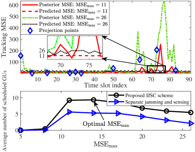
The estimated trajectory of E-UAV is shown in Fig. 3. The corresponding posterior tracking MSE, $\left\|\hat{{\bm{\alpha}}}_{\mathrm{e}}[n]-{{\bm{\alpha}}}_{\mathrm{e}}[n]\right\|^{2}$, in each time slot is shown in the upper half of Fig. 4. We observe that a smaller $\mathrm{MSE}_{\mathrm{max}}$ leads to a lower tracking MSE and a more accurate trajectory estimation. In fact, a smaller $\mathrm{MSE}_{\mathrm{max}}$ imposes a more stringent tracking MSE constraint for resource allocation design and thus more power and spatial degrees of freedom are allocated for sensing. To provide more insights, we define $K$ “projection points” on the unknown trajectory for which E-UAV has the smallest 3D distance w.r.t. the GUs, respectively. Comparing Fig. 3 and Fig. 4, we observe a high tracking MSE around some projection points, such as $n=64$ and $n=73$, where E-UAV changes directions, since the constant velocity model assumption for the EKF is less accurate in those points. Note that in Fig. 4, the posterior tracking MSE in some time slots is higher than $\mathrm{MSE}_{\mathrm{max}}$ while the predicted MSE is guaranteed to be smaller than $\mathrm{MSE}_{\mathrm{max}}$. In fact, $\mathrm{MSE}_{\mathrm{max}}$ only limits the predicted tracking MSE for resource allocation design while the actual tracking MSE, which is not accessible to the I-UAV at the time of resource allocation design, might be much higher due to the state evolution model mismatch and the measurement uncertainty in (10). Furthermore, the average number of scheduled GUs versus $\mathrm{MSE}_{\mathrm{max}}$ is shown in the lower half of Fig. 4. The performance of a baseline separate jamming and sensing scheme, where a dedicated sub-slot is used for sensing and the remaining time is used for communications and jamming, is also illustrated for comparison. We can observe a higher number of scheduled GUs for the proposed scheme compared to the benchmark scheme. This is because the dual use of AN in the proposed scheme preserves the system resources and provides more flexibility for resource allocation design. This underlines the advantage of integrating sensing, jamming, and communications for improving secrecy performance. It can be further observed that both a small $\mathrm{MSE}_{\mathrm{max}}$ and a large $\mathrm{MSE}_{\mathrm{max}}$ result in a small number of securely served GUs for both schemes. For a small $\mathrm{MSE}_{\mathrm{max}}$, more resources are needed for sensing, and thus, fewer GUs can be scheduled. This implies that enhancing the tracking performance is not always beneficial for communications as it requires more system resources. Increasing $\mathrm{MSE}_{\mathrm{max}}$ relaxes the tracking performance constraint C4 in (18) and thus results in a larger objective value. However, a too large $\mathrm{MSE}_{\mathrm{max}}$ in a given time slot leads to unreliable eavesdropper channel prediction in the next time slot, and thus, a lower jamming efficiency. Hence, the number of securely served GUs is ultimately limited by the channel prediction uncertainty in the large $\mathrm{MSE}_{\mathrm{max}}$ regime. In fact, choosing $\mathrm{MSE}_{\mathrm{max}}$ properly is critical for maximizing the secrecy communication performance. For example, for the considered scenario, $\mathrm{MSE}_{\mathrm{max}}=14$ is optimal for the proposed scheme.

In this paper, we proposed a novel ISJC framework and an online resource allocation design for securing UAV-enabled downlink communications. The dual use of AN enables the I-UAV to concurrently jam the E-UAV and sense the corresponding channels efficiently. Through simulations, we demonstrated that integrating sensing, jamming, and communications improves the secrecy performance, while choosing a suitable value for the tolerable tracking MSE is critical for balancing tracking and secrecy performance.

References

- [1] Qingqing Wu, Jie Xu, Yong Zeng, Derrick Wing Kwan Ng, Naofal Al-Dhahir, Robert Schober, and A. Lee Swindlehurst, “A comprehensive overview on 5G-and-Beyond networks with UAVs: From communications to sensing and intelligence,” IEEE J. Select. Areas Commun., vol. 39, no. 10, pp. 2912–2945, Oct. 2021.
- [2] Zhiqiang Wei, Yuanxin Cai, Zhuo Sun, Derrick Wing Kwan Ng, Jinhong Yuan, Mingyu Zhou, and Lixin Sun, “Sum-rate maximization for IRS-assisted UAV OFDMA communication systems,” IEEE Trans. Wireless Commun., vol. 20, no. 4, pp. 2530–2550, Apr. 2021.
- [3] Qingqing Wu, Weidong Mei, and Rui Zhang, “Safeguarding wireless network with UAVs: A physical layer security perspective,” IEEE Wireless Commun., vol. 26, no. 5, pp. 12–18, Oct. 2019.
- [4] Qian Wang, Zhi Chen, Weidong Mei, and Jun Fang, “Improving physical layer security using UAV-enabled mobile relaying,” IEEE Wireless Commun. Lett., vol. 6, no. 3, pp. 310–313, Jun. 2017.
- [5] Guangchi Zhang, Qingqing Wu, Miao Cui, and Rui Zhang, “Securing UAV communications via joint trajectory and power control,” IEEE Trans. Wireless Commun., vol. 18, no. 2, pp. 1376–1389, Feb. 2019.
- [6] Xiaobo Zhou, Qingqing Wu, Shihao Yan, Feng Shu, and Jun Li, “UAV-enabled secure communications: Joint trajectory and transmit power optimization,” IEEE Trans. Veh. Technol., vol. 68, no. 4, pp. 4069–4073, Apr. 2019.
- [7] Yuanxin Cai, Zhiqiang Wei, Ruide Li, Derrick Wing Kwan Ng, and Jinhong Yuan, “Joint trajectory and resource allocation design for energy-efficient secure UAV communication systems,” IEEE Trans. Commun., vol. 68, no. 7, pp. 4536–4553, Jul. 2020.
- [8] Miao Cui, Guangchi Zhang, Qingqing Wu, and Derrick Wing Kwan Ng, “Robust trajectory and transmit power design for secure UAV communications,” IEEE Trans. Veh. Technol., vol. 67, no. 9, pp. 9042–9046, Sep. 2018.
- [9] Zhongxiang Wei, Fan Liu, Christos Masouros, Nanchi Su, and Athina P Petropulu, “Towards multi-functional 6G wireless networks: Integrating sensing, communication and security,” arXiv preprint arXiv:2107.07735, 2021.
- [10] Nanchi Su, Fan Liu, Zhongxiang Wei, Ya-Feng Liu, and Christos Masouros, “Secure dual-functional radar-communication transmission: Exploiting interference for resilience against target eavesdropping,” arXiv preprint arXiv:2107.04747, 2021.
- [11] Nanchi Su, Fan Liu, and Christos Masouros, “Secure radar-communication systems with malicious targets: Integrating radar, communications and jamming functionalities,” IEEE Trans. Wireless Commun., vol. 20, no. 1, pp. 83–95, 2021.
- [12] Harry L Van Trees, Optimum Array Processing: Part IV of Detection, Estimation and Modulation Theory, John Wiley & Sons, 2004.
- [13] Yan Sun, Derrick Wing Kwan Ng, Jun Zhu, and Robert Schober, “Robust and secure resource allocation for full-duplex MISO multicarrier NOMA systems,” IEEE Trans. Commun., vol. 66, no. 9, pp. 4119–4137, Sep. 2018.
- [14] Merrill I Skolnik, Introduction to Radar, McGraw-hill New York, NY, USA, 1962.
- [15] Fan Liu, Weijie Yuan, Christos Masouros, and Jinhong Yuan, “Radar-assisted predictive beamforming for vehicular links: Communication served by sensing,” IEEE Trans. Wireless Commun., vol. 19, no. 11, pp. 7704–7719, Nov. 2020.
- [16] Steven M Kay, Fundamentals of Statistical Signal Processing: Estimation Theory, Prentice-Hall, Inc., 1993.
- [17] Brian DO Anderson and John B Moore, Optimal Filtering, Courier Corporation, 2012.
- [18] George Fishman, Monte Carlo: Concepts, Algorithms, and Applications, Springer Science & Business Media, 2013.
- [19] Zhiqiang Wei, Derrick Wing Kwan Ng, Jinhong Yuan, and Hui-Ming Wang, “Optimal resource allocation for power-efficient MC-NOMA with imperfect channel state information,” IEEE Trans. Commun., vol. 65, no. 9, pp. 3944–3961, Sep. 2017.
- [20] S Boyd and L Vandenberghe, Convex Optimization, Cambridge University Press, 2004.
- [21] Zhi-Quan Luo, Wing-Kin Ma, Anthony Man-Cho So, Yinyu Ye, and Shuzhong Zhang, “Semidefinite relaxation of quadratic optimization problems,” IEEE Signal Process. Mag., vol. 27, no. 3, pp. 20–34, May 2010.