Safe-FinRL: A Low Bias and Variance Deep Reinforcement Learning Implementation for High-Freq Stock Trading

Generally, DRL algorithms can be categorized into three approaches: value-based algorithm, policy-based algorithm, and actor-critic algorithm. For value-based algorithms, they mainly focus on the discrete action space control problem and use the bellman equation to update. Among them, Deep Q-Network (DQN) (Mnih et al., 2015, 2013) adapts Q-learning and eplison-greedy technique, and it has been successfully applied to playing video games. For policy-based algorithm, Proximal Policy Optimization (PPO) (Schulman et al., 2017) and Trust Region Policy Optimization (TRPO) (Schulman et al., 2015a) improve the vanilla Policy Gradient (Sutton et al., 1999) by introducing Importance Sampling (IS) to correct the distribution shift and Generalized Advantage Estimation (GAE) (Schulman et al., 2015b) to obtain stable and steady improvement in some 3D-locomotion tasks. For actor-critic based algorithm, Deep Deterministic Policy Gradient (DDPG) (Lillicrap et al., 2015) and Twin-Delayed DDPG (TD3) (Fujimoto et al., 2018) uses value and policy function as two function approximators and optimize them simultaneously. Soft Actor-Critic (SAC) (Haarnoja et al., 2018) introduces an additional entropy term to its objective function to facilitate exploration based on DDPG and TD3.

In many real-world DRL applications, interaction with the environment is costly, and we want to reuse the sample trajectories collected before. This necessitates the use of off-policy DRL methods, algorithms that can learn from previous experience collected by possibly unknown behavior policies. In the actor-critic algorithm, its value function is learned by iteratively solving the Bellman Equation, which is inherently off-policy and independent of any underlying data distribution (Nachum et al., 2019b). Nevertheless, when multi-step returns are used to control bias in off-policy learning, the distribution shift between target policy and behavior policy will occur inevitably. Importantly, this discrepancy can lead to complex, non-convergent behavior of value function in the algorithm (Kozuno et al., 2021).

Currently, there are two main approaches two handle this distribution shift. One approach is to manually correct the shift by setting ‘trace values’ to the multi-step bellman equations. Among them, Retrace (Munos et al., 2016), Tree-Backup (TBL) (Precup, 2000) are conservative methods that the convergence of value function is guaranteed no matter what behavior policy is used. By contrast, C-trace (Rowland et al., 2020), Peng’s Q($\lambda$) (PQL) (Peng, Williams, 1994), and uncorrected n-step return are non-conservative methods that do not damp the trace value or truncate trajectories, and thus do not guarantee generic convergence. Importantly, the ‘trace’ approach can be extended to the actor-critic settings easily. Another approach, DItribution Correction Estimation (DICE) families (Nachum et al., 2019b, a), are alternatives to the policy gradient and value-based methods, which directly give the estimation of the distribution shift by introducing a new formulation of max-return optimization.

Among the recent research on DRL applications for stock trading, many of them follow the model-free off-policy DRL settings. Jiang et al. (2017) apply Deterministic Policy Gradient (DPG) to the portfolio allocation problem of cryptocurrency. Liang et al. (2018) model stock trading as a continuous control problem and implement DDPG and PPO for portfolio management in China’s stock market. Liu et al. (2020) introduce a DRL library called FinRL and implement several benchmarking DRL algorithms to construct profitable trading strategies in S&P 500 index. Wang et al. (2021) develop a hierarchy DRL that contains a high-level RL to control the portfolio weights and a low-level RL to decide the specific selling price and quantities. Fang et al. (2021) implement an RL Oracle by distilling actions from future stock information. Despite many of them claiming to be profitable, very few of them have customized their DRL models to the heterogeneous and volatile financial environment.

Under the assumption that the pricing of one financial asset only depends on its previous prices within a certain range, we model the stock trading process as a Markovian Process. Specifically, when trading an asset in the real financial market, both the price and the decision of selling or buying the asset at time step $t$ are singly determined by their previous information, and the return of that decision is singly generated by the price changing from time $t$ to $t+1$. Consequently, the financial task of trading assets can be modeled as a Markov Decision Process (MDP). The detailed definitions of the state space, action space, and reward function in our model are shown below.

State Space $\mathcal{S}$. Normally, state space of financial assets only contain their previous pricing information $\mathbf{p_{t}}$. In our work, we extend the state space $\mathbf{s_{t}}$ in three direction. First, we add over 118 technical features $\mathbf{q_{t}}$ for each asset in the high-frequency trading market at time $t$ to the original pricing information. Second, we incorporate the remaining balance $\mathbf{b_{t}}$ and holding shares for each asset $\mathbf{h_{t}}$ as a part of state space at time $t$. Finally, instead of looking at single time $t$’s information, we use a look-back window with length $l$ (default:3) and enlarge $\mathbf{s_{t}}$ by stacking previous information from $t-l$ to $t$. In summary, $\mathbf{s_{t}}$ contains three parts,

• •

  Balance $\mathbf{b_{t}}$: the amount of money left in the account at the time step $t$

• •

  Holding Shares $\mathbf{s_{t}}$: the amount of holding shares for each asset at time step $t$.

• •

  Features $\{\mathbf{q_{t-l:t}},\mathbf{p_{t-l:t}}\}$: technical and price features for each asset from time step $t-l$ to $t$.

Action Space $\mathcal{A}$. The action space of trading one asset is formulated by a continuous one-dimension vector $\mathbf{a_{t}}\in[-h\_max,h\_max]$ that represents the confidence of longing or shorting that asset, where $h\_max$ is the upper and lower bound of the action (default:0.1). When $\mathbf{a_{t}}$ closes to $h\_max$, it represents a strong signal to buy that asset. On the contrary, $\mathbf{a_{t}}$ closes to $-h\_max$ represents high confidence to sell that asset. The amount of selling or buying shares are calculated by $\lfloor\frac{\mathbf{a_{t}}}{u}\rfloor\cdot u$, where $u$ is the minimum trading unit in the high frequency trading market.

Reward $\mathcal{R}(s,a,s^{\prime})$. Consider $s^{\prime}$ is the new arriving state when action $a$ is taken at state $s$. Reward $r(s,a,s^{\prime})$ is formulated by $\log(\frac{v^{\prime}}{v})$, where $v^{\prime}$ and $v$ is the total amount of wealth at state $s^{\prime}$ and state $s$. Specifically, at time t, $v_{t}=b_{t}+p_{t}\cdot a_{t}\cdot\text{sgn}(-a_{t})\cdot(1+\text{sgn}(a_{t})\cdot c)$, where $c$ is the commission fee and $p_{t}$ is the sell/bid price when $a_{t}<0$ and $p_{t}$ is the buy/ask price when $a_{t}>0$.

Since in the financial market, the transition probability from state $s_{t}$ to state $s_{t+1}$ can not be explicitly modeled, based on OpenAI Gym, we build an artificial trading environment with real-life market data. Unlike trading in the real world, we have loosened restrictions on positions, assuming that the agent can buy and sell any amount of shares in that trading environment. Finally, the trading robot can observe states, take actions of long and short, receive rewards, and have its strategy adjusted accordingly through iteratively interacting with the built artificial trading environment.

The raw data of the real life market consists of snapshots of order book data and tick-by-tick trade data of the btc-usdt swap of Binance. We aggregate the raw data by minute and formulate 118 meaningful predictors as features. All features are standardized by z-score to ensure the stability of the model. We also designed a trade book that contains bid prices and ask prices at the end of each minute for simulated trading since the spread is crucial in high-frequency trading. The data is for 20 days, from March 10, 2022 to March 29, 2022. After processing, the total sample size is around 28800.

In this work, we choose the single-step Soft Actor-Critic (SAC) (Haarnoja et al., 2018) as our benchmark algorithm. This is because through generating a stochastic policy and maximizing an adjustable entropy term in its objective function, SAC can capture multiple modes of near-optimal behavior and thus has superior exploration ability over other deterministic policy algorithms such us DDPG (Lillicrap et al., 2015) and TD3 (Fujimoto et al., 2018). In our experiment, we find that setting the weight of the entropy term in SAC to be constant will help convergence, so we choose to use SAC with an unadjustable entropy term as the benchmark. Moreover, we also use the market value itself as one of our benchmarks.

Here, we separate the twenty days of trading data into four independent near-stationary environments to reduce the negative effect of a non-stationary stock trading environment. Each separated environment contains five days of trading data, of which three days are used to train, and the left two days are used to do validation and test. In Figure 1, we present the detailed process. From the figure, we can observe that the consecutive four environments indeed are highly heterogeneous. In Env₀, the stock price displays an obvious descending trend while Env₃ witnesses a remarkable stock price spike. On the contrary, the stock price trend within each environment is more stable and predictable than the highly non-stationary trend between separated environments.

We first briefly review the definitions of policy and value functions in RL and build up the necessary knowledge for multi-step TD learning. Next, we introduce the off-policy multi-step TD learning based on the General Retrace operator (Munos et al., 2016). Finally, we explain the proposed Trace-SAC algorithms.

Single-Step Estimation. We consider the standard off-policy RL setup where an agent interacts with an environment, generating a sequence of state-action-reward-state tuples $(s_{t},a_{t},r_{t},s_{t+1})$, where $s_{t},s_{t+1}\in\mathcal{S}$ and $a_{t}\in\mathcal{A}$ which is sampled from some policy $\pi_{k}:\mathcal{S}\to[0,1]$. Here we define the discounted cumulative return start at time $t$ as $G_{t}:=\sum_{t^{\prime}=t}^{\infty}\gamma^{t^{\prime}-t}r_{t^{\prime}}$. The value function and Q-function at time $t$ are defined by $V^{\pi_{k}}(s_{t}):=\mathbb{E}_{\pi_{k}}[G_{t}|s_{t}]$ and $Q^{\pi_{k}}(s_{t},a_{t}):=\mathbb{E}_{\pi_{k}}[G_{t}|s_{t},a_{t}]$, respectively, where the expectation over $\pi_{k}$ means $a_{t}\sim\pi_{k}(\cdot|s_{t})$.

Since large continuous domains require us to design practical function approximators for both policy and value function, we assume Q-function $Q_{\theta}:\mathcal{S}\times\mathcal{A}\to\mathbb{R}$ is parameterized by $\theta$ and policy function $f_{\phi}:\mathcal{S}\to\mathcal{A}$ is parameterized by $\phi$. Based on that, the single step bellman operator $Q_{k+1}:=\mathcal{B}^{\pi_{k}}Q_{k}$ and bellman optimal operator $Q_{k+1}^{*}:=\mathcal{B}^{*}Q_{k}^{*}$ are given by:

where $\rho_{\pi_{k}}(s_{t})$ is the state marginal of the trajectory distribution induced by policy $\pi_{k}$. Next, the Temporal Difference (TD) or single-step bellman error is obtained by $\delta_{t}:=\mathcal{B}^{\pi_{k}}Q_{k}(s_{t},a_{t})-Q_{k}(s_{t},a_{t})$ and $\delta_{t}^{*}:=\mathcal{B}^{*}Q_{k}(s_{t},a_{t})-Q_{k}(s_{t},a_{t})$. Importantly, the first obtained $\delta_{t}$ is often used in the value function approximation in some actor-critic algorithms, such us DDPG (Lillicrap et al., 2015) while the second $\delta_{t}^{*}$ is used in the standard Q-learning algorithm (Watkins, Dayan, 1992). Finally, by using Stochastic Approximation (Robbins, Monro, 1951), we approximate the Q-function by iteratively calculating:

where $\alpha_{k}\to 0$ as $k\to\infty$.

General Retrace. Munos et al. (2016) extend the single-step value function estimation in (4) and introduce a general retrace operator to estimate the value function using both off-policy and multi-step TD learning, from which the distribution correction can be obtained by singly changing the trace value. Specifically, the general retrace algorithm updates its Q-function by $Q_{k+1}:=\mathcal{R}_{\lambda}^{c_{k},\mu_{k},\pi_{k}}Q_{k}$, where $(c_{k})_{k\geq 0}$ is a sequence of non-negative functions over $\mathcal{S}\times\mathcal{A}$. $(\mu_{k})_{k\geq 0}$ is an arbitrary sequence of behavior policies, and $(\pi_{k})_{k\geq 0}$ is a sequence of target policies that depends on an algorithm. Given a trajectory $(s_{t},a_{t},r_{t},s_{t+1})_{t\geq 0}$ collected under $\mu_{k}$, the general retrace algorithm $Q_{k+1}(s_{t},a_{t}):=(\mathcal{R}_{\lambda}^{c_{k},\mu_{k},\pi_{k}}Q_{k})(s_{t},a_{t})$ can be written as:

where $\prod_{u=1}^{t}c_{k}(s_{u},a_{u}):=1$ and $\delta_{t}=\mathcal{B}^{\mu_{k}}Q_{k}(s_{t},a_{t})-Q_{k}(s_{t},a_{t})$.

Trace-SAC. In the single-step Soft Actor Critic (Haarnoja et al., 2018), its target is adjusted to maximize a soft Q-function $Q^{soft}(s_{t},a_{t}):=r_{t}+\mathbb{E}_{(s_{t+1},\cdots)\sim\rho_{\pi}}[\sum_{l=1}^{\infty}\gamma^{l}(r_{t+l}+\alpha\mathcal{H}(\pi^{*}_{\text{MaxEnt}}(\cdot|s_{t+l})))]$, where $\mathcal{H}(\cdot)$ is the Shannon entropy and the details of $\pi^{*}_{\text{MaxEnt}}$ can be found in (Haarnoja et al., 2017). Based on that, the soft policy evaluation is defined as $Q_{k+1}^{soft}:=\mathcal{T^{\pi}}Q_{k}^{soft}$, where $Q^{soft}:\mathcal{S}\times\mathcal{A}\to\mathbb{R}$ and $\mathcal{T}^{\pi}$ is a modified bellman backup operator. Given a single step tuple $(s_{t},a_{t},r_{t},s_{t+1})$, the modified bellman backup operator is given by:

where $\rho_{\pi_{k}}(s_{t})$ is the state marginal of the trajectory distribution induced by policy $\pi_{t}$. According to Haarnoja et al. (2018), the soft bellman backup operator $\mathcal{T}^{\pi}$ shares a similar convergence property as $\mathcal{B}^{\pi}$. Specifically, the sequence $Q_{k}^{soft}$ will converge to the soft Q-value of policy $\pi$ as $k\to\infty$. This motivates us incorporate SAC into the General Retrace algorithm.

In the Trace-SAC we proposed, we use the convergence property of soft bellman backup operator $\mathcal{T}^{\pi}$ and integrate SAC into the General Retrace algorithm. In practice, the Trace-SAC updates its Q-function by $Q_{k+1}^{soft}:=\mathcal{R^{\prime}}_{\lambda}^{c_{k},\mu_{k},\pi_{k}}Q_{k}^{soft}$, where $(c_{k})_{k\geq 0}$ is a sequence of non-negative functions over $\mathcal{S}\times\mathcal{A}$. $(\mu_{k})_{k\geq 0}$ is an arbitrary sequence of behavior policies, and $(\pi_{k})_{k\geq 0}$ is a sequence of target policies that depends on an algorithm. Given a trajectory $(s_{t},a_{t},r_{t},s_{t+1})_{t\geq 0}$ collected under $\mu_{k}$, the soft value function estimation for Trace-SAC can be written as:

where $\prod_{u=1}^{t}c_{k}(s_{u},a_{u}):=1$ and $\delta_{t^{\prime}}=\mathcal{T}^{\mu_{k}}Q_{k}^{soft}(s_{t^{\prime}},a_{t^{\prime}})-Q_{k}^{soft}(s_{t^{\prime}},a_{t^{\prime}})$. Importantly, when $T,\lambda,c_{k}=0$, it returns to the single-step SAC.

Given the choices of $c_{k}$ and $\pi_{k}$ in Table 1, we recover a few known algorithms (Peng, Williams, 1994; Precup, 2000; Munos et al., 2016). Importantly, according to (Kozuno et al., 2021), an algorithm is called conservative, if $c_{k}(s,a)\in[0,\pi_{k}(a|s)/\mu_{k}(a|s)]$ for any $k$ and $(s,a)\in\mathcal{S}\times\mathcal{A}$. See Table 1 for the classification of algorithms. Through choosing different trace algorithms (conservative or non-conservative) and controlling the values of $T$ and $\lambda$ in Equation (7), Trace-SAC is able to handle the trade-off of bias and variance in the off-policy value estimation in the financial environment.

Parameter Updates. As discussed above, large continuous action space drive us to use function approximators for both the Q-function and policy function. To that end, we consider parameterized soft Q-function $Q_{\theta}(s_{t},a_{t})$, a tractable policy distribution $\pi_{\phi}(\cdot|s_{t})\in[0,1]$, and a policy function $a_{t}=f_{\phi}(s_{t};\epsilon)$, where $f_{\phi}$ is realized by the reparameterization trick using a network transformation. The parameters of these neural networks are $\theta$ and $\phi$ respectively. In practice, we use the Long Short Term Network (LSTM) (Hochreiter, Schmidhuber, 1997) to encoder the stock features for both value and policy approximators. The value function is followed by Fully Connected Layers to output a single Q-value while the policy output mean and standard deviation vectors to parameterize Gaussian distribution with the support in [-h_max,h_max]. We will next dive into the update rules for these parameter vectors.

The update rules for Trace-SAC is very similar to the original SAC algorithm. Suppose $\mathcal{D}$ is the replay buffer, the multi-step soft value function is trained to minimize the Least Square Temporal Difference (LSTD):

where $\mathcal{R^{\prime}}_{\lambda}^{c_{k},\mu_{\phi_{k}},\pi_{\phi_{k}}}$is the Trace-SAC operator discussed above. Next, the policy parameters can be learned by minimizing:

Since we disable the self-tuning for the alpha in the original SAC and set it to be a constant term, there is no loss for the alpha function. Finally, putting Equation (8) and (9) together, the update of $\theta$ and $\alpha$ are given by $\theta_{k+1}\leftarrow\theta_{k}-\lambda_{\theta}\nabla_{\theta}L_{Q}(\theta_{k})$ and $\phi_{k+1}\to\phi_{k}-\lambda_{\phi}\nabla_{\phi}L_{\pi}(\phi)$.

Furthermore, Trace-SAC also exploits the double Q-learning structure to mitigate positive bias in the policy improvement step which is known to deteriorate the performance of estimating value function (Hasselt, 2010). Generally, Trace-SAC alternates between collecting experience from the financial environment with the current policy and updating the function approximators using behavior policies sampled from a replay buffer. In practice, we allow the Trace-SAC agent to take a single environment step followed by several gradient steps so that it can better capture the patterns in the financial environment. We also observe that using delayed policy updates in the financial environment will also facilitate the convergence of value function.

We evaluate the overall performance of the proposed Trace-SAC on the four independent environments shown in Figure 1. On each separated environment, we use the cumulative log return $R_{t}$ from start time $t$ to end time $T$ on the validation set as the performance metric. Mathematically, it is given by $R_{t}=\log(v_{T}/v_{0})$, where $v_{T}$ is the total wealth at the termination state and $v_{0}$ is the initial wealth or balance the trading agent holds. Furthermore, our experiment uses the market value and single-step SAC as two benchmarks.

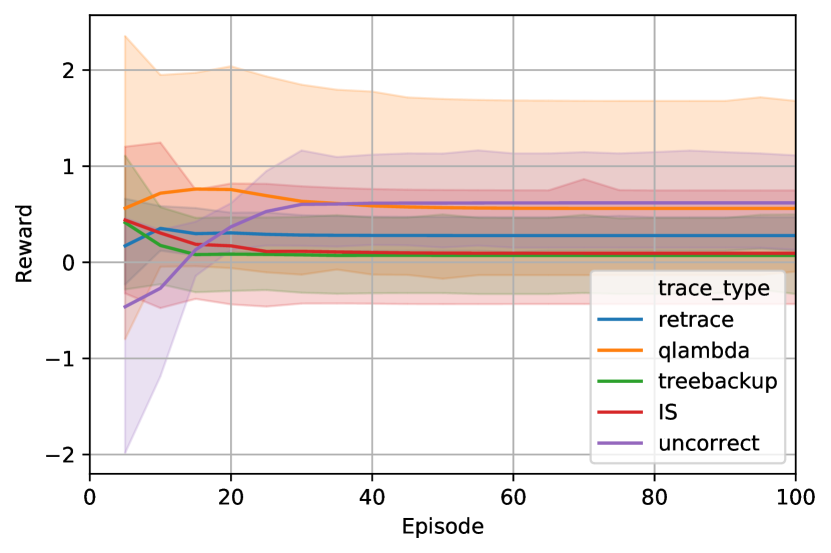
In Table 2, we conduct the experiment on five different Trace-SAC algorithms in the four environments. Specifically, we choose (1) Retrace; (2) Tree Backup; (3) Peng’s Q($\lambda$) with a fixed $\lambda$; (4) Importance Sampling; (5) Uncorrect n-step with a fixed n to compare with the baselines. Among all the multi-step algorithms, Importance Sampling is conservative and is often the most used algorithm to correct the distribution shift. Retrace is also a representative conservative, while the uncorrected n-step operator is the most commonly used non-conservative operator. The reward curves on the four environments, along with five different algorithms, are shown in Figure 2.

From Table 2, we can observe that the five trace algorithms implemented on SAC generally have higher rewards than the single-step SAC in all of the four environments. Interestingly, we discover the single-step SAC has a much higher variance than the multi-step algorithms, especially in Env1 and Env3. Moreover, we observe that the non-conservative algorithms like Q($\lambda$) and uncorrected TD($\lambda$) have remarkably outperformed the conservative ones like IS and Retrace in Env0 and Env1. This observation is consistent with the theoretical finding in Kozuno et al. (2021), which explains the reason non-conservative algorithms empirically outperform the conservative ones is that the convergence to the optimal policy is recovered when the behavior policy closely tracks the target policy.

In Figure 3, we train the Trace-SAC using a conservative Retrace algorithm and validate it on the four independent environments. We observe that Trace-SAC has a nice convergence property in all four financial environments. Meanwhile, combined with the information in Table 2, retrace gives a lower variance than the other four trace algorithms.

To see the training difference between the four environments, we observe that Trace-SAC has significantly outperformed the market in Env0, and it also has successfully overtaken the market after 40 episodes in Env2. However, retrace has severely underperformed the market in both Env1 and Env3. Combining with the individual environment information in Figure 1, we observe that in Env1, the training environment (red shaded area) is in an active accenting area while the validation environment (yellow and green shaded area) is either in a plateau or in a passive descending area. Similarly, in Env3, the training environment (red shaded area) is in a flat and smooth ascending period, while the validation environment displays a sudden jump from the basin. These discrepancies between the training and validation environment may cause the Trace-SAC agent to fail to capture the trends and underperform the market.

References

- Fang et al. (2021) Fang Yuchen, Ren Kan, Liu Weiqing, Zhou Dong, Zhang Weinan, Bian Jiang, Yu Yong, Liu Tie-Yan. Universal Trading for Order Execution with Oracle Policy Distillation // arXiv preprint arXiv:2103.10860. 2021.
- Fujimoto et al. (2018) Fujimoto Scott, Hoof Herke, Meger David. Addressing function approximation error in actor-critic methods // International conference on machine learning. 2018. 1587–1596.
- Haarnoja et al. (2017) Haarnoja Tuomas, Tang Haoran, Abbeel Pieter, Levine Sergey. Reinforcement learning with deep energy-based policies // International Conference on Machine Learning. 2017. 1352–1361.
- Haarnoja et al. (2018) Haarnoja Tuomas, Zhou Aurick, Abbeel Pieter, Levine Sergey. Soft actor-critic: Off-policy maximum entropy deep reinforcement learning with a stochastic actor // International conference on machine learning. 2018. 1861–1870.
- Hasselt (2010) Hasselt Hado. Double Q-learning // Advances in neural information processing systems. 2010. 23.
- Hochreiter, Schmidhuber (1997) Hochreiter Sepp, Schmidhuber Jürgen. Long short-term memory // Neural computation. 1997. 9, 8. 1735–1780.
- Jiang et al. (2017) Jiang Zhengyao, Xu Dixing, Liang Jinjun. A deep reinforcement learning framework for the financial portfolio management problem // arXiv preprint arXiv:1706.10059. 2017.
- Kozuno et al. (2021) Kozuno Tadashi, Tang Yunhao, Rowland Mark, Munos Rémi, Kapturowski Steven, Dabney Will, Valko Michal, Abel David. Revisiting Peng’s Q ( ) for Modern Reinforcement Learning // International Conference on Machine Learning. 2021. 5794–5804.
- Liang et al. (2018) Liang Zhipeng, Chen Hao, Zhu Junhao, Jiang Kangkang, Li Yanran. Adversarial deep reinforcement learning in portfolio management // arXiv preprint arXiv:1808.09940. 2018.
- Lillicrap et al. (2015) Lillicrap Timothy P, Hunt Jonathan J, Pritzel Alexander, Heess Nicolas, Erez Tom, Tassa Yuval, Silver David, Wierstra Daan. Continuous control with deep reinforcement learning // arXiv preprint arXiv:1509.02971. 2015.
- Liu et al. (2020) Liu Xiao-Yang, Yang Hongyang, Chen Qian, Zhang Runjia, Yang Liuqing, Xiao Bowen, Wang Christina Dan. Finrl: A deep reinforcement learning library for automated stock trading in quantitative finance // arXiv preprint arXiv:2011.09607. 2020.
- Mnih et al. (2013) Mnih Volodymyr, Kavukcuoglu Koray, Silver David, Graves Alex, Antonoglou Ioannis, Wierstra Daan, Riedmiller Martin. Playing atari with deep reinforcement learning // arXiv preprint arXiv:1312.5602. 2013.
- Mnih et al. (2015) Mnih Volodymyr, Kavukcuoglu Koray, Silver David, Rusu Andrei A, Veness Joel, Bellemare Marc G, Graves Alex, Riedmiller Martin, Fidjeland Andreas K, Ostrovski Georg, others . Human-level control through deep reinforcement learning // nature. 2015. 518, 7540. 529–533.
- Munos et al. (2016) Munos Rémi, Stepleton Tom, Harutyunyan Anna, Bellemare Marc. Safe and efficient off-policy reinforcement learning // Advances in neural information processing systems. 2016. 29.
- Nachum et al. (2019a) Nachum Ofir, Chow Yinlam, Dai Bo, Li Lihong. Dualdice: Behavior-agnostic estimation of discounted stationary distribution corrections // Advances in Neural Information Processing Systems. 2019a. 32.
- Nachum et al. (2019b) Nachum Ofir, Dai Bo, Kostrikov Ilya, Chow Yinlam, Li Lihong, Schuurmans Dale. Algaedice: Policy gradient from arbitrary experience // arXiv preprint arXiv:1912.02074. 2019b.
- Peng, Williams (1994) Peng Jing, Williams Ronald J. Incremental multi-step Q-learning // Machine Learning Proceedings 1994. 1994. 226–232.
- Precup (2000) Precup Doina. Eligibility traces for off-policy policy evaluation // Computer Science Department Faculty Publication Series. 2000. 80.
- Robbins, Monro (1951) Robbins Herbert, Monro Sutton. A stochastic approximation method // The annals of mathematical statistics. 1951. 400–407.
- Rowland et al. (2020) Rowland Mark, Dabney Will, Munos Rémi. Adaptive trade-offs in off-policy learning // International Conference on Artificial Intelligence and Statistics. 2020. 34–44.
- Schulman et al. (2015a) Schulman John, Levine Sergey, Abbeel Pieter, Jordan Michael, Moritz Philipp. Trust region policy optimization // International conference on machine learning. 2015a. 1889–1897.
- Schulman et al. (2015b) Schulman John, Moritz Philipp, Levine Sergey, Jordan Michael, Abbeel Pieter. High-dimensional continuous control using generalized advantage estimation // arXiv preprint arXiv:1506.02438. 2015b.
- Schulman et al. (2017) Schulman John, Wolski Filip, Dhariwal Prafulla, Radford Alec, Klimov Oleg. Proximal policy optimization algorithms // arXiv preprint arXiv:1707.06347. 2017.
- Sutton et al. (1999) Sutton Richard S, McAllester David, Singh Satinder, Mansour Yishay. Policy gradient methods for reinforcement learning with function approximation // Advances in neural information processing systems. 1999. 12.
- Wang et al. (2021) Wang Rundong, Wei Hongxin, An Bo, Feng Zhouyan, Yao Jun. Deep Stock Trading: A Hierarchical Reinforcement Learning Framework for Portfolio Optimization and Order Execution // arXiv preprint arXiv:2012.12620. 2021.
- Watkins, Dayan (1992) Watkins Christopher JCH, Dayan Peter. Q-learning // Machine learning. 1992. 8, 3. 279–292.