Safe and Stable Formation Control with Distributed Multi-Agents Using Adaptive Control and Control Barrier Functions
Abstract
This manuscript considers the problem of ensuring stability and safety during formation control with distributed multi-agent systems in the presence of parametric uncertainty in the dynamics and limited communication. We propose an integrative approach that combines Control Barrier Functions, Adaptive Control, and connected graphs. A reference model is designed so as to ensure a safe and stable formation control strategy. This is combined with a provably correct adaptive control design that includes the use of a CBF-based safety filter that suitably generates safe reference commands. Numerical examples are provided to support the theoretical derivations.
I Introduction
Multi-agent systems (MAS) have received much attention because of their potential in completing tasks that a single agent could not complete efficiently on their own. Examples include exploration, surveillance, reconnaissance, rescue, and failure-tolerance, which occur in various problems related to motion planning and robotics. Typical problems in the context of MAS include consensus, formation control, coordination, and synchronization. This paper pertains to formation control.
The concept of formation control can be classified into the formation tracking and formation producing. In the former, the agents maintain a desired trajectory while the configuration itself moves through space; this is of interest for problems related to rendezvous in air and space. In the latter, the objective is to converge to a static formation from some initial configuration of the agents, which is useful in tasks of surveillance and more generally sensor deployment. Our paper focuses on the latter. We will focus on a class of dynamic MAS which are subjected to parametric uncertainties, state-space constraints, and limited communication among the agents, and the goal is to achieve a real-time control solution that accomplishes a static formation task.
Several approaches have been reported in the literature to achieve formation control, but with a subset of the above features. The approaches in [1], [2], and [3] have addressed the formation control problem in the presence of parametric uncertainty using adaptive control. No constraints on the state or in the communication among agents are however considered. The solutions in [4], [5], and [6] focus on formation control with limited communication and parametric uncertainties, but do not address obstacles or other state-space constraints. The authors of [7, 8, 9, 10, 11, 12, 13] consider obstacles and formation control with limited communication, but assume full knowledge of the agent dynamics. The authors of [14] and [15] consider obstacles and parametric uncertainty but assume full communication between all agents.
In contrast to the above papers, the authors of [16, 17, 18] have addressed, as in this paper, formation control for distributed MAS amidst obstacles and parametric uncertainties. However the following distinctions can be made: The results in [16] limit the uncertainty to a constant additive disturbance that is unknown. The solutions in [17] and [18] consider general nonlinear dynamics that is unknown, and employ a neural-network based solution. In this paper, we propose an adaptive control solution for static formation control in the presence of parametric uncertainties, obstacles which introduce safety considerations, and limited communication among agents. The unique features of our proposed solution are (i) the use of a Graph Control Barrier Function that shapes the reference input so as to ensure safety, (ii) the use of a reference model that leverages the communication structure among the distributed MAS, and (iii) an analytically rigorous stability proof that guarantees boundedness of all signals and convergence to the desired formation.
Preliminaries are presented in Section II and the control problem in Section III. The main contribution of this manuscript, the development of an adaptive controller with stability and safety properties, is presented in Section IV. Section V includes numerical simulations. Proofs of the main contributions of the manuscript (Theorems 2 and 3) are presented in the appendix.
II Preliminaries
II-A Graph Theory and Multi-Agent Systems Communication
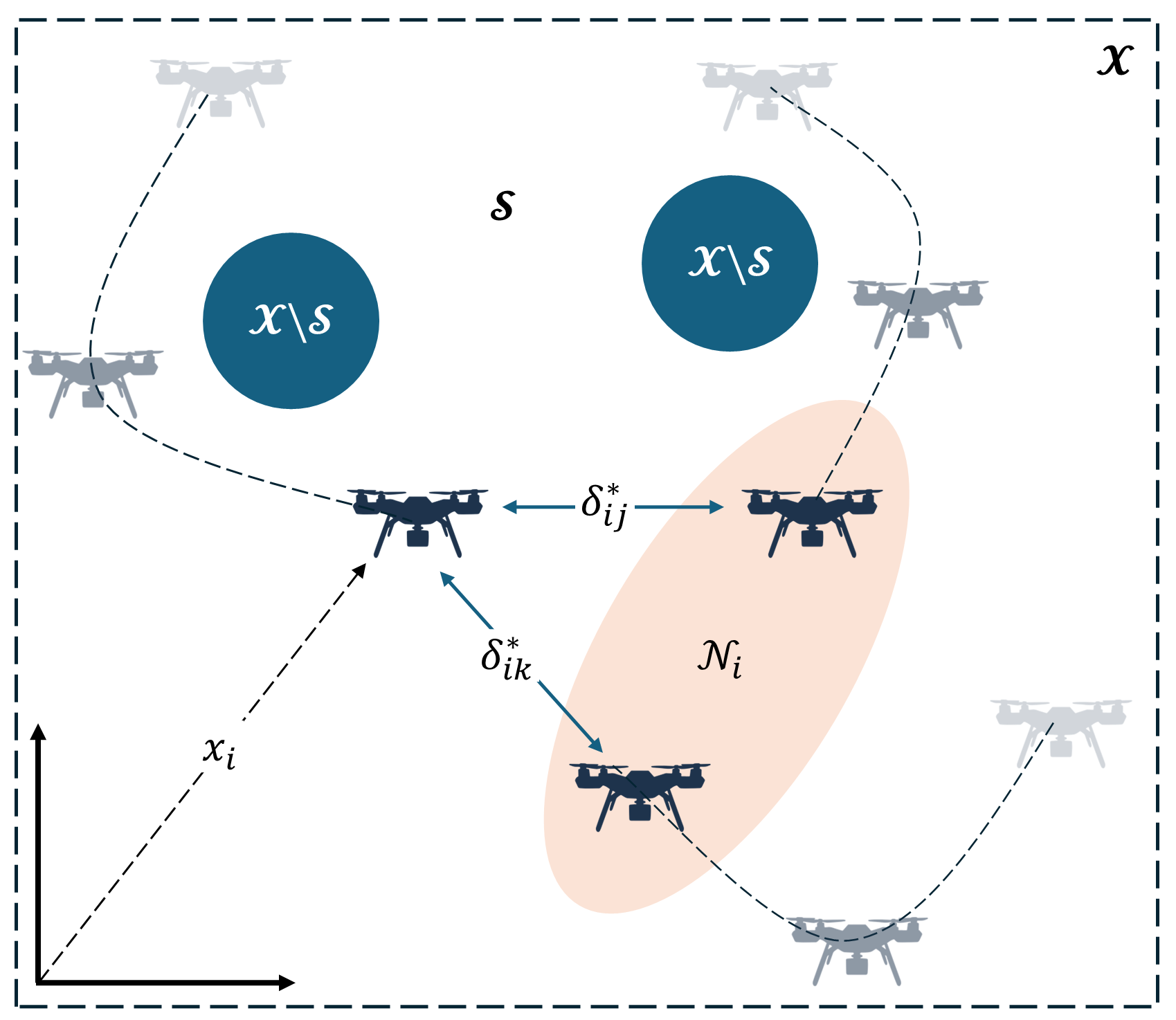
A graph is a pair where is known as the vertex set which contains the vertices or nodes of the graph (i.e. the agents), and is known as the edge set which contains a collection of pairs denoting the connectivity or communication between vertices and of the vertex set. The set of neighbors of node is denoted as .
A graph is called undirected if node communicates with node and vice versa, then . Otherwise, the graph is called directed and node communicates with node but node cannot communicate with node , i.e. . A graph is said to be connected if it has a node to which there exists a (directed) path from every other node. For convenience of the following definitions, throughout this manuscript, only undirected graphs are considered.
Definition 1: The degree matrix of graph is a diagonal matrix whose diagonal entries are equal to the number of neighbors of agent , i.e. 111 denotes the cardinality of the set..
Definition 2: The adjacency matrix of graph is a matrix whose diagonal entries are zero and the off diagonal entries are given by
| (1) |
Definition 3: The Laplacian matrix of graph is defined as
| (2) |
Notice that the sum of the rows and columns of the Laplacian matrix add up to zero, therefore , for all , lies on the right and left null space of . The Laplacian matrix is a symmetric positive semi-definite matrix (). Furthermore, if the graph is connected, the Laplacian has non-zero eigenvalues, i.e. [19].
II-B Control Barrier Functions
Consider a nonlinear control system that is affine in control
| (3) |
where , and are locally Lipschitz, and . Safety can be defined in terms of a continuously differentiable function and a set , such that
| (4a) | |||
| (4b) | |||
| (4c) | |||
The notion of a CBF [20, 21, 22] can be formulated such that its existence allows the system in (3) to be rendered safe with respect to in the sense that the set is made weakly positively invariant for some input . The following definition formalizes this notion.
Definition 4 [21]: Let be the zero-superlevel set of . The function is a Zeroing Control Barrier Function (ZCBF) for , if there exists an extended class kappa function, , such that for the system (3) it can be obtained that:
| (5) |
for all , where is the Lie derivative of with respect to .
For ease of exposition, the time dependency will not be made explicit going forward unless a new variable is introduced or it is relevant to the presented argument.
III The Control Problem
The problem we consider is this paper is the static formation control of distributed MAS consisting of agents indexed by , in the presence of parametric uncertainties and obstacles, with the goal of ensuring stability and safety. The dynamics of agent are given by
| (6) |
where is the state of the agent, is the control input of the agent. is unknown, is an unknown diagonal matrix with known sign, and is known and it has full column rank. The term corresponds to nonlinearities present in the system where is known, but is unknown. For ease of exposition, we assume that and are independent of ; extensions to the case when they depend on are straightforward. We introduce the following assumptions regarding the unknown parameters and nonlinearities in the dynamics:
Assumption 1: The matrix is diagonal and positive definite, .
Assumption 2: The nonlinearity is a bounded signal for all .
Assumption 3: A constant matrix exist such that
| (7) |
where is a known Hurwitz matrix (Section IV-A1).
In addition to the parametric uncertainties, we assume that the problem has safety considerations in the form of state constraints. We now introduce the following definition that pertains to the safety of MAS.
Definition 5 [12]: A continuously differentiable function is referred as a Graph Control Barrier Function (GCBF) if there exists and a control law for each agent of the MAS, such that
| (8) |
where
| (9) |
for where is the joint state of the agents in neighbor set .
The state constraints are captured by the safe set for each agent which corresponds to the obstacle-free region of the state space. Associated with this safe set is a GCBF , which implies the existence of a in (6) that guarantees (8). We assume that the GCBF satisfies conditions in [23] such that the resulting controller is Lipschitz.
The overall problem statement is therefore the following: given that the initial condition for all and a desired position in the static formation for all , the problem is to find a control policy of the form
| (10) |
that guarantees that for all , and in the presence of unknown parameters. In addition, we require that each control policy of agent must depend only on its own state and the state of neighboring agents , for .
IV A Safe and Stable Adaptive Controller for Static Formation
The controller that we propose includes an adaptive component and a safety filter. In order to guide the adaptive control design, a reference model is suitably chosen. In Section IV-A, we design such a reference model, the corresponding adaptive controller, and show that the adaptive controller can enable the MAS to reach a desired formation. In Section IV-B, we integrate a safety filter into the whole adaptive control design and show that the desired formation can be reached even while ensuring the safety constraints. The corresponding results are stated in Theorem 2, Corollary 1, and Theorem 3.
IV-A Stable Formation Control
IV-A1 Reference Model
The starting point for the adaptive solution to the MAS formation control is the choice of a reference model which specifies the desired trajectory that the MAS should follow. For this purpose, we propose a reference model dynamics similar to that in [24, 25]:
| (11a) | |||
| (11b) | |||
where is the state of the reference model , is a Hurwitz matrix, is the reference input vector, and is a constant control gain. The choice of is dictated by the static formation that is of interest. The gain ensures that the closed-loop reference system remains stable, for a given graph .
The following theorem clarifies the conditions under which the reference model (11a), (11b) leads to the desired formation [25].
Theorem 1 [25]: If the graph that captures the communication among agents () is connected, i.e. , then a choice of
| (12) |
where is the solution of
| (13a) | |||
| (13b) | |||
for a given , and a choice of the reference input
| (14) |
for all , where , ensures that converges to the desired formation , for all .
Remark 1: The result of Theorem 1 holds if the communication graph () varies with time as long as it remains connected.
IV-A2 Adaptive Controller
The input in (6) is determined using an adaptive control approach:
| (15) |
where for are time-varying parameters that are adjusted. Defining the following unknown parameters:
| (16) |
| (17) |
where and , we make the following important observations about the controller in (15). First, it satisfies the communication constraints in (10). Second, a choice of , for all and , guarantees that the closed-loop system specified by the plant in (6) and the controller in (15) matches the reference model in (11a)-(11b). The adjustable parameters are introduced for different purposes: is utilized for stabilizing the linear dynamics, is used to enable convergence to the desired formation, while is used to compensate for the nonlinearities.
We propose the adaptive laws:
| (18a) | |||
| (18b) | |||
| (18c) | |||
where , for all , and a is chosen so that
| (19a) | |||
| (19b) | |||
where is given by (13a).
We now state the first main result of the paper, whose proof can be found in the appendix.
Theorem 2: The closed-loop adaptive system defined by the agent dynamics in (6), the control input (15) and the adaptation laws in (18) has globally bounded solutions for any initial conditions and , for all and . Furthermore converges to the desired final position , for all , as .
Remark 2: The solution for in (19a)-(19b) can be obtained using LMI approaches, with and as decision variables.
We now introduce an important property of this adaptive controller which helps us integrate the CBF-filter in to the control design in order to ensure safety constraints on the state. We define the following variables
| (20) |
| (21) |
where is the joint state of the reference model, is the joint state of the system, and , for all and , are the parameter errors. We then define bounds , , and given by , and . With these bounds, we introduce the following corollary to Theorem 2:
Corollary 1: For any bounded , the following properties of hold:
-
i)
For all , where
(22) and
-
ii)
There exists a finite time such that for any , , for all
Remark 3: Both Corollary 1(i) and 1(ii) follow from the stability properties of the adaptive system. Corollary 1(i) states that is always bounded, while Corollary 1(ii) states that becomes arbitrarily small after a finite time . The corresponding bounds and will be directly leveraged in designing the safety-inducing CBF filter introduced in the next section.
Remark 4: We note that the bound depends on and , which in turn can be estimated from known upper bounds on the unknown parameters and , for all and . This in turn implies that a known bound can be determined. Such a bound will be utilized in the GCBF introduced in the next section.
IV-B Safe and Stable Formation Control
In order to ensure the safety of the closed-loop dynamics, we first consider safety of the reference dynamics in (11a), (11b). That is, we want to ensure that for all if . A choice of a QP-GCBF filter inspired by [22], ensures this safety
| (23) | ||||
where
| (24) |
, is a safety buffer, and is a GCBF that is a function of only the state of agent and the parameters of the obstacle. We denote the solution of (23),(24) as .
Remark 5: It is important to note that the QP-GCBF filter above can be solved in a decentralized manner. This is due to the fact the lumped quantity is used as the decision variable rather than the relative distances , and due to the fact that the GCBF is a function of only the state of agent and the parameters of the obstacle. Together they allow a decentralized solution to the QP-GCBF filter.
We now proceed to address the safety of the actual closed-loop dynamics of (6) with the adaptive controller given by (15)-(19b). For this purpose, we note two points. First, the addition of a safety filter as in (23),(24) produces a new reference rather than the one in (14). Second, Corollary 1 implies that the adaptive system state approaches the reference state and therefore approaches as . In order to account for the difference between the system state and the reference state for all time , we modify the QP-GCBF filter from (23),(24) as follows:
| (25) | ||||
where is such that for all and , for all and , and is any finite constant. is given by (22) and is the Lipschitz constant of . That such finite and exist follows from Theorem 2 and Corollary 1.
The complete integrative safe and stable adaptive controller is given by (15)-(19b), but with (15) and (18b) replaced by a modified control input (26) and a modified adaptive law (27), respectively, which are given by
| (26) |
| (27) |
and is the solution of the modified QP-GCBF filter in (25).
The addition of the larger buffer during the initial transients for guarantees the safety of the adaptive system. This is formally stated in Theorem 3, whose proof can be found in the appendix.
Theorem 3: The closed-loop adaptive system defined by the plant in (6), the reference model (11a), (11b) with replaced by , the solution of the modified QP-GCBF in (25), and the adaptive controller given by (26), (18a), (27), (18c), (19a) and (19b) guarantees that for all , if for all . Further, as if for all .
V Simulation
The proposed controller is applied to a two-dimensional obstacle avoidance problem. The dynamics of each agent are given by
| (28) |
such that and are respectively the horizontal and vertical positions of the agents, actuation has been compromised () and the nonlinearities are characterized by
| (29) |
| (30) |
The reference model is defined by
| (31) |
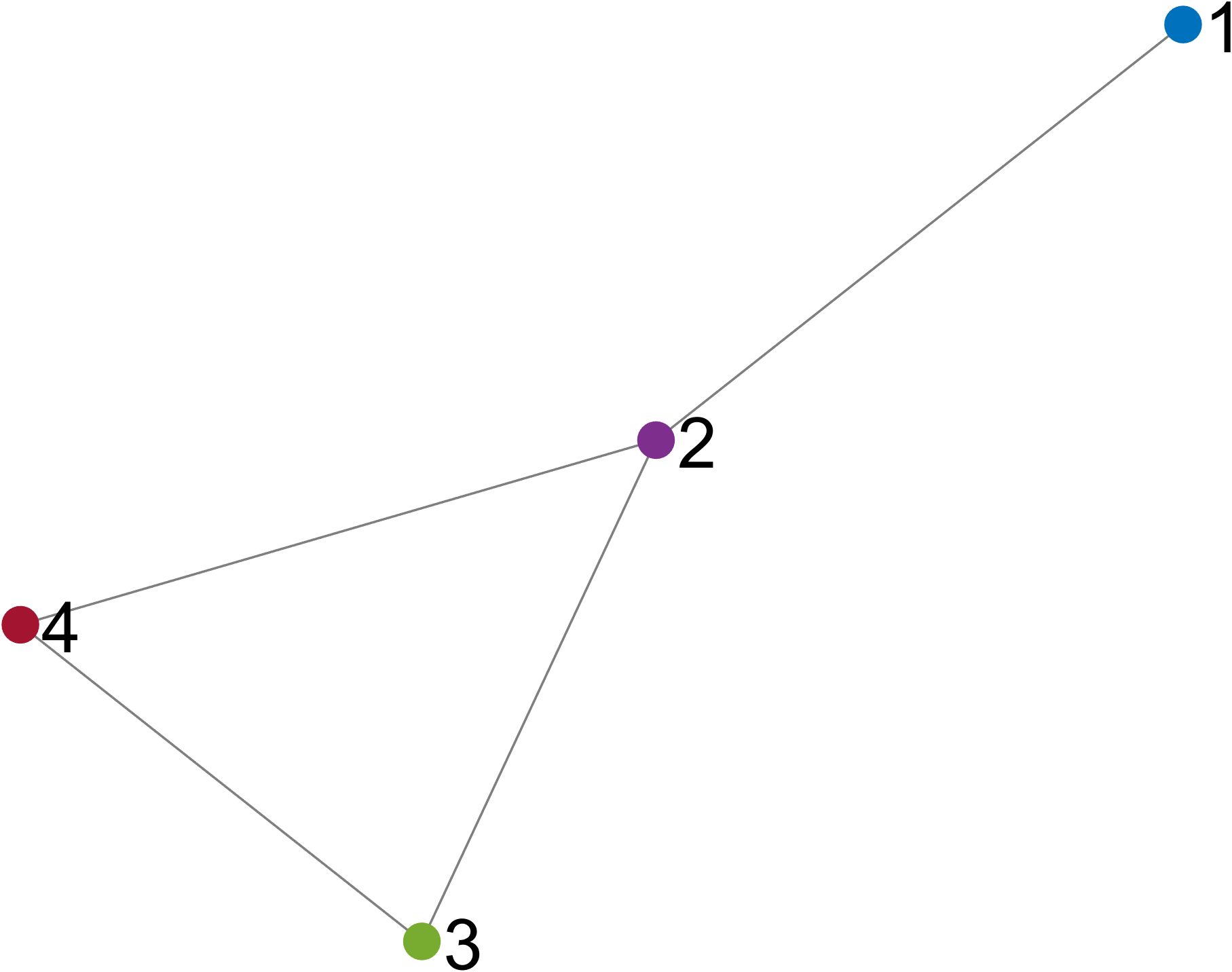
and the communication graph shown in Fig. 2. To guarantee the safety of each agent, the following CBF constraint is chosen for each obstacle
| (32) |
where and are the position and radius of the l-th circular obstacle.
The parameters , for all and , are initialized assuming the agents dynamics are given by
| (33) |
where , , and
| (34) |
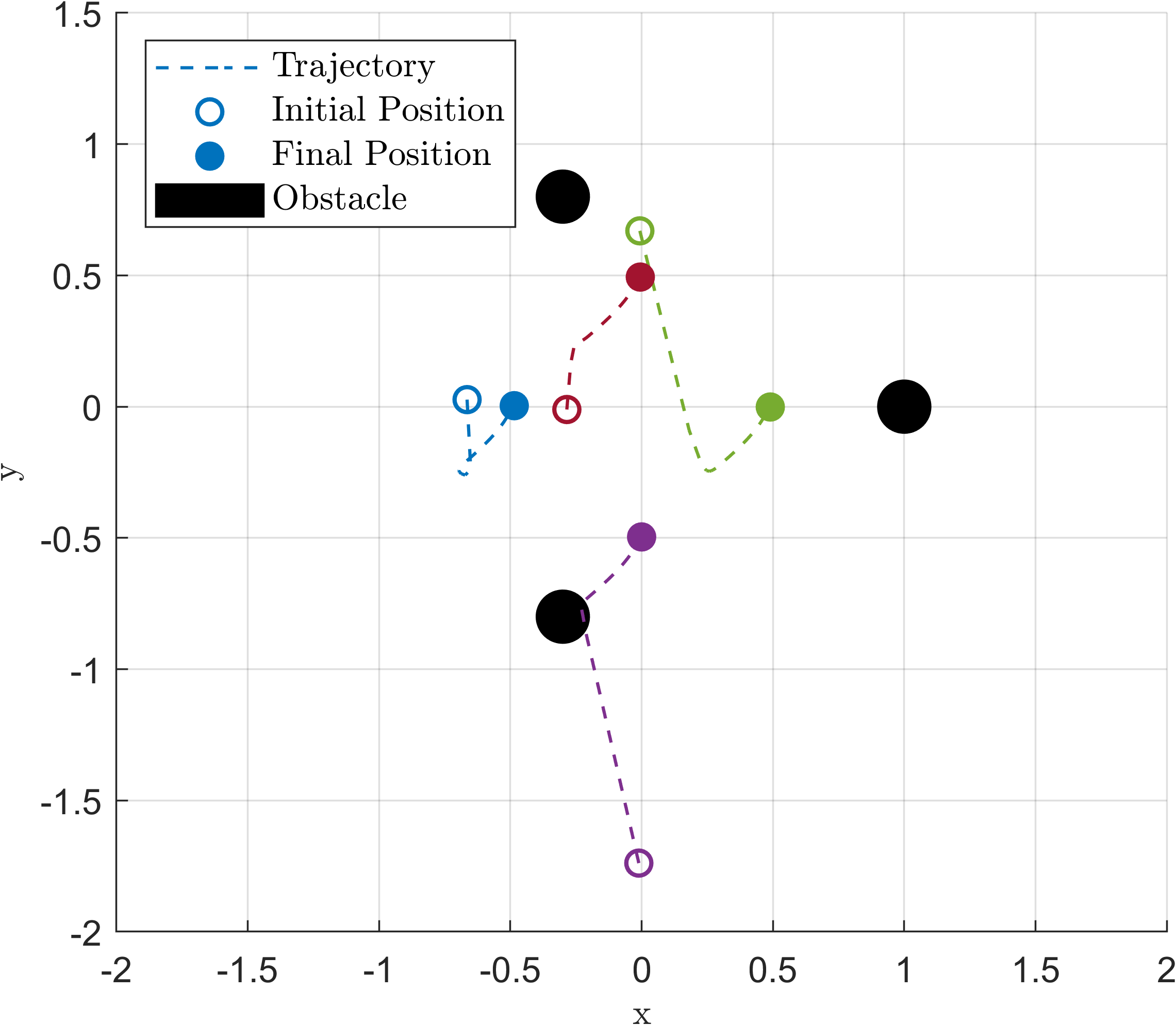
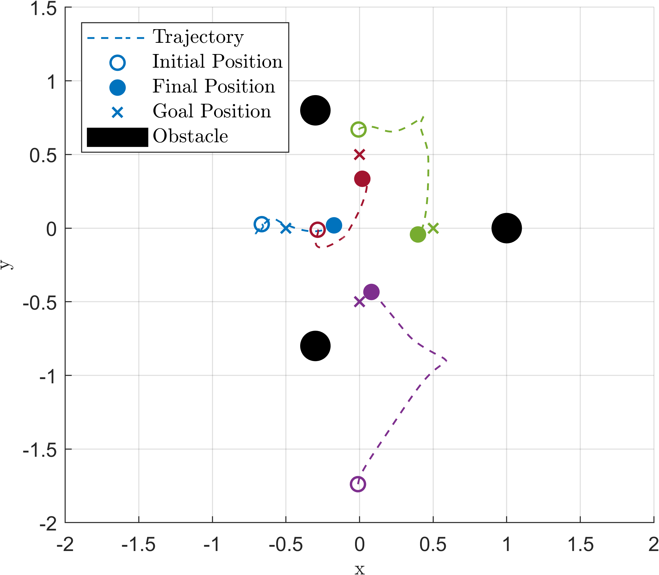
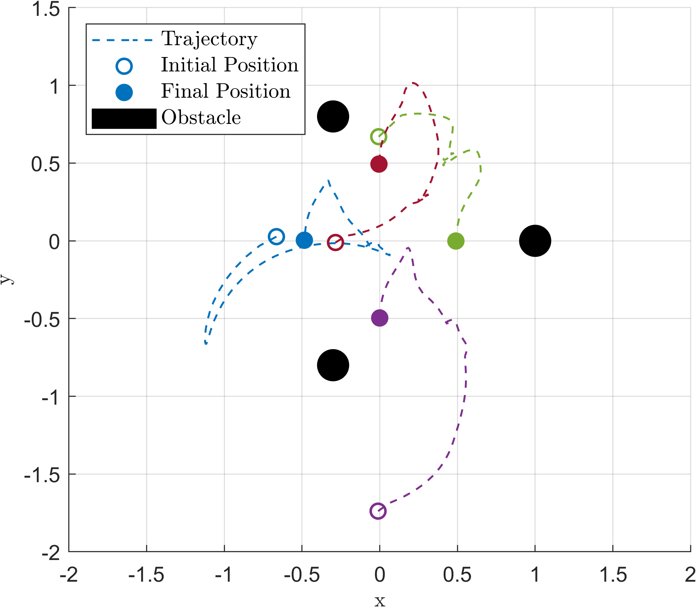
Fig. 3 shows the trajectories of the agents using only the adaptive control described in Section IV-A2 without any safety filter. Fig. 4 shows the trajectories of the agents with the modified QP-GCBF filter in (25) but without adaptation. Finally, Fig. 5 shows our proposed integrative adaptive controller with the modified GCBF and the graph-based reference model as in (11). For the last figure, a , and were chosen. The superior performance of our proposed controller compared with adaptation but no safety as well as safety but with no adaptation is clear from these figures. When the adaptive controller is employed but without any CBF, agent 2 collides with an obstacle along the trajectory (Fig. 3). Only using the modified GCBF but without adaptation allows the MAS to remain safe, but the agents do not reach the desired formation (Fig. 4). In contrast, with our proposed approach in this paper, agents reach the desired formation without collision (Fig. 5). We refer the reader to aaclab.mit.edu for animations of the results. It was observed that a larger , that can be determined using known upper bounds on the parametric uncertainties, led to a more conservative performance with the trajectories staying far from the obstacle during the transient phase of the adaptation.
It’s crucial to emphasize that the system successfully accomplishes the task without collisions, despite operating under unstable dynamics and partially known nonlinearities. Furthermore, it manages to do so even when the actuation is compromised in an unknown manner.
VI Conclusions
In this paper, we consider the problem of static formation control with distributed MAS in the presence of parametric uncertainties and limited communication. The class of problems considered is nonlinear systems that are feedback linearizable, with states accessible for measurement. The goal is to ensure that the MAS stay inside a safe set with the overall closed-loop system remaining stable while meeting the formation goals. Our approach is a combination of adaptive control and control barrier functions, with the former providing a means for accommodating to parametric uncertainties and the latter providing a safety filter that ensures that the states stay within a safe region and remain forward-invariant. The innovations are the design of a GCBF suitably modified to account for parametric uncertainties and the design of a graph-based reference model which serves as a desired dynamics that ensures a safe formation. Theoretical results are provided that guarantee global boundedness and safety against obstacles in the overall state space, and convergence to the desired formation. Numerical results show the effectiveness of the proposed method.
References
- [1] E. Lavretsky, N. Hovakimyan, A. Calise, and V. Stepanyan, “Adaptive Vortex Seeking Formation Flight Neurocontrol,” in AIAA Guidance, Navigation, and Control Conference and Exhibit, (Reston, Virigina), American Institute of Aeronautics and Astronautics, 8 2003.
- [2] Z. T. Dydek, A. M. Annaswamy, and E. Lavretsky, “Adaptive configuration control of multiple UAVs,” Control Engineering Practice, vol. 21, no. 8, pp. 1043–1052, 2013.
- [3] R. Li, L. Zhang, L. Han, and J. Wang, “Multiple Vehicle Formation Control Based on Robust Adaptive Control Algorithm,” IEEE Intelligent Transportation Systems Magazine, vol. 9, no. 2, pp. 41–51, 2017.
- [4] X. Cai and M. d. Queiroz, “Adaptive Rigidity-Based Formation Control for Multirobotic Vehicles With Dynamics,” IEEE Transactions on Control Systems Technology, vol. 23, no. 1, pp. 389–396, 2015.
- [5] N. Xuan-Mung and S. K. Hong, “Robust adaptive formation control of quadcopters based on a leader–follower approach,” International Journal of Advanced Robotic Systems, vol. 16, p. 1729881419862733, 7 2019.
- [6] W. Wang, J. Huang, C. Wen, and H. Fan, “Distributed adaptive control for consensus tracking with application to formation control of nonholonomic mobile robots,” Automatica, vol. 50, no. 4, pp. 1254–1263, 2014.
- [7] L. Dai, Q. Cao, Y. Xia, and Y. Gao, “Distributed MPC for formation of multi-agent systems with collision avoidance and obstacle avoidance,” Journal of the Franklin Institute, vol. 354, no. 4, pp. 2068–2085, 2017.
- [8] A. Wasik, J. N. Pereira, R. Ventura, P. U. Lima, and A. Martinoli, “Graph-based distributed control for adaptive multi-robot patrolling through local formation transformation,” in 2016 IEEE/RSJ International Conference on Intelligent Robots and Systems (IROS), pp. 1721–1728, 2016.
- [9] J. F. Flores-Resendiz, D. Avilés, and E. Aranda-Bricaire, “Formation Control for Second-Order Multi-Agent Systems with Collision Avoidance,” Machines, vol. 11, no. 2, 2023.
- [10] J. Fu, G. Wen, X. Yu, and Z. G. Wu, “Distributed Formation Navigation of Constrained Second-Order Multiagent Systems With Collision Avoidance and Connectivity Maintenance,” IEEE Transactions on Cybernetics, vol. 52, no. 4, pp. 2149–2162, 2022.
- [11] L. Wang, A. D. Ames, and M. Egerstedt, “Safety Barrier Certificates for Collisions-Free Multirobot Systems,” IEEE Transactions on Robotics, vol. 33, no. 3, pp. 661–674, 2017.
- [12] S. Zhang, K. Garg, and C. Fan, “Neural Graph Control Barrier Functions Guided Distributed Collision-avoidance Multi-agent Control,” in Conference on Robot Learning, 2023.
- [13] S. Zhang, O. So, K. Garg, and C. Fan, “GCBF+: A Neural Graph Control Barrier Function Framework for Distributed Safe Multi-Agent Control,” 1 2024.
- [14] Y. Zhou, F. Lu, G. Pu, X. Ma, R. Sun, H. Y. Chen, and X. Li, “Adaptive Leader-Follower Formation Control and Obstacle Avoidance via Deep Reinforcement Learning,” in 2019 IEEE/RSJ International Conference on Intelligent Robots and Systems (IROS), pp. 4273–4280, 2019.
- [15] A. Parvareh, M. Naderi Soorki, and A. Azizi, “The Robust Adaptive Control of Leader–Follower Formation in Mobile Robots with Dynamic Obstacle Avoidance,” Mathematics, vol. 11, no. 20, 2023.
- [16] X. Yang and X. Fan, “A Distributed Formation Control Scheme with Obstacle Avoidance for Multiagent Systems,” Mathematical Problems in Engineering, vol. 2019, p. 3252303, 2019.
- [17] X. Ge, Q. L. Han, J. Wang, and X. M. Zhang, “A Scalable Adaptive Approach to Multi-Vehicle Formation Control with Obstacle Avoidance,” IEEE/CAA Journal of Automatica Sinica, vol. 9, no. 6, pp. 990–1004, 2022.
- [18] Q. Shi, T. Li, J. Li, C. L. P. Chen, Y. Xiao, and Q. Shan, “Adaptive leader-following formation control with collision avoidance for a class of second-order nonlinear multi-agent systems,” Neurocomputing, vol. 350, pp. 282–290, 2019.
- [19] R. Merris, “Laplacian matrices of graphs: a survey,” Linear Algebra and its Applications, vol. 197-198, pp. 143–176, 1 1994.
- [20] S. Prajna and A. Jadbabaie, “Safety Verification of Hybrid Systems Using Barrier Certificates,” in Hybrid Systems: Computation and Control (R. Alur and G. J. Pappas, eds.), (Berlin, Heidelberg), pp. 477–492, Springer Berlin Heidelberg, 2004.
- [21] A. D. Ames, J. W. Grizzle, and P. Tabuada, “Control barrier function based quadratic programs with application to adaptive cruise control,” in 53rd IEEE Conference on Decision and Control, pp. 6271–6278, 2014.
- [22] J. Autenrieb and A. Annaswamy, “Safe and Stable Adaptive Control for a Class of Dynamic Systems,” in 2023 62nd IEEE Conference on Decision and Control (CDC), pp. 5059–5066, 2023.
- [23] M. Alyaseen, N. Atanasov, and J. Cortes, “Continuity and Boundedness of Minimum-Norm CBF-Safe Controllers,” 6 2023.
- [24] R. Olfati-Saber and R. M. Murray, “Consensus problems in networks of agents with switching topology and time-delays,” IEEE Transactions on Automatic Control, vol. 49, no. 9, pp. 1520–1533, 2004.
- [25] Z. Li, Z. Duan, G. Chen, and L. Huang, “Consensus of Multiagent Systems and Synchronization of Complex Networks: A Unified Viewpoint,” IEEE Transactions on Circuits and Systems I: Regular Papers, vol. 57, no. 1, pp. 213–224, 2010.
- [26] R. Bellman, Introduction to Matrix Analysis, Second Edition. Society for Industrial and Applied Mathematics, second ed., 1997.
- [27] K. S. Narendra and A. M. Annaswamy, Stable adaptive systems. USA: Prentice-Hall, Inc., 1989.
-A Proof of Theorem 2
The error dynamics can be written as:
| (36) |
where
| (37) |
| (38) |
| (39) |
We consider the following Lyapunov function candidate:
| (40) |
where , since and is given by (19). This choice for is motivated by the fact that it not only needs to guarantee that the system is stable but also needs to ensure that the adaptive laws are only a function of the state of agent and the state of its neighbors .
With this choice of and adjusting the control gains as in (18), it can be shown (using the properties of the Kronecker product[26], (19b), and standard adaptive control arguments [27]) that
| (41) |
Since is positive definite and radially unbounded and is negative semidefinite, then , for all and . Furthermore, because we have that , and since , by Barbalat’s Lemma we are able to conclude that .
-B Proof of Theorem 3
The construction of the modified QP-GCBF filter implies that its solution is piecewise continuous and bounded. As a result, the conclusions of Corollary 1(i) and 1(ii) hold.
The QP-GCBF filter also guarantees that the reference model solutions are safe. That is, for any , for all . Also implies whenever or . That in turn implies that for all and , which implies that for all and , proving the theorem.