Rotating regular black holes and other compact objects with a Tolman type potential as a regular interior for the Kerr metric

Inspired in the work by Tolman [62], we consider the metric potential $f(r)$ of the static spherically symmetric spacetime (4) in the form

where $R$ and $A$ are two arbitrary constant parameters. This is the Tolman metric potential associated to his type-VII solution.

The metric (4), with $f(r)$ given by (6), is a solution of the Einstein equations whose source is an anisotropic fluid. Such a fluid is characterized by the energy density $\rho$, radial pressure $p_{r}$, and tangential pressure $p_{t}$ given by the expressions

The energy density given by equation (7) vanishes at $r_{v}=\sqrt{\frac{3}{5}}\frac{A^{2}}{R}$. Therefore, we restrict the analysis of the fluid quantities to the region $r\leq r_{v}$.

Notice that, while Tolman dealt just with perfect fluid models, the present model represents a nonperfect fluid, i.e., an anisotropic fluid. In fact, the above solution can be viewed also as a particular case of the anisotropic spheres studied in Ref. [64].

With the choice (6), the mass function $M(r)$ is given by

and then the resulting interior solution is the stationary metric (1) with $M(r)$ given by (10).

The exterior spacetime is described by the Kerr metric which, in the Boyer-Lindquist coordinates, is given by (1) with a constant mass function, i.e., with

The exterior Kerr metric is to be smoothly matched to the interior metric considered in Sec. III.1.

The goal of this section is finding the smooth junction conditions between the exterior Kerr metric and the interior axisymmetric metric. For this end we employ the Darmois-Israel [65] matching conditions, see also Drake and Turolla [44] for and interesting example of application of these junction conditions to stationary spacetimes.

As a first step, we need to identify the boundary surface $S$ that separates the interior region from the exterior region of the spacetime. Such a surface is chosen to be $S:r=r_{0}=$ constant, which is the simplest choice also suggested in Refs. [37, 43] and [44]. Hence, the interior region is defined by values of the radial Boyer-Lindquist coordinate $r$ such that $r<r_{0}$, while the exterior region, where the Kerr metric applies, is for $r$ in the interval $r_{0}<r<\infty$.

The next step is to assume that the transition between the two solutions is smooth, what requires that the first fundamental form on $S$ (the projection of the metric tensor at $r=r_{0}$) and that the second fundamental form (the extrinsic curvature tensor of $S$) be continuous functions across the boundary. Such conditions avoid singular energy-momentum tensor at the matching surface (for more details see Ref. [44]). Thus, with the interior and exterior metrics given by the line element (1), the smooth matching conditions imply the mass function $M(r)$ must be at least $C^{1}$. As a result of these assumptions, the boundary conditions become

where $M_{in}$ stands for the inner mass function, given by Eq. (10), while $M_{Kerr}$ denotes the exterior mass parameter, related to Eq. (11). See Appendix A for more details. The two relations in (12) imply the constraints

so that the complete solution is given by the line element (1) with the mass function in the form

where $\Theta(x)$ is the step (Heaviside) function.

Notice that the radius of the matching surface coincides with the radius where the energy density (7) vanishes. As seen in the previous section, the energy density reaches zero value at $r_{v}=\sqrt{\frac{3}{5}}\frac{A^{2}}{R}$. Moreover, by using the second relation in Eq. (13), it follows $r_{v}^{2}=\frac{3}{5}\frac{A^{4}}{R^{2}}=r_{0}^{2}$. The vanishing of the energy density exactly at the boundary surface is a consequence of the equation of state, $\rho(r)=-p_{r}(r)$, and of the smooth boundary conditions imposed here, what implies in $p_{r}(r_{0})=0=\rho(r_{0})$. This can be seen from Eqs. (7) and (8) (See also the next section for the analysis of the energy density and pressure of the rotating fluid).

The present model has five constant parameters, namely, $R$, $A$, $r_{0}$, $m$, and $a$, and two constraints between them given by Eq. (13). Hence, only three of them are free parameters. Here we choose to work with $m,\,a,$ and $r_{0}$ as the relevant free parameters. Moreover, without loss of generality, all parameters carrying dimensions of length may be normalized by $r_{0}$. Therefore, in the numerical analysis, we take $m/r_{0}$, $a/r_{0}$ as the true free parameters of the model.

In order to investigate the properties of the solution, we study the behavior of the curvature scalars related to the spacetime metric (1), with the mass $M(r)$ defined in Eq. (14). Besides, looking for the existence of rotating regular black holes, we investigate the presence of horizons and ergospheres as well. The energy conditions are also analyzed next.

Here we follow Ref. [37] to verify that the matter source for the spacetime geometry (1) is an anisotropic fluid that can be cast into the form

where $\{u^{\mu},\,e_{r}^{\mu},\,e_{\theta}^{\mu},\,e_{\phi}^{\mu}\}$ is an orthornormal tetrad basis given by

in which the plus ($+$) sign goes for positive $\Delta(r)$, while the minus ($-$) sign goes for negative $\Delta(r)$, respectively. In spacetime regions where $\Delta(r)$ is positive, the plus sign is chosen and it results that $u^{\mu}$ is a timelike vector while the remaining are spacelike vectors. In spacetime regions where $\Delta(r)$ is negative, the minus sign has to be chosen and the vectors $u^{\mu}$ and $e_{r}^{\mu}$ change places, with $e_{r}^{\mu}$ being the timelike vector of the tetrad.

The quantities $\epsilon$, $p_{r}$, $p_{\theta}$, and $p_{\phi}$ are the energy density, the radial, and the tangential pressures of the fluid, respectively, given by the relations

It is straightforward to verify that the energy density $\epsilon$ assumes only nonegative values. For instance, in the equatorial plane ($\theta=\pi/2$) it assumes the maximum value $8\pi\,\epsilon=15m/r_{0}^{3}=3/R^{2}$ at $r=0$, and decreases monotonically as $r$ grows, finally vanishing at the surface $r=r_{0}$. For $\theta\neq\pi/2$, $\epsilon$ vanishes at $r=0$ and at the surface $r=r_{0}$, being finite and positive everywhere else in the interval $0<r<r_{0}$. The vanishing of the energy density at the center in the Boyer-Lindquist coordinates is a feature shared by other models of regular black holes found in the literature (see e.g. Refs. [66] and [67] for other examples of this behavior). Alternative mass functions that lead to a nonvanishing central energy density may cause other problems. This is the case of some of the models discussed in Refs. [47, 53]. Another example is the rotating black hole model presented in Ref. [68]. It has a central core of quintessential matter with nonzero density at $r\to 0$, but the fluid quantities and the curvature scalars present singularities at the region $r=0,\,\theta\neq\pi/2$. As shown in Ref. [69], the Gürses-Gürsey gives rise to singular spacetimes whenever the mass function is finite or goes to zero at $r\to 0$ as $r^{3+n}$ with $n<1$, which is the case of Ref. [68].

Other interesting conditions that a fluid is usually tested for are the standard energy conditions. Here we need to check just the weak energy condition (WEC). The WEC applied to a nonisotropic fluid implies in the constraints $\epsilon\geq 0$ and $\epsilon+p_{i}\geq 0$ ($i=r,\,\theta,\,\phi$) [1]. According to Eq. (17), the energy density satisfies the first constraint in the whole interval $0\leq r\leq r_{0}$ for all $\theta$. The second constraint also holds for the radial $p_{i}=p_{r}$, i.e., one has $\epsilon+p_{r}\geq 0$ in the whole interval $0\leq r\leq r_{0}$ for all $\theta$. On the other hand, as it is seen from Eq. (18), such an inequality does not hold for the tangential pressures $p_{i}=p_{\theta}$ and $p_{i}=p_{\phi}$. In fact, for $\theta\neq\pi/2$, the constraint $\epsilon+p_{\theta}\geq 0$ is satisfied in the interval $r_{b}\leq r\leq r_{0}$, but it is violated close to $r=0$, in the interval $0<r<r_{b}$, where $r_{b}$ is such that $r_{b}^{2}\equiv a^{2}\cos^{2}\theta\left(\sqrt{1+8r_{0}^{2}/a^{2}\,\cos^{2}\theta}-1\right)/2$.

As just analyzed, the present model of rotating compact objects violates the WEC for all $a\neq 0$. This result agrees with Refs. [53, 70, 71], where the authors claim that the addition of rotation into regular blackhole solutions inevitably leads to violation of the WEC. This happens for several rotating regular black holes reported in the literature, see Refs. [47, 55, 72, 73]. In fact, in Ref. [53] it is shown that the black hole rotation unavoidably leads to the violation of the WEC for any physically reasonable choice of the mass function. The energy conditions in the Gürses-Gürsey metric has been considered in some detail in the recent work of Ref. [69]¹¹1This paper by K. Maeda appeared in the arXiv just after the publication of first version of the present manuscript in there.. See also Ref. [74] for a recent short review on rotating regular black holes.

The curvature scalars of the Gürses-Gürsey metric have been analyzed in several works in the literature. Here we mention the recent work by Ref. [69] where it is shown that, among other interesting results, when the mass function $M(r)$ is such that it can be expanded as powers of $r$ close to the region $r=0$, i.e., $M(r)\simeq r^{3+n}$ with $n\geq 0$ (which is the case here), then curvature singularities are absent. The same result was shown in other previous works, see e.g. [53, 71]. To verify this result in the present case, we analyze the relevant curvature invariants (scalars), such as the Ricci scalar $\mathcal{R}=g^{\mu\nu}R_{\mu\nu}$, the Ricci squared $\mathcal{R}_{2}=R_{\mu\nu}R^{\mu\nu}$, and the Kretschmann scalar $\mathcal{K}=R_{\mu\nu\alpha\beta}R^{\mu\nu\alpha\beta}$. For the metric (1), these curvature scalars take, respectively, the forms (see also Ref. [71] for a complete set of curvature scalars for Petrov type D spacetimes).

The Kerr solution is recovered by taking $M^{\prime}(r)=0$, which implies that ${\cal R}$ and ${\cal R}_{2}$ are identically zero, but the Kretschmann scalar is not. In the case of the Kerr spacetime, this scalar diverges at the location where the function $\Sigma=r^{2}+a^{2}\,{\rm cos}^{2}\,\theta$ vanishes, i.e., at $(r,\,\theta)=(0,\,\pi/2)$, what represents a ring-shaped singularity. In other situations, curvature singularities may also occur at the spacetime region where $\Sigma(r,\theta)$ vanishes as it happens for the Kerr metric, even when $M(r)$ and its derivatives are required to be regular functions. However, a careful analysis shows that this is not the case for the metric (1) with the mass function given by Eq. (14). In fact, by approaching the region $r=0$ along the equatorial plane, i.e., by putting $\theta=\pi/2$ and then taking the limit $r\to 0$, the scalar invariants (19) reduce, respectively, to

Additionally, by approaching the region $r=0$ from outside the equatorial plane, that is, $r\to 0$ with $\theta\neq\pi/2$, we have that all the curvature invariants vanish. In fact, for small $r$ we have $M(r)={\cal O}\left(r^{3}\right)$, $M^{\prime}(r)={\cal O}\left(r^{2}\right)$, and $M^{\prime\prime}(r)={\cal O}\left(r\right)$. Then it follows

This means that the curvature invariants have finite values everywhere in the Boyer-Lindquist coordinates, but they are not defined on the ring $(r=0,\,\theta=\pi/2)$. Therefore, we conclude that, differently from the Kerr metric, the spinning geometry generated by the mass function (14) is free of curvature singularities.

Even though the presence of horizons in the Gürses-Gürsey metric for several mass functions $M(r)$ has been considered in previous studies, it is worth presenting here some aspects of the horizon function for the particular case of $M(r)$ given by Eq. (14). Such aspects are useful for the analysis of the causal structure presented below.

In Boyer-Lindquist coordinates, metric (1) presents horizons at the spacetime regions where the function $\Delta(r)$ vanishes. Thus, from Eq. (2) it follows that the horizons radii $r_{i}$ are the real and positive roots of the polynomial equations

with the supplemental conditions that the horizons are determined by the solutions of the first equation when $r_{i}\leq r_{0}$, but are given by the solutions of the second equation when $r_{i}\geq r_{0}$.

A simple analysis shows that each one of the polynomial equations (22) may have two, one, or none real positive roots, depending on the relative values of the free parameters $a$, $m$, and $r_{0}$. The critical case that separates situations with no horizon from situations with two horizons is the extremal case, in which $r_{-}=r_{+}\equiv r_{c}$. In such a case, Eq. (22) yields the extremal mass $m_{c}$,

for $\dfrac{r_{c}}{r_{0}}<1$, and

The extremal mass given by the first solution, i.e., given by (23), applies to the cases in which the double horizon is located in the inner region of the spacetime. This first solution presents a minimum extremal mass given by $m_{c}/r_{0}=12/25=0.48$ at $a=0$. This means that, differently from the Kerr metric, rotating extremal (double horizon) black holes may occur even for rotation parameter smaller than unity. The second solution, given in (24), applies to the cases in which the double horizon is located in the exterior region. More details on this subject are reported in Sec. IV.6.

Figure 1 shows the behavior of $\Delta(r)$ as a function of $r/r_{0}$ for three different values of the ratio $a/m$, namely, $a/m=0$, $a/m=0.6$, and $a/m=1.0$, and five different values of the mass to radius ratio $m/r_{0}$. The dotted lines are associated to the exterior Kerr metric, and are drawn for constant $M(r)$, i.e., for $M(r)=m$, while the solid lines correspond to the complete solution with $M(r)$ given by (14). As seen from the figures, the solid and dotted lines are the same in the vacuum region, i.e., for $r/r_{0}\geq 1$. The intersections of each solid curve with the horizontal axis determine the existence and the position of the horizons $r_{-}$, the smallest root that corresponds to the inner (Cauchy) horizon, and $r_{+}$, the largest root that corresponds to the event horizon.

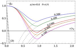
The effects of rotation on the horizon radii may be seen by comparing panel (a) to the other two panels of the same figure. An interesting effect is the increase in the maximum masses of solutions representing regular stars.

Other important surfaces when considering stationary spacetimes are the surfaces of static limit, the so-called ergosurfaces. In the present case, such limiting surfaces correspond to spacetime regions where the Killing vector $\chi^{\mu}=(1,\,0,\,0,\,0)$ becomes lightlike. This condition implies in $g_{tt}=0$, leading to the following equations,

As in the case of the Kerr geometry, these equations may have two real positive roots that define two ergosurfaces that delimit the ergoregions. We denote the two roots by $r_{e^{\pm}}$.

The dependency of the metric coefficient $g_{tt}$ defined in Sec. III as a function of the normalized radial coordinate $r/r_{0}$ is shown in Fig. 2. Each panel is drawn for $\theta=\pi/4$, for a different value of the relative rotation parameter $a/m$, and for a few values of the total mass $m/r_{0}$, as indicated by the line labels. The conventions are the same as in Fig. 1.

The inclusion of rotation makes the surfaces of stationary limit to differ from the horizons, as verified by comparing the curves in panels (a), (b), and (c) of Fig. 2 with the corresponding curves in panels (a), (b), and (c) of Fig. 1, respectively. Also, it is easy to verify that the ergosurfaces may be present in cases where horizons are absent. This happens for rotating configurations with sufficiently high values of the rotation parameter $a/m$ and for masses close to the extremal mass $m_{c}$.

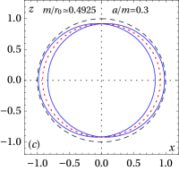
The ergosurfaces of the present stationary spacetime solutions are also displayed in Figs. 3, 4, and 5 by solid blue lines for some values of the parameter $a/m$. The matching surfaces and the horizons (when present) are also shown in that figures respectively by dashed black lines and dotted red lines. A more detailed description of these figures is presented next.

References

- [1] S. W. Hawking and G. F. R. Ellis, The Large Scale Structure of Space and Time (Cambridge University Press, Cambridge, England, 1973).
- [2] J. M. Bardeen, Non-singular general-relativistic gravitational collapse, in Proceedings of GR5 (Tbilisi, URSS, 1968).
- [3] V. P. Frolov, M. A. Markov, and V. F. Mukhanov, Phys. Lett. B 216 (1989) 272.
- [4] I. G. Dymnikova, Gen. Relativ. Gravit. 24 (1992) 235.
- [5] E. Ayón-Beato and A. García, Phys. Rev. Lett. 80 (1998) 5056.
- [6] K. A. Bronnikov, Phys. Rev. D 63 (2001) 044005.
- [7] J. P. S. Lemos, V. T. Zanchin, Phys. Rev. D 83 (2011) 124005.
- [8] S. A. Hayward, Phys. Rev. Lett. 96 (2006) 031103.
- [9] K. A. Bronnikov and J. C. Fabris, Phys. Rev. Lett. 96 (2006) 251101.
- [10] K. A. Bronnikov, R. A. Konoplya, and A. Zhidenko, Phys. Rev. D 86 (2012) 024028.
- [11] J. P. S. Lemos, V. T. Zanchin, Phys. Rev. D 93 (2016) 124012.
- [12] A. Simpson and M. Visser, Universe 6 (2019) 8.
- [13] T. Berry, A. Simpson, and M. Visser, Universe 7 (2020) 2.
- [14] K. A. Bronnikov and J. C. Fabris, Phys. Rev. Lett. 96 (2006) 251101.
- [15] S. Ansoldi, arXiv:0802.0330 [gr-qc].
- [16] Angel D. Masa, Enesson S. de Oliveira, and Vilson T. Zanchin, Phys. Rev. D 103 (2021) 104051.
- [17] R. P. Kerr, Phys. Rev. Lett. 11 (1963) 237.
- [18] S. M. Carroll, Spacetime and Geometry: An Introduction to General Relativity (Addison Wesley, London, England, 2004).
- [19] W. C. Hernandez, Phys. Rev. 159 (1967) 1070.
- [20] J. M. Cohen, J. Math. Phys. 8 (1967) 1477.
- [21] V. De La Cruz and W. Israel, Phys. Rev. 170 (1968) 1187.
- [22] J. B. Hartle and K. S. Thorne, Astrophys. J. 153 (1968) 807.
- [23] P. Florides, Nuovo Cimento 13B (1973) 1.
- [24] P. Florides, Nuovo Cimento 25B (1975) 251.
- [25] W. Israel, Phys. Rev. D 2 (1970) 641.
- [26] V. H. Hamuty, Phys. Lett. A 56 (1976) 78.
- [27] P. Collas and J. K. Lawrence, Gen. Relativ. Gravit. 7 (1976) 715.
- [28] A. Krasinski, Annals Phys. 112 (1978) 22-40.
- [29] F. Z. Majidi, arXiv:1705.00584 [gr-qc].
- [30] N. Uchikata and S. Yoshida, Phys. Rev. D 90 (2014) 064042.
- [31] J. L. Hernandez-Pastora and L. Herrera, Phys. Rev. D 95 (2017) 024003.
- [32] L. Herrera and J. L. Hernandez-Pastora, Phys. Rev. D 96 (2017) 024048.
- [33] A. Simpson and M. Visser, JCAP 03 (2022) 011.
- [34] A. Simpson and M. Visser, Phys. Rev. D 105 (2022) 064065.
- [35] E. T. Newman and A. I. Janis, J. Math. Phys. 6 (1965) 915.
- [36] M. Demiański, Phys. Lett. A 42 (1972) 157-159.
- [37] M. Gürses and F. Gürsey, J. Math. Phys. 16 (1975) 2385.
- [38] G. Clément, Phys. Rev. D 57 (1998) 4885.
- [39] E. N. Glass and J. P. Krisch, Classical Quant. Grav. 21 (2004) 5543.
- [40] S. Viaggiu, Eur. Phys. J. Plus 133 (2018) 551.
- [41] E. Contreras, J. Ovalle, and R. Casadio, Phys. Rev. D 103 (2021) 044020.
- [42] E. T. Newman, R. Couch, K. Chinnapared, A. Exton, A. Prakash, and R. Torrence, J. Math. Phys. 6 (1965) 918.
- [43] L. Herrera and J. Jimenez, J. Math. Phys. 23 (1982) 2339.
- [44] S. P. Drake and R. Turolla, Classical Quant. Grav. 14 (1997) 1883.
- [45] S. P. Drake and P. Szekeres, Gen. Relativ. Gravit. 32 (2000) 445.
- [46] S. Viaggiu, Int. J. Mod. Phys. D 15 (2006) 1441.
- [47] C. Bambi and L. Modesto, Phys. Lett. B 721 (2013) 329-334.
- [48] M. Azreg-Aïnou, Phys. Lett. B 730 (2014) 95-98.
- [49] M. Azreg-Aïnou, Eur. Phys. J. C 74 (2014) 2865.
- [50] M. Azreg-Aïnou, Phys. Rev. D 90 (2014) 064041.
- [51] H. Erbin, Universe 3 (2017) 19.
- [52] B. W. Stewart, J. Phys. A: Math. Gen. 15 (1982) 2419.
- [53] J. C. S. Neves and A. Saa, Phys. Lett. B 734 (2014) 44.
- [54] L. Modesto and P. Nicolini, Phys. Rev. D 82 (2010) 104035.
- [55] B. Toshmatov, B. Ahmedov, A. Abdujabbarov, and Z. Stuchlik, Phys. Rev. D 89 (2014) 104017.
- [56] S. G. Ghosh, Eur. Phys. J. C 75 (2015) 532.
- [57] N. Tsukamoto, Phys. Rev. D 97 (2018) 064021.
- [58] F. Caravelli and L. Modesto, Classical Quant. Grav. 27 (2010) 245022.
- [59] M. Azreg-Aïnou, Class. Quant. Grav. 28 (2011) 148001.
- [60] R. Kumar and S. G. Ghosh, Eur. Phys. J. C 78 (2018) 750.
- [61] S. G. Ghosh, S. D. Maharaj and U. Papnoi, Eur. Phys. J. C 73 (2013) 2473.
- [62] R. C. Tolman, Phys. Rev. 55 (1939) 364.
- [63] A. M. Raghoonundun and D. W. Hobill, Phys. Rev. D 92 (2015) 124005.
- [64] S. D. Maharaj and M. Chaisi, Gen. Relativ. Gravit. 38 (2006) 1723.
- [65] W. Israel, Nuovo Cimento 44B (1966) 1; and corrections in 48B (1967) 463.
- [66] B. Toshmatov, Z. Stuchlík, and B. Ahmedov, Phys. Rev. D 95 (2017) 084037.
- [67] A. Smailagic and E. Spallucci, Phys. Lett. B 688 (2010) 82.
- [68] B. Toshmatov, Z. Stuchlík, and B. Ahmedov, Eur. Phys. J. Plus 132 (2017) 98.
- [69] H. Maeda, JHEP 11 (2022) 108.
- [70] A. Burinskii, E. Elizalde, S. R. Hildebrandt,and G. Magli, Phys. Rev. D 65 (2002) 064039.
- [71] R. Torres and F. Fayos, Gen. Relativ. Gravit. 49 (2017) 2.
- [72] I. Dymnikova and E. Galaktionov, Classical Quant. Grav. 32 (2015) 165015.
- [73] S. G. Ghosh, M. Amir, and S. D. Maharaj, Nucl. Phys. B 957 (2020) 115088.
- [74] R. Torres, “Regular Rotating Black Holes: A Review,” arXiv:2208.12713 [gr-qc].
- [75] P. Beltracchi, P. Gondolo, and E. Mottola, Phys. Rev. D 105 (2022) 024001.
- [76] C. Barrabès and W. Israel, Phys. Rev. D 43 (1991) 1129.