Role of bias and tunneling asymmetries in
nonlinear Fermi-liquid transport
through an SU() quantum dot
Abstract
We study how bias and tunneling asymmetries affect nonlinear current through a quantum dot with discrete levels in the Fermi liquid regime, using an exact low-energy expansion of the current derived up to terms of order with respect to the bias voltage. The expansion coefficients are described in terms of the phase shift, the linear susceptibilities, and the three-body correlation functions, defined with respect to the equilibrium ground state of the Anderson impurity model. In particular, the three-body correlations play an essential role in the order term, and their coupling to the nonlinear current depends crucially on the bias and tunnel asymmetries. The number of independent components of the three-body correlation functions increases with the internal degrees of the quantum dots, and it gives a variety in the low-energy transport. We calculate the correlation functions over a wide range of electron fillings of the Anderson impurity model with the SU() internal symmetry, using the numerical renormalization group. We find that the order nonlinear current through the SU() Kondo state, which occurs at electron fillings of and for strong Coulomb interactions, significantly varies with the three-body contributions as tunnel asymmetries increase. Furthermore, in the valence fluctuation regime toward the empty or fully occupied impurity state, a sharp peak emerges in the coefficient of current in the case at which bias and tunneling asymmetries cooperatively enhance the charge transfer from one of the electrodes.
I Introduction
The ground state and low-lying excited states of quantum-impurity systems [1, 2] such as dilute magnetic alloys and quantum dots can be described as a local Fermi liquid [3, 4, 5, 6, 7], in which localized electrons with discrete energies are strongly coupled to conductions electrons in host metals or electrodes. These low-energy states continuously evolve as the occupation number of the discretized states varies, and various interesting phenomena such as the Kondo effects and the valence fluctuations occur, depending on electron fillings and the configurations [8, 9, 10].
After early observations of the Kondo effect in quantum dots [11, 12, 13, 14, 15, 16, 17], universal Fermi-liquid behaviors were explored through highly sensitive measurements [18, 19, 20, 21, 22, 23] and precise calculations [24, 25, 26, 27]. Furthermore, various kinds of internal degrees of freedom bring an interesting variety to the Kondo effects in quantum dots, such as the one with the SU() symmetry that can be realized in multiorbital dots and in carbon-nanotube (CNT) dots [28, 29, 30, 31, 32, 33, 34, 35, 36, 37, 38, 39, 40, 41, 42, 43, 44]. External magnetic fields also induce interesting crossover phenomena, such as the one between the SU(4) and SU(2) Kondo states observed in a CNT quantum dot [45, 46, 47, 48].
Recent development in the Fermi-liquid theory also reveals that the three-body correlations of electrons passing through the quantum dot play an essential role in the next-leading order terms of the transport coefficients [49, 50, 51, 52, 53] when the system does not have both electron-hole and time-reversal symmetries. This is because, in addition to the well-studied damping of order , , and , quasiparticles of the local Fermi liquid capture the energy shift of the same quadratic order which is induced by the three-body correlations, at low but finite frequencies , temperatures , and bias voltages . The three-body contributions have also been confirmed experimentally in magnetoconductance and nonlinear thermocurrent spectroscopy measurements very recently [54, 55].
Here we focus on the effects of bias and tunneling asymmetries on the nonlinear current at low energies. Specifically, we examine the bias asymmetry that can be described by the parameter , with and the chemical potentials of the source () and drain () electrodes, applied such that , and the Fermi level at thermal equilibrium . The other one, tunneling asymmetry, occurs through the difference between the tunnel couplings and for the source and drain electrodes, respectively. In the previous paper, we demonstrated how these asymmetries affect the transport through a quantum dot described by a spin-1/2 Anderson impurity model with no orbital degrees of freedom [56], and showed that the three-body correlations give significant contributions to the order nonlinear current in the valence fluctuation regime, using the numerical renormalization group (NRG) approach.
The purpose of this paper is to clarify how the conjunction of these asymmetries and the internal degrees of freedom, which increases the independent components of the three-body correlation functions, affects low-energy transport in the Fermi-liquid regime. The low-bias expansion of the conductance up to terms order can be described by the Fermi-liquid theory with the three-body correlations, which at zero temperature takes the following form for a quantum dot with discrete levels which include the spin components,
| (1) |
Here, , which depends on tunneling asymmetries. We present the exact formulas for the coefficients and of the multilevel Anderson impurity model which are applicable to arbitrary impurity electron fillings and arbitrary level structures . These coefficients are determined by the phase shift and the other renormalized parameters, including the three-body correlation functions, and depend crucially on the bias and tunneling asymmetries. We show that, for , the three-body correlations between electrons in three different levels also couple to order nonlinear current as well as the other components when there are some extents of bias and/or tunneling asymmetries. Our formula includes the previous results of the other group as some special limiting cases: derived by Aligia for the Anderson model [57, 58], and derived by Mora et al. for the SU() Kondo model [40].
We also calculate and for the SU() symmetric quantum dots with and , using the NRG in a wide range of electron fillings, varying the parameter corresponding to the gate voltage. There emerge different Kondo states in the SU() symmetric case, which can be classified according to the occupation number , , . We find that large Coulomb interaction suppresses charge fluctuations throughout the region of , and it makes the coefficients and less sensitive to the bias asymmetry, whereas the tunneling asymmetry affects these coefficients. In particular, in the SU() Kondo states at electron fillings of and for , the three-body contributions become sensitive to tunnel asymmetries, and it significantly varies the behavior of the order nonlinear current.
In contrast, in the valence fluctuation regime toward the empty or fully occupied impurity state, i.e., at or , both the bias and tunneling asymmetries affect the nonlinear transport. We find that, in these regions, a sharp peak emerges in the coefficient , in the case at which the bias and tunneling asymmetries cooperatively enhance the charge transfer from one of the electrodes.
This paper is organized as follows. In Sec. II, we describe an outline of the microscopic Fermi-liquid theory for the multilevel Anderson model, and derive the low-energy asymptotic form of the differential conductance. Section III shows the NRG results of quasiparticle parameters for SU() and SU() quantum dots. In Secs. IV and V, we show the NRG results for the coefficients and , respectively. Summary is given in Sec. VI.
II Formulation
We consider a quantum dot with -level coupled to two noninteracting leads by using the Anderson Hamiltonian:
| (2) | ||||
| (3) | ||||
| (4) | ||||
| (5) | ||||
| (6) |
Here, for creates an impurity electron with energy , , and is the Coulomb interaction between electrons in the quantum dot. creates an electron with energy in the lead on the left or right (), and it is normalized as . The linear combination of the conduction electron couples to the dot via the tunneling matrix element . It determines the resonance width of the impurity level , with the tunnel energy scale due to the lead , and the density of state of the conduction band with a half-width . We set throughout this paper, and consider the parameter region where the half bandwidth is much greater than the other energy scales, .
II.1 Fermi-liquid parameters
We describe here the definition of the correlation functions that play an essential role in the microscopic Fermi-liquid theory.
The occupation number and the linear susceptibilities of the impurity level can be derived from the free energy:
| (7) | ||||
| (8) |
where , and represents an equilibrium average, with the inverse temperature.
In addition to linear susceptibilities, the nonlinear ones also play an important role away from half filling:
| (9) |
Here, is the imaginary-time ordering operator. This correlation function has the permutation symmetry: We will use hereafter the ground-state values for , and , and thus the occupation number can be deduced from the phase shift through the Friedel sum rule: [6].
The retarded Green’s function also plays a central role in the microscopic description of the Fermi-liquid transport:
| (10) | ||||
| (11) |
represents a nonequilibrium steady-state average taken with the statistical density matrix, which is constructed at finite bias voltages and temperatures , using the Keldysh formalism [59, 60].
The phase shift is related to the value of the Green’s function at the equilibrium ground state as . It also determines the behavior of the equilibrium spectral function in the low-frequency limit. At the Fermi level , it takes the form
| (12) |
Furthermore, the first derivative of is related to the diagonal susceptibility , as
| (13) |
This is a result of a series of exact Fermi-liquid relations, obtained by Yamada-Yosida [see Appendix A].
II.2 Low-energy expansion of nonlinear current
Nonlinear current through quantum dots can be calculated using a Landauer-type formula [59, 60]:
| (14) |
Here, is the Fermi distribution function for the conduction band on . The chemical potentials of the left and right leads are driven from the Fermi energy at equilibrium by the bias voltage: and , with and the parameters which satisfy , i.e., . Asymmetries in tunnel couplings and that in bias voltages can be described, respectively, by the following parameters,
| (15) | ||||
| (16) |
In this work, we have derived the explicit expressions of the coefficients and for the first two nonlinear-response terms of in Eq. (1), using the exact low-energy asymptotic form of the spectral function of quantum dots embedded in asymmetric junctions obtained up to terms of order , , and . The derivation is given in Appendix B. Specifically, we will use Eqs. (55) and (56) to clarify the roles of the tunnel and bias asymmetries, which enter through the parameters and , in the nonlinear Fermi-liquid transport.
II.2.1 of an SU() dot with tunnel and bias asymmetries
In this paper, we consider the SU() symmetric case, at which the impurity level has the -fold degeneracy: for . For convenience, we use a shifted impurity energy level, defined by in the following. Note that the system additionally has an electron-hole symmetry at .
The linear susceptibilities have two independent components in the SU() symmetric case, i.e., the diagonal component and the off-diagonal one for These two parameters determine the essential properties of quasiparticles:
| (17) |
Here, is a characteristic energy scale of the SU() Fermi liquid, for instance, the -linear specific heat of impurity electrons is scaled in the form . The Wilson ratio corresponds to a dimensionless residual interaction between quasiparticles [61]: we will use the following rescaled Wilson ratio which is bounded in the range ,
| (18) |
The differential conductance for SU() symmetric quantum dots can be expressed in the following form, scaling the bias voltage by ,
| (19) | ||||
| (20) |
The dimensionless coefficients and , can be deduced from the general formulas given in Eqs. (55) and (56), taking into account the SU() symmetry:
| (21) |
For , this reproduces the previous result obtained by Aligia for the spin-1/2 Anderson model [57, 58]. consists of a linear combination of and , and it identically vanishes when both the tunnel couplings and the bias voltages are symmetrical . The magnitude is determined also by and which can be related to the derivative of the spectral function , given in Eq. (13): . Furthermore, is an odd function of . Note that depends on the Coulomb interaction only through the real part of the self-energy.
In contrast, given in the following depends on both the real part that determines the high-order energy shifts and imaginary part that destroy phase coherence [62, 63], specifically on the order and terms. The exact formula of the coefficient for order nonlinear current is composed of two parts: and which represent the two-body contribution and three-body one, respectively,
| (22) | ||||
| (23) | ||||
| (24) |
depends on the asymmetry parameters through the quadratic terms, i.e., , , and . Effects of the three-body corrections enter through the dimensionless parameters:
| (25) | ||||
| (26) | ||||
| (27) |
for . In particular, represents the correlation between three different levels which appears for . This component will give no contribution to through Eq. (24) if there is no tunnel or bias asymmetry [44, 64]: and take the following form at ,
| (28) | ||||
| (29) |
When both the chemical potentials and the tunnel couplings are inverted such that , , , the coefficients and exhibit odd and even properties, respectively: and as shown in Appendix B. These formulas of and of the Anderson model for arbitrary level structures are consistent, in the limit of strong interaction , with the corresponding formulas for the SU() Kondo model obtained by Mora et al. [40] at integer-filling points , with .
III NRG results for Fermi-liquid parameters
In this section, we summarize the basic properties of quasiparticles in the SU() and SU() symmetric cases. Specifically, we have calculated the Fermi-liquid parameters , , and with the NRG approach, dividing channels into pairs, and using the SU() spin and U() charge symmetries for each pair, i.e., totally symmetries. The discretization parameter and the number of low-lying energy states are chosen such that for , and for [44]. The phase shift and renormalized parameters have been deduced from the energy flow of NRG [65, 66, 67, 68, 48].


III.1 SU(4) Fermi-liquid properties
III.1.1 Two-body correlation functions of an SU(4) dot
The Fermi-liquid parameters of an SU(4) quantum dot, which can be deduced from the phase shift and the linear susceptibilities, are shown in Fig. 1 as a function of for several different values of , , , , . For large , the occupation number in Fig. 1(a) shows a Coulomb-staircase behavior with the plateaus of integer height , , and the steps at , , : the structure becomes clearer for stronger interactions. Figure 1(b) shows corresponding to the linear term of the differential conductance in Eq. (1). For strong interactions , the Kondo ridges which reflect the step structure of the occupation number of the values evolve at , respectively, as increases.
Figure 1(c) shows the rescaled Wilson ratio . It has a wide plateau that reaches the strong-coupling limit value in the region , for large interactions . This is caused by the fact that charge fluctuations are suppressed in this region and it makes the charge susceptibility vanish: . The shallow dips of at is caused by the charge fluctuations at the steps of the Coulomb staircase structure of .
Correspondingly, the renormalization factor in Fig. 1(d) exhibits a broad valley structure at , which becomes deeper as increases. It has a clear local minimum for at and , where takes integer values: it also has a local maximum at intermediate valence states in between the two adjacent minima. Figure 1(e) shows the gate voltage dependence of the inverse of the characteristic energy scale, , scaled by that is defined as the value of at the elelctron-hole symmetric point . It shows an oscillatory behavior for strong interactions , reflecting the dependence of on . In particular, reaches a local maximum at the integer-filling points where the SU() Kondo effect occurs.
Some of the two-body correlation functions contribute to the low-energy transport through the derivative of the impurity density of state: given in Eq. (13). For instance, the coefficient is proportional to . Figure 1(f) shows . It is an odd function of and vanishes at where the phase shift takes the value . For strong interactions , it has a wide maximum (minimum) at (), where the -filling (-filling) SU() Kondo occurs.


III.1.2 Three-body correlation functions of an SU(4) dot
We next consider the three-body correlations between electrons passing through an SU(4) symmetric dot. Figure 2 shows , , and as a function of for several different values of . These dimensionless three-body correlation functions vanish in the electron-hole symmetric case . For strong interactions , a plateau of the width emerges at and , i.e., at integer filling points , . The plateau structure evolves further as interaction increases. Specifically, the correlation function between three different levels appears for SU() quantum dots with , and contributes to the nonlinear conductance when there are some asymmetries in the tunnel couplings or the bias voltages.
A comparison of the three independent components , , and is made in Fig. 2(d) for a large interaction . It shows that these three components approach each other very closely over a wide range of gate voltages ,
| (30) |
This is caused by the fact that the derivatives of the two independent components of linear susceptibilities, and , become much smaller than an inverse of the characteristic energy scale in a wide range of electron fillings , in addition to the suppression of the charge fluctuations , mentioned above [see Appendix C] [44].


III.2 SU(6) Fermi-liquid properties
III.2.1 Two-body correlation functions for an SU(6) dot
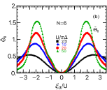
We next summarize the low-energy Fermi-liquid properties of SU() quantum dots. The phase shift and the renormalized parameters that can be deduced from the two-body correlations are plotted as a function of the gate voltage in Fig. 3, for several different values of , , , , i.e., from weak to strong interactions. The behaviors of these parameters are similar to those of the SU() quantum dots. However, the number of different SU() Kondo states occurring at integer fillings increases with , i.e., , , , . It takes place at , , …, , and gives an interesting variety in low-energy transport. As increases, quantum fluctuations caused by the Coulomb interaction is suppressed, and in particular, the mean-field theory becomes exact in the large limit of the finite- Anderson impurity model [69]. Hence for larger , electron-correlation effects occur for stronger interactions .
In Fig. 3(a), we can see that the Coulomb staircase behavior of the occupation number emerges for a large interaction , which has steps at , , for SU() quantum dots. The transmission probability , shown in Fig. 3(b), reaches the unitary limit value at half filling . We can see that the plateau structure develops as increases, and it becomes visible at a strong interaction .
Figure 3(c) shows that the rescaled Wilson ratio for has a wide flat peak at , the height of which increases with . In particular, it approaches saturation value at due to the suppression of charge fluctuations, as mentioned.
The renormalization factor for SU() quantum dots, shown in Fig. 3(d), exhibits a broad valley structure similar to the one for the SU(4) symmetric case. The valley becomes deeper as increases, and the local minima emerge at the integer-filling points, reflecting the electron correlations due to the SU(6) Kondo effects. Figure 3(e) shows that the inverse of the characteristic energy , which is scaled by the value defined at half filling . It has peaks situated at , , for a strong interaction , although the ones at are still developing. These peaks correspond to the SU(6) Kondo temperature at each of the integer-filling points.
Figure 3(f) shows for , which is proportional to the derivative of the density of states , and determines the magnitude of the coefficient of the nonlinear current, as mentioned. This factor is an odd function of , and at a strong interaction it takes a broad peak (dip) at () corresponding to the half-integer filling () where charge fluctuations are not fully suppressed.
III.2.2 Three-body correlation functions of an SU(6) dot
Figure 4 shows three-body correlations between electrons passing through an SU(6) quantum dot, calculated as a function of for several values of interactions , , , . These dimensionless correlation functions , , and vanish at half filling , and away from half filling, they are enhanced as increases. We can see that for a strong interaction there emerges either a wide peak, a wide dip, or a plateau at , , i.e., at integer filling points. The component between three different levels also contributes to the order term of nonlinear current through an SU() quantum dot when there are some asymmetries in the tunnel couplings or the bias voltages.
In Fig. 4(d) the three independent components , , and are compared in a strong interaction case . It shows that these three components approach each other very closely over a wide range of the gate voltage with . This is due to the fact that the diagonal component dominates the three-body correlation, and the derivatives and become much smaller than in a wide range of electron fillings [see Appendix C] [44].
IV Order nonlinear current for SU(4) and SU(6) cases
The coefficient , defined in Eqs. (19) and (21), emerges when the tunnel coupling or the bias voltage is not symmetric. Its magnitude is determined by the Wilson ratio and the derivative of the density of states: .
In this section, we first of all describe behavior of in some limiting cases, and then discuss the NRG results to show how the coefficient evolves with the tunnel and bias asymmetries.
IV.1 Behavior of in some limiting cases
We have seen in Figs. 1 and 3 that the Wilson ratio reaches the saturation value over a wide range of gate voltages for large , where the quantum dot is partially filled . This is caused by the fact that the charge fluctuations are significantly suppressed in this region, as mentioned. In the limit of strong interactions, becomes independent of the bias asymmetry :
| (31) |
In contrast, in the limit of where approaches or , the Wilson ratio approaches the noninteracting value , and becomes independent of tunnel asymmetry :
| (32) |


IV.2
Effects of tunnel asymmetry on
for symmetric bias voltages
We first of all consider effects of tunneling asymmetries on , taking bias voltages to be symmetric :
| (33) |
In this case, is proportional to , and is determined by and . Figure 5 shows as a function of for symmetric bias voltages . We have examined the behaviors from weak to strong interactions: (a) for SU(4) quantum dots with , , , , , and (b) for SU(6) quantum dots with , , , .
As increases, a wide peak and a wide dip of evolve at and , where the occupation number reaches the value of and , respectively. It corresponds to phase shifts of and , at which takes an extreme value as seen in Figs. 1(f) and 3(f). The peak and dip structures also reflect the fact that the Wilson ratio is almost saturated in a wider range of for large in Figs. 1(c) and 3(c). The Kondo effect of an integer filling occurs at the flat peak and the flat dip for quantum dots. In contrast, for , it is an intermediate valence state that occurs at the peak and dip, and thus the structures become round rather than flat since charge fluctuations remain active.
Outside the correlated region, the absolute value of decreases as increases, for both and in Figs. 5 (a) and (b), respectively. In particular, at , it vanishes asymptotically as the occupation number approaches or .


IV.3 Effects of bias asymmetry on
for symmetric tunnel junctions
We next consider the effects of bias asymmetries on , setting tunnel junctions to be symmetric . In this case, becomes proportional to , as
| (34) |
The ratio for this case is plotted vs in Fig. 6. We have also examined from weak to strong interactions for symmetric tunnel couplings : (a) for SU(4) quantum dots with , , , , , and (b) for SU(6) quantum dots with , , , .
At , where the localized levels of quantum dots are partially filled , the factor in Eq. (34) becomes very small as increases since the Wilson ratio approaches the saturation value . Therefore, almost vanishes in this region for strong interactions . However, weak oscillatory behavior survives at for , and it is caused by charge fluctuations in the intermediate valence states between two adjacent integer filling points.
In contrast outside the correlated region, at , the rescaled Wilson ratio decreases and it eventually vanishes in the limit of as shown in Figs. 1(c) and 3(c), so that in Eq. (34). Therefore, the behavior of in this region is mainly determined by the other factor . The localized levels of quantum dots become almost empty or fully occupied in the limit of . Correspondingly, at the crossover region , the phase shift takes the value around at , and at . Thus, the peak height, or the dip depth, of decreases as increases: the amplitude becomes larger for the SU(4) quantum dots than the SU(6) in Fig. 6.
For weak interactions, effects of bias asymmetries appear in the whole region of , particularly takes finite values in the region of .
IV.4 under both asymmetries and
We next consider the behavior of in the presence of both asymmetries, i.e., and . We have seen above that in the strongly correlated region at for large , the coefficient is given by Eq. (31) and it becomes almost independent of bias asymmetries , since the Wilson ratio approaches . Conversely, is given by Eq. (32), which does not depend on tunnel asymmetries , for small or outside the correlated region as . These properties provide the key to clarify overall characteristics of in a wide parameter range.
IV.4.1 Effects of bias asymmetry
on
at large tunnel asymmetry
()
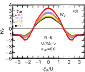
The coefficient for a large fixed tunnel asymmetry , is plotted vs in Fig. 7, varying bias asymmetries, , , . The upper panels describe the behavior for a strong interaction , and the lower ones describe that for weak interactions, i.e., for SU(), and for SU().
The results in Figs. 7 (a) and (b) show that the coefficient becomes almost independent of bias asymmetries in the strong coupling region for large since the Wilson ratio approaches the saturated value . In this region, is proportional to , and shows the same behavior as that in Figs. 5(a) and (b). For , has a peak and a dip which correspond to the points inside the correlated region, and thus the coefficient takes the value at the extreme points. This kind of extreme points in the correlated region do not take place for SU(2) quantum dots since, for , the phase shift takes the values and in the valence fluctuation regime, instead of the Kondo regime [56]. Around the extreme points, takes a typical flat structure of the Kondo state for , while it takes a round structure typical to the intermediate valence state for , as mentioned above.
The coefficient has an additional zero point other than the one at in the case , at which bias and tunneling asymmetries cooperatively enhance the charge transfer from one of the electrodes, and the Wilson ratio satisfies the following condition,
| (35) |
It represents the condition that the first and second terms in Eq. (21) cancel each other out. It takes place valence fluctuation regime in Fig. 7. Conversely, effects of tunnel and bias asymmetries become constructive for . The behavior at , is determined by the factor .


IV.4.2 Effects of tunnel asymmetry
on
at large bias asymmetry
We next consider the effects of tunnel asymmetry on at large bias asymmetry , which describes the situation that the right lead is grounded. Figure 8 shows the result of , plotted as a function varying tunnel asymmetries, as , , , : (top panels) for a strong , and (bottom panels) for weak interactions with (left panels) for SU() quantum dots and (right panels) for SU() ones.
In the strong-coupling limit region , the results in Figs. 8 (a) and (b) show almost the same behavior as that for symmetric bias voltage given in Figs. 5 (a) and (b), respectively, except for the ones for . This is because the Wilson ratio reaches saturated and becomes independent of , as shown in Eq. (31).
In the valence fluctuation region , has an extra zero point other than the one at in the case at which , mentioned above at Eq. (35). As the impurity level deviates further away from the electron-hole symmetric point, i.e., at , the coefficient becomes less sensitive to and its behavior is described by Eq. (32) as the Wilson ratio approaches . We also see in Fig. 8(c) that does not have an extra zero point for SU(4) symmetric quantum dots with a weak interaction. This is because the Wilson ratio in this case takes values in the range as shown in Fig. 1(c) which does not satisfy the condition Eq. (35) as for and . Nevertheless, extra zero points will emerge even in this situation if tunnel asymmetries are slightly larger, i.e., . An example is shown in Fig. 8(d) for SU() quantum dots: has an extra zero point clearly for , whereas it does not for . In this case, the Wilson ratio is bounded in the range of as shown in Fig. 3(c), and thus the condition Eq. (35) is satisfied for at which , whereas it is not, for instance, for as .


V Order nonlinear current for SU(4) and SU(6) cases
The coefficient of the order term of the nonlinear conductance, defined in Eqs. (22)–(24) has a quadratic dependence on the bias and tunnel asymmetries of the form, , , and . In particular, the order term, which is absent in the SU(2) case [70], emerges for multilevel quantum dots with and plays an important role in the Kondo states with no elelctron-hole symmetry. In this section, we describe some limiting cases of , and then discuss the NRG results for SU(4) and SU(6) quantum dots.
V.1 Behavior of in some limiting cases
The two-body and three-body parts of defined in Eqs. (22)–(24) takes the following values in the strong-coupling case where the Wilson ratio reaches the saturated value and the three-body correlations functions show the properties shown in Figs. 1–4,
| (36) | ||||
| (37) |
Our result in this limit is consistent with the corresponding result for the SU() Kondo model, given in Eqs. (22) and (32) of Ref. 40. Note that their notation and our one in the strong-interaction limit correspond to each other such that , and .
In the limit of , the occupation number reaches or , and the correlation functions take the noninteracting values, and thus
| (38) | ||||
| (39) | ||||
| (40) |
Note that in this limit, the three-body correlations are given by , , and [see Appendix B in Ref. 70].


V.2 for symmetric tunnel coupling and symmetric bias voltage
We describe here previous results obtained for symmetric tunnel coupling and bias voltage [53] in order to clarify how the breaking of these symmetries affects the .
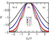
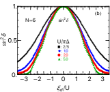
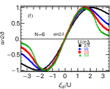
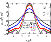
Figures 9(a) and (b) show that , and for as functions of the gate voltage for strong interaction for SU(4) and SU(6) quantum dots. In the strong-coupling limit region , takes plateau structures of the height for SU(4), and for SU(6). In particular, the plateau at half filling, i.e., at , is caused by the two-body correlation . In contrast, the plateau around the Kondo state with the fillings of and , i.e., corresponding to the one electron and one hole occupancies, are caused by the three-body correlation . Specifically, among three independent components defined in Eqs. (25)–(27), determines the peak structure of since owing to the property in the strongly correlated region. In the limit of outside the plateau, the coefficient approaches the noninteracting value , , and , given by Eqs. (38)–(40).
In Figs. 9(c) and (d), for is plotted as a function of , varying interaction strengths (c) , , , , for SU(4), and (d) , , , for SU(6). The plateau structure and the peak at the edge of the plateau of as shown above appear as increases in the strong-coupling limit .
V.3 Effects of tunnel asymmetries on for symmetric bias voltages
We next consider the effect of tunnel asymmetry on , setting bias voltages to be symmetric . In this case, among the three types of quadratic terms , , and in Eqs. (22)–(24), the only term remains finite and contributes to :
| (41) | ||||
| (42) |
The term emerges for . In particular, it couples to , the three-body correlation between electrons in three different levels which does not contribute to for symmetric tunnel couplings.
In the strongly correlated region for large , the three-body part of takes a simplified form which does not depend on , as shown in Eq. (37). Therefore, decreases as tunnel asymmetry which enters through increases, and vanishes at (). In particular, has a wide plateau at the fillings and for large in Fig. 2(b) and Fig. 4(b), the contribution of the three-body correlations becomes significant at these fillings.


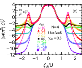
The NRG results of , , and , for the bias symmetric case are plotted vs in the top, upper-middle, and lower-middle panels of Fig. 10, for (left panels) SU(4) and (right panels) SU(6) quantum dots, choosing interaction strength to be . Specifically, Fig. 10 (a)–(f) are obtained, varying tunnel asymmetries, as , , , and . The plateau of emerging at is due to the half-filling Kondo state . The height of this plateau increases with , and approaches the upper bound in the limit . This structure is determined by the two-body part as the three-body part vanishes around the elelctron-hole symmetric point .
We see that the plateau structure of at the Kondo states away from half filling depend sensitively on tunnel asymmetry. The positive plateau emerging at are due to the Kondo state of the filling and . It disappears as increases, and a negative dip develops for . This behavior of reflects the evolution of the three-body part , which is determined by Eq. (37) in the strongly correlated region. Therefore, if is measured varying tunneling asymmetries , the three-body correlation function and can experimentally be deduced, using Eqs. (37) and (42).
In the limit of , the coefficients approach the noninteracting value: , , and for symmetric bias .
Figures 10(g) and (h) compare for several different interaction strengths: (g) , , , , for SU(4), and (h) , , , for SU(6), choosing a large tunnel asymmetry . The dip structure due to the Kondo state at the filling and becomes clear as increases, as well as the plateau due to the half-filling Kondo state.


|

|
V.4 under asymmetric bias voltages
The coefficient depends on the bias and tunnel asymmetries through the terms of order , , and , in Eqs. (23) and (24). We have discussed in the role of the term of the tunnel asymmetry, setting the bias voltages to be symmetric . In this section, we examine the contributions of the other two terms, and .
V.4.1 Effects of bias asymmetry at small and large tunnel asymmetries
In Fig. 11, the coefficient is plotted vs , for (left panels) SU(4) and (right panels) SU(6) quantum dots, varying bias asymmetries , , , and . Specifically, two different tunnel couplings are examined. One (top panels) is the symmetric coupling , at which the role of the term can be clarified. The other one (bottom panels) is a large asymmetric coupling , for which all the quadratic terms, , , and contribute to .
As a large interaction is chosen for each of the panels, the coefficient does not depend on bias asymmetry in the region of , and it takes the values determined by with Eqs. (36) and (37).
In contrast, the coefficient varies with in the valence fluctuation regime . It approaches the asymptotic value which is given by Eq. (40) in the limit of . Since the effect of the bias asymmetry in the tunnel symmetric case is determined by the terms of , the results shown in Figs. 11(a) and (b) do not vary with the sign of the parameter .
In Figs. 11(c) and (d), the coefficient has a sharp peak in the valence fluctuation region at , which grows as bias asymmetry increases. This is caused by the cross term with a positive sign : we will examine the contributions of this term to the peak structures more precisely in the following.


V.4.2 Effects of tunnel asymmetry on at large bias asymmetry
The bias and tunnel asymmetries affect the coefficient through thus quadratic terms , , and in Eqs. (22)–(24). In order to clarify the contribution of the cross term, we set the bias asymmetry to be the upper-bound value , which describes the situation where the bias asymmetry is maximized by grounding the right leads. Therefore, in this case and can be expressed in the following form,
| (43) |
| (44) |
Here, the cross term appears as linear order terms with respect to .
Our discussion here is based on Fig. 12, in which the NRG results of for SU(4) quantum dots and those for SU(6) quantum dots are presented in the left and right panels, respectively. Top panels of Fig. 12 show as a function of the gate voltage , varying tunneling asymmetries , , , , for a strong interaction strength . The upper middle panels show , , for large positive tunnel asymmetries , and correspondingly lower middle panels show the ones for large negative tunnel asymmetries . Bottom panels of Fig. 12 show the results, calculated for several interaction strengths , , , , for SU(4), and , , , for SU(6), taking asymmetric tunnel coupling to be .
In the strongly correlated region for large , the result of in Figs. 12 (a) and (b) almost does not depend on whether or not , and the behavior in this region is determined essentially by the term in Eqs. (36) and (37). The cross term becomes important at , outside the correlated region.
In particular, takes a sharp peak near in the valence fluctuation regime for large positive , i.e., at which bias and tunneling asymmetries cooperatively enhance the charge transfer from one of the electrodes. The results of and , plotted for in Figs. 12 (c)-(d), show the sharp peak structure is mainly due to the three-body part and two-body part has a small constructive peak at the same position. In contrast, for tunnel asymmetry in the opposite direction , each of the two components, and , does not have a peak in Figs. 12 (e)-(f).
We consider more precisely the peak that emerged in the three-body part , taking the limit of in Eq. (44) 111 This limit of strong tunnel asymmetry is meaningful for investigating asymptotic behavior of although it represents the situation where one of the leads is disconnected and the current is determined by Eq. (20).,
| (45) |
Note that each of the three-body correlation functions of the SU() symmetric quantum dots has a definite sign: , , and , as shown in Figs. 2 and 4. Specifically, in the valence fluctuation regime, the positive contribution of in Eq. (45) becomes greater than the negative contribution of , and the difference between these components yields a sharp peak of at . The height measured from the base value of that is defined at the Kondo state in the close vicinity of the valence fluctuation region increases with . Note that in the Kondo state, the three-body correlation functions have a property and in this limit takes a negative value . In the opposite limit of the tunnel asymmetries , the cross term is negative . Therefore, the three-body contribution also becomes negative , and monotonically decreases at .
We also examine how the peak structure evolves with in Figs. 12(g) and (h). The results show that the dip structure in the SU() Kondo regime near and the sharp peak structure in the valence fluctuation regime clearer as interaction increases.
VI Conclusion
We have derived the exact low-bias expansion formula of the differential conductance through a multilevel Anderson impurity up to terms of order , without assuming symmetries in tunnel couplings or bias voltages. It is applicable to a wide class of quantum dots with arbitrary energy level . The expansion coefficients are expressed in terms of the phase shift , linear susceptibilities , and three-body correlation functions , defined with respect to the equilibrium ground state.
The tunnel and bias asymmetries enter the transport coefficients through the parameters and . In contrast to the linear conductance which depends only on the tunnel asymmetry through the prefactor , the nonlinear terms and , given in Eqs. (B.5) and (B.6), depend on both asymmetries. The -dependence enters additionally through the self-energy corrections due to the Coulomb interactions, and the -dependence arises also through a shift of bias window. In particular, emerges when tunnel couplings and/or bias voltages are asymmetrical, and is given by a linear combination of and .
We have explored the behaviors of these coefficients of SU() quantum dots of and with the NRG, in a wide range of parameter space, the varying gate voltage and interaction as well as and . In particular, for large , transport exhibits quite different behaviors depending on electron fillings, especially in the two regions: one is the strongly-correlated region , and the other is the valence fluctuation region in which or . The coefficient of the first nonlinear term of for SU() quantum dots becomes almost independent of bias asymmetries in the strongly-correlated region as charge fluctuation is suppressed in this region. Conversely, it becomes less sensitive to tunnel asymmetries in the valence fluctuation region since interaction effects are suppressed as the filling approaches or .
The three-body correlation functions contribute to the order nonlinear term of , especially in the SU() Kondo regime other than the half-filled one occurring in electron-hole asymmetric cases, and also in the valence fluctuation region. The coefficient of the order term shows the quadratic , and dependences on the bias and tunnel asymmetries.
In particular, the term, which is absent in the SU(2) case, emerges for multilevel quantum dots with , and it couples to a three-body correlation between electrons occupying three different local levels: for . We have found that, as increases, the structure of SU() Kondo plateaus of at and fillings vary significantly from the one for symmetric junctions with . It suggests that the tunnel asymmetries could be used as a sensitive probe for observing three-body correlations in the SU() Kondo states.
The cross term plays an important role, especially in the valence fluctuation region. It yields a sharp peak of when , i.e., in the case at which the tunneling and bias asymmetries cooperatively enhance the charge transfer from one of the electrodes. This is caused by a constructive enhancement of the three-independent components of the three-body correlation function of SU() quantum dots: , , and . Our results indicate that these three-independent components can separately be deduced if is measured varying tunneling asymmetries and bias asymmetries .
Acknowledgements.
This work was supported by JSPS KAKENHI Grant Nos. JP18K03495, JP18J10205, JP21K03415, and JP23K03284, and by JST CREST Grant No. JPMJCR1876. KM was supported by JST, the establishment of university fellowships towards the creation of science technology innovation, Grant Number JPMJFS2138.Appendix A Fermi-liquid relations
The retarded Green’s function defined in Eq. (10) can be expressed in the form,
| (46) |
Specifically, the ground-state properties and the leading Fermi-liquid corrections are determined by the low-frequency behavior of the equilibrium self-energy , or the Green’s function:
| (47) |
Here, the renormalized parameters are defined by
| (48) |
Furthermore, the renormalization factor and the derivative of with respect to the impurity level are related to each other through the Ward identity [4, 7]:
| (49) |
Note that corresponds to an enhancement factor for the linear susceptibilities defined in Eq. (8), i.e., at .
Recently, the Ward identity for the order real part of the self-energy has also been obtained, as [50, 51, 52, 53]
| (50) |
This identity shows that the real part is determined by the intra-level component of the three-body correlation function . Physically, this term of the self-energy induces higher-order energy shifts for single-quasiparticle excitations.
Appendix B Derivation of and
We describe here the derivation of the coefficients and which appeared in Eq. (1). The low-energy asymptotic form of the retarded self-energy for multi-orbital Anderson impurity model was derived up to terms of order , , and in previous work [53, 64],
| (51) |
| (52) |
Here, is a parameter defined in a way such that , and thus
| (53) |
The spectral function can be deduced exactly up to terms of order , , and from the above results of using Eq. (46):
| (54) |
Substituting this low-energy asymptotic form into the the Landauer-type formula in Eq. (14), we obtain the exact expression for the coefficients and for the differential conductance at defined in Eq. (1):
| (55) | ||||
| (56) |
Note that is proportional to the derivative of the density of state as from Eq. (13). The coefficients and have odd and even inversion-symmetrical properties, respectively. Namely, if the left and right leads are inverted together with their tunnel couplings and chemical potentials, sign of changes while does not:
| (57) | |||
| (58) |
Appendix C Behavior of three-body correlation functions for large


In the SU() symmetric case, the two different off-diagonal components and of the three-body correlation functions for can be expressed as a linear combination of the diagonal one and the derivative of the linear susceptibilities [44]:
| (59) | ||||
| (60) |
Figure 13 compares the components emerging on the right-hand side for , i.e., , , and , varying interaction strength . We can see that the diagonal component becomes much larger than the derivative terms and , for strong interactions , over a wide parameter range . Therefore, dominates on the right hand side of Eq. (59) and also on Eq. (60), and thus the corresponding dimensionless parameters show the property described in Eq. (30) for the strong interaction region. We have confirmed that the same behavior occurs in the SU(6) symmetric case.
References
- Kondo [2012] J. Kondo, The Physics of Dilute Magnetic Alloys, edited by S. Koikegami, K. Odagiri, K. Yamaji, and T. Yanagisawa (Cambridge University Press, 2012).
- Hewson [1993] A. C. Hewson, The Kondo Problem to Heavy Fermions (Cambridge University Press, Cambridge, U.K., 1993).
- Nozières [1974] P. Nozières, J. Low Temp. Phys. 17, 31 (1974).
- Yamada [1975a] K. Yamada, Prog. Theor. Phys. 53, 970 (1975a).
- Yamada [1975b] K. Yamada, Prog. Theor. Phys. 54, 316 (1975b).
- Shiba [1975] H. Shiba, Prog. Theor. Phys. 54, 967 (1975).
- Yoshimori [1976] A. Yoshimori, Prog. Theor. Phys. 55, 67 (1976).
- Wilson [1975] K. G. Wilson, Rev. Mod. Phys. 47, 773 (1975).
- Krishna-murthy et al. [1980a] H. R. Krishna-murthy, J. W. Wilkins, and K. G. Wilson, Phys. Rev. B 21, 1003 (1980a).
- Krishna-murthy et al. [1980b] H. R. Krishna-murthy, J. W. Wilkins, and K. G. Wilson, Phys. Rev. B 21, 1044 (1980b).
- Goldhaber-Gordon et al. [1998a] D. Goldhaber-Gordon, H. Shtrikman, D. Mahalu, D. Abusch-Magder, U. Meirav, and M. A. Kastner, Nature 391, 156 (1998a).
- Goldhaber-Gordon et al. [1998b] D. Goldhaber-Gordon, J. Göres, M. A. Kastner, H. Shtrikman, D. Mahalu, and U. Meirav, Phys. Rev. Lett. 81, 5225 (1998b).
- Cronenwett et al. [1998] S. M. Cronenwett, T. H. Oosterkamp, and L. P. Kouwenhoven, Science 281, 540 (1998).
- van der Wiel et al. [2000] W. G. van der Wiel, S. D. Franceschi, T. Fujisawa, J. M. Elzerman, S. Tarucha, and L. P. Kouwenhoven, Science 289, 2105 (2000).
- Schmid et al. [1998] J. Schmid, J. Weis, K. Eberl, and K. v. Klitzing, Physica B: Condens. Matter 256-258, 182 (1998).
- Simmel et al. [1999] F. Simmel, R. H. Blick, J. P. Kotthaus, W. Wegscheider, and M. Bichler, Phys. Rev. Lett. 83, 804 (1999).
- Sasaki et al. [2004] S. Sasaki, S. Amaha, N. Asakawa, M. Eto, and S. Tarucha, Phys. Rev. Lett. 93, 017205 (2004).
- Grobis et al. [2008] M. Grobis, I. G. Rau, R. M. Potok, H. Shtrikman, and D. Goldhaber-Gordon, Phys. Rev. Lett. 100, 246601 (2008).
- Scott et al. [2009] G. D. Scott, Z. K. Keane, J. W. Ciszek, J. M. Tour, and D. Natelson, Phys. Rev. B 79, 165413 (2009).
- Zarchin et al. [2008] O. Zarchin, M. Zaffalon, M. Heiblum, D. Mahalu, and V. Umansky, Phys. Rev. B 77, 241303(R) (2008).
- Delattre et al. [2009] T. Delattre, C. Feuillet-Palma, L. G. Herrmann, P. Morfin, J.-M. Berroir, G. Fève, B. Plaçais, D. C. Glattli, M.-S. Choi, C. Mora, and T. Kontos, Nat. Phys. 5, 208 (2009).
- Yamauchi et al. [2011] Y. Yamauchi, K. Sekiguchi, K. Chida, T. Arakawa, S. Nakamura, K. Kobayashi, T. Ono, T. Fujii, and R. Sakano, Phys. Rev. Lett. 106, 176601 (2011).
- V. Borzenets et al. [2020] I. V. Borzenets, J. Shim, J. C. H. Chen, A. Ludwig, A. D. Wieck, S. Tarucha, H.-S. Sim, and M. Yamamoto, Nature 579, 210 (2020).
- Izumida et al. [2001] W. Izumida, O. Sakai, and S. Suzuki, Journal of the Physical Society of Japan 70, 1045 (2001).
- Oguri [2001] A. Oguri, Phys. Rev. B 64, 153305 (2001).
- Anders [2008] F. B. Anders, Phys. Rev. Lett. 101, 066804 (2008).
- Weichselbaum and von Delft [2007] A. Weichselbaum and J. von Delft, Phys. Rev. Lett. 99, 076402 (2007).
- Laird et al. [2015] E. A. Laird, F. Kuemmeth, G. A. Steele, K. Grove-Rasmussen, J. Nygård, K. Flensberg, and L. P. Kouwenhoven, Rev. Mod. Phys. 87, 703 (2015).
- Borda et al. [2003] L. Borda, G. Zaránd, W. Hofstetter, B. I. Halperin, and J. von Delft, Phys. Rev. Lett. 90, 026602 (2003).
- Izumida et al. [1998] W. Izumida, O. Sakai, and Y. Shimizu, J. Phys. Soc. Japan 67, 2444 (1998).
- Sasaki et al. [2000] S. Sasaki, S. De Franceschi, J. M. Elzerman, W. G. van der Wiel, M. Eto, S. Tarucha, and L. P. Kouwenhoven, Nature 405, 764 (2000).
- Jarillo-Herrero et al. [2005] P. Jarillo-Herrero, J. Kong, H. S. J. van der Zant, C. Dekker, L. P. Kouwenhoven, and S. De Franceschi, Phys. Rev. Lett. 94, 156802 (2005).
- Choi et al. [2005] M.-S. Choi, R. López, and R. Aguado, Phys. Rev. Lett. 95, 067204 (2005).
- Eto [2005] M. Eto, Journal of the Physical Society of Japan 74, 95 (2005).
- Sakano and Kawakami [2006] R. Sakano and N. Kawakami, Phys. Rev. B 73, 155332 (2006).
- Sakano et al. [2007] R. Sakano, T. Kita, and N. Kawakami, Journal of the Physical Society of Japan 76, 074709 (2007).
- Makarovski et al. [2007] A. Makarovski, A. Zhukov, J. Liu, and G. Finkelstein, Phys. Rev. B 75, 241407 (2007).
- Anders et al. [2008] F. B. Anders, D. E. Logan, M. R. Galpin, and G. Finkelstein, Phys. Rev. Lett. 100, 086809 (2008).
- Weymann et al. [2018] I. Weymann, R. Chirla, P. Trocha, and C. P. Moca, Phys. Rev. B 97, 085404 (2018).
- Mora et al. [2009] C. Mora, P. Vitushinsky, X. Leyronas, A. A. Clerk, and K. Le Hur, Phys. Rev. B 80, 155322 (2009).
- Mora [2009] C. Mora, Phys. Rev. B 80, 125304 (2009).
- Cleuziou et al. [2013] J. P. Cleuziou, N. V. N’Guyen, S. Florens, and W. Wernsdorfer, Phys. Rev. Lett. 111, 136803 (2013).
- Mantelli et al. [2016] D. Mantelli, C. P. Moca, G. Zaránd, and M. Grifoni, Physica E 77, 180 (2016).
- Teratani et al. [2020a] Y. Teratani, R. Sakano, and A. Oguri, Phys. Rev. Lett. 125, 216801 (2020a).
- Teratani et al. [2016] Y. Teratani, R. Sakano, R. Fujiwara, T. Hata, T. Arakawa, M. Ferrier, K. Kobayashi, and A. Oguri, J. Phys. Soc. Japan 85, 094718 (2016).
- Ferrier et al. [2016] M. Ferrier, T. Arakawa, T. Hata, R. Fujiwara, R. Delagrange, R. Weil, R. Deblock, R. Sakano, A. Oguri, and K. Kobayashi, Nat. Phys. 12, 230 (2016).
- Ferrier et al. [2017] M. Ferrier, T. Arakawa, T. Hata, R. Fujiwara, R. Delagrange, R. Deblock, Y. Teratani, R. Sakano, A. Oguri, and K. Kobayashi, Phys. Rev. Lett. 118, 196803 (2017).
- Teratani et al. [2020b] Y. Teratani, R. Sakano, T. Hata, T. Arakawa, M. Ferrier, K. Kobayashi, and A. Oguri, Phys. Rev. B 102, 165106 (2020b).
- Mora et al. [2015] C. Mora, C. P. Moca, J. von Delft, and G. Zaránd, Phys. Rev. B 92, 075120 (2015).
- Filippone et al. [2018] M. Filippone, C. P. Moca, A. Weichselbaum, J. von Delft, and C. Mora, Phys. Rev. B 98, 075404 (2018).
- Oguri and Hewson [2018a] A. Oguri and A. C. Hewson, Phys. Rev. Lett. 120, 126802 (2018a).
- Oguri and Hewson [2018b] A. Oguri and A. C. Hewson, Phys. Rev. B 97, 045406 (2018b).
- Oguri and Hewson [2018c] A. Oguri and A. C. Hewson, Phys. Rev. B 97, 035435 (2018c).
- Hata et al. [2021] T. Hata, Y. Teratani, T. Arakawa, S. Lee, M. Ferrier, R. Deblock, R. Sakano, A. Oguri, and K. Kobayashi, Nature Communications 12, 3233 (2021).
- Hsu et al. [2022] C. Hsu, T. A. Costi, D. Vogel, C. Wegeberg, M. Mayor, H. S. J. van der Zant, and P. Gehring, Phys. Rev. Lett. 128, 147701 (2022).
- Tsutsumi et al. [2020] K. Tsutsumi, Y. Teratani, A. Oguri, and R. Sakano, JPS Conf. Proc 30, 011174 (2020).
- Aligia [2011] A. A. Aligia, J. Phys.: Condens. Matter 24, 015306 (2012).
- Aligia [2014] A. A. Aligia, Phys. Rev. B 89, 125405 (2014).
- Hershfield et al. [1992] S. Hershfield, J. H. Davies, and J. W. Wilkins, Phys. Rev. B 46, 7046 (1992).
- Meir and Wingreen [1992] Y. Meir and N. S. Wingreen, Phys. Rev. Lett. 68, 2512 (1992).
- Hewson [2001] A. C. Hewson, J. Phys.: Condens. Matter 13, 10011 (2001).
- Zaránd et al. [2004] G. Zaránd, L. Borda, J. von Delft, and N. Andrei, Phys. Rev. Lett. 93, 107204 (2004).
- Kehrein [2005] S. Kehrein, Phys. Rev. Lett. 95, 056602 (2005).
- Oguri et al. [2022] A. Oguri, Y. Teratani, K. Tsutsumi, and R. Sakano, Phys. Rev. B 105, 115409 (2022).
- Hewson et al. [2004] A. C. Hewson, A. Oguri, and D. Meyer, Eur. Phys. J. B 40, 177 (2004).
- Nishikawa et al. [2010a] Y. Nishikawa, D. J. G. Crow, and A. C. Hewson, Phys. Rev. B 82, 115123 (2010a).
- Nishikawa et al. [2010b] Y. Nishikawa, D. J. G. Crow, and A. C. Hewson, Phys. Rev. B 82, 245109 (2010b).
- Oguri et al. [2011] A. Oguri, R. Sakano, and T. Fujii, Phys. Rev. B 84, 113301 (2011).
- Oguri [2012] A. Oguri, Phys. Rev. B 85, 155404 (2012).
- Tsutsumi et al. [2021] K. Tsutsumi, Y. Teratani, R. Sakano, and A. Oguri, Phys. Rev. B 104, 235147 (2021).
- Note [1] This limit of strong tunnel asymmetry is meaningful for investigating asymptotic behavior of although it represents the situation where one of the leads is disconnected and the current is determined by Eq. (20\@@italiccorr).