RobustNeuralNetworks.jl: a Package for Machine Learning and Data-Driven Control with Certified Robustness
Abstract
Neural networks are typically sensitive to small input perturbations, leading to unexpected or brittle behaviour. We present RobustNeuralNetworks.jl: a Julia package for neural network models that are constructed to naturally satisfy a set of user-defined robustness constraints. The package is based on the recently proposed Recurrent Equilibrium Network (REN) and Lipschitz-Bounded Deep Network (LBDN) model classes, and is designed to interface directly with Julia’s most widely-used machine learning package, Flux.jl. We discuss the theory behind our model parameterization, give an overview of the package, and provide a tutorial demonstrating its use in image classification, reinforcement learning, and nonlinear state-observer design.
keywords:
Julia, Robustness, Machine Learning, Image Classification, Reinforcement Learning, State Estimation1 Introduction
Modern machine learning relies heavily on rapidly training and evaluating neural networks in problems ranging from image classification [He++2016] to robotic control [Siekmann++2021a]. Most neural network architectures have no robustness certificates, and can be sensitive to adversarial attacks and other input perturbations [Huang++2017]. Many that address this brittle behaviour rely on explicitly enforcing constraints during training to smooth or stabilize the network response [Pauli++2022, Junnarkar++2023]. While effective on small-scale problems, these methods are computationally expensive, making them slow and difficult to scale up to complex real-world problems.
Recently, we proposed the Recurrent Equilibrium Network (REN) [Revay++2021b] and Lipschitz-Bounded Deep Network (LBDN) or sandwich layer [Wang+Manchester2023] model classes as computationally efficient solutions to these problems. The REN architecture is flexible in that it includes all common neural network models, such as multi-layer-perceptrons (MLPs), convolutional neural networks (CNNs), and recurrent neural networks (RNNs). The weights and biases in RENs are directly parameterized to naturally satisfy behavioural constraints chosen by the user. For example, we can build a REN with a given Lipschitz constant to ensure its output is quantifiably less sensitive to input perturbations. LBDNs are specializations of RENs with the specific feed-forward structure of deep neural networks like MLPs or CNNs and built-in guarantees on the Lipschitz bound.
The direct parameterization of RENs and LBDNs means that we can train models with standard, unconstrained optimization methods (such as stochastic gradient descent) while also guaranteeing their robustness. Achieving the “best of both worlds” in this way is the main advantage of the REN and LBDN model classes, and allows the user to freely train robust models for many common machine learning problems, as well as for more challenging real-world applications where safety is critical.
This papers presents RobustNeuralNetworks.jl: a package for neural network models that naturally satisfy robustness constraints. The package contains implementations of the REN and LBDN model classes introduced in [Revay++2021b] and [Wang+Manchester2023], respectively, and relies heavily on key features of the Julia language [Bezanson++2017] (such as multiple dispatch) for an efficient implementation of these models. The purpose of RobustNeuralNetworks.jl is to make our recent research in robust machine learning easily accessible to users in the scientific and machine learning communities. With this in mind, we have designed the package to interface directly with Flux.jl [Innes2018], Julia’s most widely-used machine learning package, making it straightforward to incorporate robust neural networks into existing Julia code.
The paper is structured as follows. Section 2 provides an overview of the RobustNeuralNetworks.jl package, including a brief introduction to the model classes (Sec. 2.1), their robustness certificates (Sec. 2.2), and their implementation (Sec. 2.3). Section 3 guides the reader through a tutorial with three examples to demonstrate the use of RENs and LBDNs in machine learning: image classification (Sec. 3.1), reinforcement learning (Sec. 3.2), and nonlinear state-observer design (Sec. LABEL:sec:observer). Section LABEL:sec:conc offers some concluding remarks and future directions for robust machine learning with RobustNeuralNetworks.jl. For more detail on the theory behind RENs and LBDNs, and for examples comparing their performance to current state-of-the-art methods on a range of problems, we refer the reader to [Revay++2021b] and [Wang+Manchester2023] (respectively).
2 Package overview
RobustNeuralNetwork.jl contains two classes of neural network models: RENs and LBDNs. This section gives a brief overview of the two model architectures and how they are parameterized to automatically satisfy robustness certificates. We also provide some background on the different types of robustness metrics used to construct the models.
2.1 What are RENs and LBDNs?
A Lipschitz-Bounded Deep Network (LBDN) is a (memoryless) deep neural network model with a built-in upper-bound on its Lipschitz constant (Sec. 2.2.3). Suppose the network has inputs , outputs , and hidden units . We define LBDNs as -layer feed-forward networks, much like MLPs or CNNs, described by the following recursive equations.
| (1) | ||||
| (2) | ||||
| (3) |
A Recurrent Equilibrium Network (REN) is a neural network model described by linear system in feedback with a nonlinear activation function. Denote as the internal states of the system, as its inputs, and as its outputs. Mathematically, a REN can be written as
| (7) | ||||
| (8) |
where are the inputs and outputs of neurons and is the activation function. Graphically, this is equivalent to Figure 1, where the linear (actually affine) system is given by Equation 7.

See [Revay++2021b] and [Wang+Manchester2023] for more on RENs and LBDNs, respectively.
Remark 1
[Revay++2021b] makes special mention of “acyclic” RENs, which have a lower-triangular matrix. These are significantly more efficient to evaluate and train than a REN with dense matrix, and the performance is similar across a range of problems. All RENs in the current implementation of RobustNeuralNetworks.jl are therefore acyclic RENs.
2.2 Robust metrics and IQCs
All neural network models in RobustNeuralNetworks.jl are designed to satisfy a set of user-defined robustness constraints. There are a number of different robustness criteria which our RENs can satisfy. Some relate to the internal dynamics of the model, others relate to the input-output map. LBDNs are less general, and are specifically constructed to satisfy Lipschitz bounds (Sec. 2.2.3).
2.2.1 Contracting systems
Firstly, all of our RENs are contracting systems. This means that they exponentially “forget” their initial conditions. If the system starts at two different initial conditions but is given the same input sequence, the internal states will exponentially converge over time. Figure 2 shows an example of a contracting REN with one input and a single internal state, where two simulations of the system start with different initial conditions but are provided the same sinusoidal input. See [Bullo2022] for a detailed introduction to contraction theory for dynamical systems.

2.2.2 Incremental IQCs
We define additional robustness criteria on the input-output map of RENs with incremental integral quadratic constraints (IQCs). Suppose we have a model starting at two different initial conditions with two different input signals , and consider their corresponding output trajectories and The model satisfies the IQC defined by matrices if
| (9) |
for some function with , where ,
In general, the IQC matrices can be chosen (or optimized) to meet a range of performance criteria. There are a few special cases that are worth noting.
2.2.3 Lipschitz bounds (smoothness)
If , , for some with , the model satisfies a Lipschitz bound (incremental -gain bound) of , defined by
| (10) |
Qualitatively, the Lipschitz bound is a measure of how smooth the network is. If the Lipschitz bound is small, then small changes in the inputs will lead to small changes in the model output. If is large, then the model output might change significantly for even small changes to the inputs. This can make the model more sensitive to noise, adversarial attacks, and other input disturbances.
As the name suggests, all LBDN models are all constructed to have a user-tunable (or learnable) Lipschitz bound.
2.2.4 Incremental passivity
We have implemented two versions of incremental passivity. In each case, the network must have the same number of inputs and outputs.
-
1.
If where , the model is incrementally passive (incrementally strictly input passive if ). Mathematically, the following inequality holds.
(11) -
2.
If where , the model is incrementally strictly output passive. Mathematically, the following inequality holds.
(12)
For more details on IQCs and their use in RENs, please see [Revay++2021b].
2.3 Direct and explicit parameterizations
The key advantage of the models in RobustNeuralNetworks.jl is that they naturally satisfy the robustness constraints of Section 2.2 – i.e., robustness is guaranteed by construction. There is no need to impose additional (possibly computationally-expensive) constraints while training a REN or an LBDN. One can simply use unconstrained optimization methods like gradient descent and be sure that the final model will satisfy the robustness requirements.
We achieve this by constructing the weight matrices and bias vectors in our models to automatically satisfy specific linear matrix inequalities (see [Revay++2021b] for details). The learnable parameters of a REN or LBDN are a set of free, unconstrained variables . When the set of learnable parameters is exactly , we call this a direct parameterization. Equations 7 to 3 describe the explicit parameterizations of RENs and LBDNs: model structures that can be called and evaluated on data. For a REN, the explicit parameters are , and for an LBDN they are . The mapping depends on the specific robustness constraints to be imposed on the explicit model.
2.3.1 Implementation
RENs are defined by two abstract types in RobustNeuralNetworks.jl. Subtypes of AbstractRENParams hold all the information required to directly parameterize a REN satisfying some robustness properties. For example, to initialise the direct parameters of a contracting REN with 1 input, 10 states, 20 neurons, 1 output, and a relu activation function, we use the following. The direct parameters are stored in model_ps.direct.
[language = Julia] using Flux, RobustNeuralNetworks
T = Float32 nu, nx, nv, ny = 1, 10, 20, 1 model_ps = ContractingRENParamsT( nu, nx, nv, ny; nl=Flux.relu)
println(model_ps.direct) # Access direct params
Subtypes of AbstractREN represent RENs in their explicit form which can be evaluated on data. The conversion from direct to explicit parameters is performed when the REN is constructed and the explicit parameters are stored in model.explicit.
[language = Julia] model = REN(ps) # Create explicit model println(model.explicit) # Access explicit params
Figure 3 illustrates this architecture. We use a similar interface based on AbstractLBDNParams and AbstractLBDN for LBDNs.

2.3.2 Types of direct parameterizations
There are currently four REN parameterizations implemented in this package:
-
1.
ContractingRENParamsparameterizes contracting RENs with a user-defined upper bound on the contraction rate. -
2.
LipschitzRENParamsparameterizes RENs with a user-defined (or learnable) Lipschitz bound of . -
3.
PassiveRENParamsparameterizes incrementally input passive RENs with user-tunable passivity parameter . -
4.
GeneralRENParamsparameterizes RENs satisfying some general behavioural constraints defined by an incremental IQC with parameters (Q,S,R).
There is currently only one LBDN parameterization implemented in RobustNeuralNetworks.jl:
-
1.
DenseLBDNParamsparameterizes dense (fully-connected) LBDNs with a user-defined or learnable Lipschitz bound. A dense LBDN is effectively a Lipschitz-bounded MLP.
We intend to add ConvolutionalLBDNParams to parameterize the convolutional LBDNs in [Wang+Manchester2023] in future iterations of the package.
2.3.3 Explicit model wrappers
When training a REN or LBDN, we learn and update the direct parameters and convert them to the explicit parameters only for model evaluation. The main constructors for explicit models are REN and LBDN.
Users familiar with Flux.jl will be used to creating a model once and then training it on their data. The typical workflow is as follows.
[language = Julia] using Flux
# Define a model and a loss function model = Flux.Chain( Flux.Dense(1 => 10, Flux.relu), Flux.Dense(10 => 1, Flux.relu) )
loss(model, x, y) = Flux.mse(model(x), y)
# Training data of 20 batches T = Float32 xs, ys = rand(T,1,20), rand(T,1,20) data = [(xs, ys)]
# Train the model for 50 epochs opt_state = Flux.setup(Adam(0.01), model) for _in 1:50 Flux.train!(loss, model, data, opt_state) end
When training a model constructed from REN or LBDN, we need to back-propagate through the mapping from direct (learnable) parameters to the explicit model. We must therefore include the model construction as part of the loss function. If we do not, then the auto-differentiation engine has no knowledge of how the model parameters affect the loss, and will return zero gradients. Here is an example with an LBDN, where the model is defined by the direct parameterization stored in model_ps.
[language = Julia] using Flux, RobustNeuralNetworks
# Define model parameterization and loss function T = Float32 model_ps = DenseLBDNParamsT(1, [10], 1; nl=relu) function loss(model_ps, x, y) model = LBDN(model_ps) Flux.mse(model(x), y) end
# Training data of 20 batches xs, ys = rand(T,1,20), rand(T,1,20) data = [(xs, ys)]
# Train the model for 50 epochs opt_state = Flux.setup(Adam(0.01), model_ps) for _in 1:50 Flux.train!(loss, model_ps, data, opt_state) end
2.3.4 Separating parameters and models
For the sake of convenience, we have included the model wrappers DiffREN and DiffLBDN as alternatives to REN and LBDN, respectively. These wrappers compute the explicit parameters each time the model is called rather than just once when they are constructed. Any model created with these wrappers can therefore be used exactly the same way as a regular Flux.jl model, and there is no need for model construction in the loss function. One can simply replace the definition of the Flux.Chain model in the first code cell above with
{lstlisting}[language = Julia]
model_ps = DenseLBDNParamsT(1, [10], 1; nl=relu)
model = DiffLBDN(model_ps)
and train the LBDN just like any other Flux.jl model. We use these wrappers in Sections 3.1 and LABEL:sec:observer.
We must, however, caution against their use in problems where a model is evaluated many times before being updated. The model_ps and model are kept separate with REN and LBDN to offer flexibility. The main computational bottleneck in training a REN or LBDN is converting from the direct to explicit parameters (mapping ). For both model structures, this process involves a matrix inverse, where the number of matrix elements scales quadratically with the dimension of the model in a REN and the dimension of each layer in an LBDN (see [Revay++2021b, Wang+Manchester2023]).
As per Section 2.3.1, direct parameters are stored in model_ps, while explicit parameters are computed when the model is created and are stored within it. In some applications (eg: reinforcement learning), a model is called many times with the same explicit parameters before its learnable parameters are updated. It is therefore significantly more efficient to store the explicit parameters, use them many times, and then update them only when the learnable parameters change. We cannot store the direct and explicit parameters in the same model object since auto-differentiation in Julia does not support array mutation [Innes2018b]. Instead, we separate the two.
Remark 2
The model wrappers DiffREN and DiffLBDN re-compute the explicit parameters every time the model is called. In applications where the learnable parameters are updated after one model call (eg: image classification), it is often more convenient and equally fast to use these wrappers.
In applications where the model is called many times before updating it (eg: reinforcement learning), use REN or LBDN. They compute the explicit model when constructed and store it for later use, making them more efficient.
The computational benefits of separating models from their parameterizations is explored numerically in Section 3.2.
3 Examples
This section guides the reader through a set of examples to demonstrate how to use RobustNeuralnetworks.jl for machine learning in Julia. We will consider three examples: image classification, reinforcement learning, and nonlinear observer design. These examples will provide further insight into the benefits of using robust models and the reasoning behind key design decisions made when developing the package.
We use relu activation functions in all examples, but other choices of activation function (e.g: tanh) are equally valid. We note that any activation function used in a REN or LBDN must have a maximum slope of 1.0, as outlined in [Revay++2021b, Wang+Manchester2023]. For more examples with RENs and LBDNs, please see the package documentation111https://acfr.github.io/RobustNeuralNetworks.jl/.
3.1 Image classification
Our first example features an LBDN trained to classify the MNIST dataset [LeCun++2010]. We will use this example to demonstrate how training image classifiers with LBDNs makes them robust to adversarial attacks thanks to the built-in Lipschitz bound. For a detailed investigation of the effect of Lipschitz bounds on classification robustness and reliability, please see [Wang+Manchester2023].
3.1.1 Load the data
We begin by loading the training and test data. MLDatasets.jl222https://juliaml.github.io/MLDatasets.jl/ contains a number of common machine-learning datasets, including the MNIST dataset. To load the full dataset of 60,000 training images and 10,000 test images, one would run the following code.
[language = Julia] using MLDatasets: MNIST
T = Float32 x_train, y_train = MNIST(T, split=:train)[:] x_test, y_test = MNIST(T, split=:test)[:]
The feature matrices x_train and x_test are three-dimensional arrays where each 28x28 layer contains pixel data for a single handwritten number from 0 to 9 (eg: see Fig. 4). The labels y_train and y_test are vectors containing the classification of each image as a number from 0 to 9. We convert each of these to a format better suited to training with Flux.jl.
[language = Julia] using Flux
# Reshape features for model input x_train = Flux.flatten(x_train) x_test = Flux.flatten(x_test)
# Encode categorical outputs and store y_train = Flux.onehotbatch(y_train, 0:9) y_test = Flux.onehotbatch(y_test, 0:9) data = [(x_train, y_train)]
Features are now stored in a Matrix where each column contains pixel data from a single image, and the labels have been converted to a Flux.OneHotMatrix where each column contains a 1 in the row corresponding to the image’s classification (eg: row 3 for an image showing the number 2) and a 0 otherwise.
3.1.2 Define a model
We can now construct an LBDN model to train on the MNIST dataset. The larger the model, the better the classification accuracy will be, at the cost of longer training times. The smaller the Lipschitz bound , the more robust the model will be to input perturbations (such as noise in the image). If is too small, however, it can restrict the model flexibility and limit the achievable performance [Wang+Manchester2023]. For this example, we use a small network of two 64-neuron hidden layers and set a Lipschitz bound of just to demonstrate the method.
[language = Julia] using RobustNeuralNetworks
# Model specification nu = 28*28 # Inputs (size of image) ny = 10 # Outputs (classifications) nh = fill(64,2) # Hidden layers γ = 5.0f0 # Lipschitz bound 5.0
# Define parameters,create model model_ps = DenseLBDNParamsT(nu, nh, ny, γ) model = Chain(DiffLBDN(model_ps), Flux.softmax)
The model consists of two parts. The first is a callable DiffLBDN model constructed from its direct parameterization, which is defined by an instance of DenseLBDNParams as per Section 2.3. The output is then converted to a probability distribution using a softmax layer. Note that all AbstractLBDN models can be combined with traditional neural network layers using Flux.Chain.
We could also have constructed the model from a combination of SandwichFC layers. Introduced in [Wang+Manchester2023], the SandwichFC layer is a fully-connected or dense layer with a guaranteed Lipschitz bound of 1.0. We have designed the user interface for SandwichFC to be as similar to that of Flux.Dense as possible.
{lstlisting}[language = Julia]
model = Chain(
(x) -> (sqrt(γ) * x),
SandwichFC(nu => nh[1], relu; T),
SandwichFC(nh[1] => nh[2], relu; T),
(x) -> (sqrt(γ) * x),
SandwichFC(nh[2] => ny; output_layer=true, T),
Flux.softmax
)
This model is equivalent to a dense LBDN constructed with LBDN or DiffLBDN. We have included it as a convenience for users familiar with layer-wise network construction in Flux.jl, and recommend using it interchangeably with DiffLBDN.
3.1.3 Define a loss function
A typical loss function for training on datasets with discrete labels is the cross entropy loss. We can use the crossentropy loss function shipped with Flux.jl.
[language = Julia] loss(model,x,y) = Flux.crossentropy(model(x), y)
3.1.4 Train the model
We train the model over 600 epochs using two learning rates: 1e-3 for the first 300, and 1e-4 for the last 300. We use the Adam optimizer [Kingma+Ba2015] and the default Flux.train! method for convenience. Note that the Flux.train! method updates the learnable parameters each time the model is evaluated on a batch of data, hence our choice of DiffLBDN as a model wrapper.
[language = Julia] # Hyperparameters epochs = 300 lrs = [1e-3,1e-4]
# Train with the Adam optimizer for k in eachindex(lrs) opt_state = Flux.setup(Adam(lrs[k]), model) for i in 1:epochs Flux.train!(loss, model, data, opt_state) end end
3.1.5 Evaluate the trained model
Our final model achieves training and test accuracies of approximately 99% and 98%, respectively, as shown in Table 3.1.6. We could improve this further by switching to a convolutional LBDN, as in [Wang+Manchester2023]. Some examples of classifications given by the trained LBDN model are presented in Figure 4.

3.1.6 Investigate robustness
The main advantage of using an LBDN for image classification is its built-in robustness to noise (or attacks) added to the image. This robustness is a direct benefit of the Lipschitz bound. As outlined in the Section 2.2.3, the Lipschitz bound effectively defines how “smooth” the network is: the smaller the Lipschitz bound, the less the network outputs will change as the inputs vary. For example, small amounts of noise added to the image will be less likely to change its classification. A detailed investigation into this effect is presented in [Wang+Manchester2023].
We can demonstrate the robustness of LBDNs by comparing the model to a standard MLP built from Flux.Dense layers. We first create a dense network with the same layer structure as the LBDN.
{lstlisting}[language = Julia]
# Initialisation functions
init = Flux.glorot_normal
initb(n) = Flux.glorot_normal(n)
# Build a dense model dense = Chain( Dense(nu, nh[1], relu; init, bias=initb(nh[1])), Dense(nh[1], nh[2], relu; init, bias=initb(nh[2])), Dense(nh[2], ny; init, bias=initb(ny)), Flux.softmax )
Training the dense model with the same training loop used for the LBDN model results in a model that achieves training and test accuracies of approximately 98% and 97%, respectively, as shown in Table 3.1.6.
Training and test accuracy for the LBDN and Dense models on the MNIST dataset without perturbations. Model structure Training accuracy (%) Test accuracy (%) LBDN 98.7 97.6 Dense 98.4 96.9
As a simple test of robustness, we add uniformly-sampled random noise in the range to the pixel data in the test dataset for a range of noise magnitudes We record the test accuracy for each perturbation size and store it for plotting. {lstlisting}[language = Julia] using Statistics
# Get test accuracy as we add noise uniform(x) = 2*rand(T, size(x)…) .- 1 compare(y, yh) = maximum(yh, dims=1) .== maximum(y.*yh, dims=1) accuracy(model, x, y) = mean(compare(y, model(x)))
function noisy_test_error(model, ϵ) noisy_xtest = x_test .+ ϵ*uniform(x_test) accuracy(model, noisy_xtest, y_test)*100 end
ϵs = T.(LinRange(0, 200, 10)) ./ 255 lbdn_error = noisy_test_error.((model,), ϵs) dense_error = noisy_test_error.((dense,), ϵs)
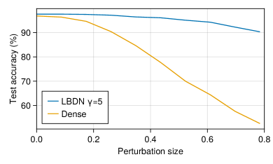
Plotting the results in Figure 5 very clearly shows that the dense network, which has no guarantees on its Lipschitz bound, quickly loses its accuracy as small amounts of noise are added to the image. In contrast, the LBDN model maintains its accuracy even when the (maximum) perturbation size is as much as 80% of the maximum pixel values. This is an illustration of why image classification is one of the most promising use-cases for LBDN models. For a more detailed comparison of LBDN with state-of-the-art image classification methods, see [Wang+Manchester2023].
3.2 Reinforcement learning
One of the original motivations for developing the model structures in RobustNeuralNetworks.jl was to guarantee stability and robustness in learning-based control. Recently, we have shown that with a controller architecture based on a nonlinear version of classical Youla-Kucera parameterization [Youla++1976], one can learn over the space of all stabilising controllers for linear or nonlinear systems using standard reinforcement learning techniques, so long as our control policy is parameterized by a contracting, Lipschitz-bounded REN [Wang++2022, Barbara++2023]. This is an exciting result when considering learning controllers in safety-critical systems, such as in robotics.
In this example, we will demonstrate how to train an LBDN controller with reinforcement learning (RL) for a simple nonlinear dynamical system. This controller will not have any stability guarantees. The purpose of this example is simply to showcase the steps required to set up RL experiments for more complex systems with RENs and LBDNs.
3.2.1 Overview
Consider the simple mechanical system shown in Figure 6: a box of mass sits in a tub of fluid, held between the walls by two springs each with spring constant The box can be pushed with a force Its dynamics are
| (13) |
where is the viscous damping coefficient due to the box moving through the fluid, and denote the velocity and acceleration of the box, respectively.

We can write this as a (nonlinear) state-space model with state control input and dynamics
| (14) |
This is a continuous-time model of the dynamics. For our purposes, we need a discrete-time model. We can discretize the dynamics using a forward Euler approximation to get
| (15) |
where is the time-step. This approximation typically requires a small time-step for numerical stability, but is sufficient for our simple example. If physical accuracy was of concern, one could use a fourth (or higher) order Runge-Kutta scheme.
Our aim is to learn a controller defined by some learnable parameters that can push the box to any goal position that we choose. Specifically, we want the box to:
-
1.
reach a (stationary) goal position
-
2.
within a time period .
The force required to keep the box at a static equilibrium position is from Equation 13. We can encode these objectives into a cost function and write our RL problem as
| (16) |
where , , are cost function weights, and the expectation is over different initial and goal positions of the box.
3.2.2 Problem setup
We start by defining the properties of our system and translating the dynamics into Julia code. For this example, we consider a box of mass , spring constants and a viscous damping coefficient . We will simulate the system over s time horizons with a time-step of s.
[language = Julia] m = 1 # Mass (kg) k = 5 # Spring constant (N/m) μ = 0.5 # Viscous damping (kg/m)
Tmax = 4 # Simulation horizon (s) dt = 0.02 # Time step (s) ts = 1:Int(Tmax/dt) # Array of time indices
Now we can generate the training data. Suppose the box always starts at rest from the zero position, and the goal position can be anywhere in the range . Our training data consists of a batch of 80 randomly-sampled goal positions and corresponding reference forces . {lstlisting}[language = Julia] nx, nref, batches = 2, 1, 80 x0 = zeros(nx, batches) qref = 2*rand(nref, batches) .- 1 uref = k*qref
It is good practice (and faster) to simulate all simulation batches at once, so we define our dynamics functions to operate on matrices of states and controls. Each row corresponds to a different state or control, and each column corresponds to a simulation for a particular goal position. {lstlisting}[language = Julia] f(x::Matrix,u::Matrix) = [x[2:2,:]; (u[1:1,:] - k*x[1:1,:] - μ*x[2:2,:].^2)/m] fd(x::Matrix,u::Matrix) = x + dt*f(x,u)
RL problems typically involve simulating the system over some time horizon and collecting rewards or costs at each time step. Control policies are trained using approximations of the cost gradient , as it is often difficult (or impossible) to compute the exact gradient due to the complexity of dynamics simulators. We refer the reader to ReinforcementLearning.jl for further details [Tian++2020].
For this simple example, we can back-propagate directly through the dynamics function fd(x,u). The simulator below takes a batch of initial states, goal positions, and a controller model whose inputs are . It computes trajectories of states and controls . To avoid the well-known issue of array mutation being unsupported in differentiable programming, we use a Zygote.Buffer to iteratively store the outputs [Innes2018b].
[language = Julia] using Zygote: Buffer
function rollout(model, x0, qref) z = Buffer([zero([x0;qref])], length(ts)) x = x0 for t in ts u = model([x;qref]) z[t] = vcat(x,u) x = fd(x,u) end return copy(z) end
After computing these trajectories, we will need a function to evaluate the cost given some weightings . {lstlisting}[language = Julia] using Statistics
weights = [10,1,0.1] function _cost(z, qref, uref) Δz = z .- [qref; zero(qref); uref] return mean(sum(weights .* Δz.^2; dims=1)) end cost(z::AbstractVector, qref, uref) = mean(_cost.(z, (qref,), (uref,)))
3.2.3 Define a model
We will train an LBDN controller with a Lipschitz bound of . Its inputs are the state and goal position , while its outputs are the control force . We have chosen a model with two hidden layers each of 32 neurons just as an example. For details on how Lipschitz bounds can be useful in learning robust controllers, please see [Barbara++2023].
[language = Julia] using RobustNeuralNetworks
T = Float64 γ = 20 # Lipschitz bound nu = nx + nref # Inputs (x and reference) ny = 1 # Outputs (control action) nh = fill(32, 2) # Hidden layers model_ps = DenseLBDNParamsT(nu, nh, ny, γ)
3.2.4 Define a loss function
In constructing a loss function for this problem, we refer to Section 2.3.3. The model_ps contain all information required to define a dense LBDN model. However, model_ps is not a model that can be evaluated on data: it is a model parameterization, and contains the learnable parameters . To train an LBDN given some data, we construct the model within the loss function using the LBDN wrapper so that the mapping from direct to explicit parameters is captured during back-propagation. Our loss function therefore includes the following three components.
[language = Julia] function loss(model_ps, x0, qref, uref) model = LBDN(model_ps) # Model z = rollout(model, x0, qref) # Simulation return cost(z, qref, uref) # Cost end
3.2.5 Train the model
Having set up the RL problem, all that remains is to train the controller. The function below trains a model and keeps track of the training loss tloss (cost ) for each simulation in our batch of 80. Training is performed with the Adam optimizer over 250 epochs with a learning rate of .
[language = Julia] using Flux
function train_box_ctrl!( model_ps, loss_func; epochs=250, lr=1e-3 ) costs = VectorFloat64() opt_state = Flux.setup(Adam(lr), model_ps) for k in 1:epochs
tloss, dJ = Flux.withgradient( loss_func, model