This paper was converted on www.awesomepapers.org from LaTeX by an anonymous user.
Want to know more? Visit the Converter page.

Robust violation of a multipartite Bell inequality from the perspective of a single-system game 111Mod. Phys. Lett. A 37, 2250082(2022)

Gang-Gang He Department of Physics, School of Science, Tianjin University, Tianjin 300072, China    Xing-Yan Fan Theoretical Physics Division, Chern Institute of Mathematics, Nankai University, Tianjin 300071, China    Fu-Lin Zhang [email protected] Department of Physics, School of Science, Tianjin University, Tianjin 300072, China
(January 25, 2025)
Abstract

Recently, Fan et al. [Mod. Phys. Lett. A 36, 2150223 (2021)], presented a generalized Clauser-Horne-Shimony-Holt (CHSH) inequality, to identify NN-qubit Greenberger-Horne-Zeilinger (GHZ) states. They showed an interesting phenomenon that the maximal violation of the generalized CHSH inequality is robust under some specific noises. In this work, we map the inequality to the CHSH game, and consequently to the CHSH* game in a single-qubit system. This mapping provides an explanation for the robust violations in NN-qubit systems. Namely, the robust violations, resulting from the degeneracy of the generalized CHSH operators correspond to the symmetry of the maximally entangled two-qubit states and the identity transformation in the single-qubit game. This explanation enables us to exactly demonstrate that the degeneracy is 2N22^{N-2}.

Clauser-Horne-Shimony-Holt game; Bell’s inequality; Greenberger-Horne-Zeilinger states; robust violations

I Introduction

Quantum entanglement Schrödinger (1935); Amico et al. (2008); Horodecki et al. (2009); Hill and Wootters (1997); Wootters (1998); Torun and Yildiz (2019), brought about by the superpositionprinciple, puzzled many physicists in the early days of quantum theory. In the original work for Einstein-Podolsky-Rosen (EPR) paradox in entangled states Einstein et al. (1935), Einstein and his collaborators proposed that quantum mechanics provides probabilistic results because of its incompleteness. In 1964, Bell proposed an inequality Bell (1964) to solve the EPR paradox under the assumptions of local reality and hidden variable theory. Such inequality and its generalized versions Das et al. (2017, 2018) revealed nonlocality Brunner et al. (2014); Scarani (2019); Gisin and Bechmann-Pasquinucci (1998); Ren et al. (2019); Reid et al. (2009); Mermin (1990); Ardehali (1992) in entangled states. The Clauser-Horne-Shimony-Holt inequality Clauser et al. (1969) is the most widely studied Bell inequality for two-qubit systems, which is written as

ICHSH2=A0B0+A0B1+A1B0A1B12,\langle I_{CHSH}^{2}\rangle=\langle A_{0}B_{0}\rangle+\langle A_{0}B_{1}\rangle+\langle A_{1}B_{0}\rangle-\langle A_{1}B_{1}\rangle\leq 2, (1)

with Aa,BbA_{a},B_{b} (a,b=0,1a,b=0,1) being measurement settings. It can be violated by all the two-qubit entangled pure states.

Researchers have tried to understand the nonlocality from the perspective of game theory van Dam (2000); Ji et al. (2008); Henaut et al. (2018). The author of Ref. van Dam (2000) setted up the so-called CHSH game to show the advantage of quantum strategies. There are two players, Alice and Bob, in the game who cannot communicate with each other. They share a two-qubit system and have measurement operators AaA_{a} and BbB_{b} respectively. Here, aa and bb =0,1=0,1 are two input values. Let xx and yy =0,1=0,1 represent the outcomes of Alice and Bob. When xy=abx\oplus y=ab, the players win the game, with \oplus denoting modulo 22 addition. It is directly to find the linear relationship between their success probability

14a,bProb(xy=ab|a,b)\frac{1}{4}\sum_{a,b}\mbox{Prob}\left(x\oplus y=ab|a,b\right) (2)

and the expected value of ICHSH2\langle I_{CHSH}^{2}\rangle.

Recently, Henaut et al. Henaut et al. (2018) introduced a single-player CHSH* game with two inputs aa and bb. Any strategy in the CHSH* game can be mapped to a strategy in the CHSH game with two-qubit maximally entangled states. Without loss of generality, let Alice and Bob share one of the Bell states, |ψ+=12(|00+|11)|\psi_{+}\rangle=\frac{1}{\sqrt{2}}\left(|00\rangle+|11\rangle\right). The player of the CHSH* game, Carol, has a qubit in state |+=12(|0+|1)|+\rangle=\frac{1}{\sqrt{2}}\left(|0\rangle+|1\rangle\right). Alice and Bob apply arbitrary local unitary transformations 𝒜aT\mathcal{A}_{a}^{T} and b\mathcal{B}_{b} to their qubits, and then measure the Pauli operator σx\sigma_{x} on their qubits respectively. This is equivalent to the local measurement of AaBb=𝒜aσx𝒜aTbσxb{A}_{a}{B}_{b}=\mathcal{A}_{a}^{\ast}\sigma_{x}\mathcal{A}_{a}^{T}\otimes\mathcal{B}_{b}^{\dagger}\sigma_{x}\mathcal{B}_{b} on |ψ+|\psi_{+}\rangle. Carol applies 𝒜a\mathcal{A}_{a} and b\mathcal{B}_{b} on the state |+|+\rangle and measures σx\sigma_{x} on her qubit. Similarly, this represents the measurement of Cab=𝒜abσxb𝒜aC_{ab}=\mathcal{A}_{a}^{\dagger}\mathcal{B}_{b}^{\dagger}\sigma_{x}\mathcal{B}_{b}\mathcal{A}_{a} on |+|+\rangle. She wins the game when her outcome c=ab(mod2)c=ab\ (\!\!\!\mod 2). The success probabilities of the two games are equal; i.e.,

14a,bProb(xy=ab|a,b)=14a,bProb(c=ab|a,b),\frac{1}{4}\sum_{a,b}\mbox{Prob}\left(x\oplus y=ab|a,b\right)=\frac{1}{4}\sum_{a,b}\mbox{Prob}\left(c=ab|a,b\right), (3)

which arises from the expected values

ICHSH2=ICHSH1,\langle I_{CHSH}^{2}\rangle=\langle I_{CHSH}^{1}\rangle, (4)

with ICHSH2=a,b(1)abψ+|𝒜aσx𝒜aTbσxb|ψ+\langle I_{CHSH}^{2}\rangle=\sum_{a,b}(-1)^{ab}\langle\psi_{+}|\mathcal{A}_{a}^{\ast}\sigma_{x}\mathcal{A}_{a}^{T}\otimes\mathcal{B}_{b}^{\dagger}\sigma_{x}\mathcal{B}_{b}|\psi_{+}\rangle and ICHSH1=a,b(1)ab+|𝒜abσxb𝒜a|+\langle I_{CHSH}^{1}\rangle=\sum_{a,b}(-1)^{ab}\langle+|\mathcal{A}_{a}^{\dagger}\mathcal{B}_{b}^{\dagger}\sigma_{x}\mathcal{B}_{b}\mathcal{A}_{a}|+\rangle.

On the other hand, to distinguish NN-qubit Greenberger-Horne-Zeilinger (GHZ) states, Fan et al. presented a generalized CHSH inequality in their very recent work Fan et al. (2021) . It is expressed as

ICHSHN=𝔸0𝔹0+𝔸0𝔹1+𝔸1𝔹0𝔸1𝔹12.\langle I_{CHSH}^{N}\rangle=\langle\mathbb{A}_{0}\mathbb{B}_{0}\rangle+\langle\mathbb{A}_{0}\mathbb{B}_{1}\rangle+\langle\mathbb{A}_{1}\mathbb{B}_{0}\rangle-\langle\mathbb{A}_{1}\mathbb{B}_{1}\rangle\leq 2. (5)

𝔸0\mathbb{A}_{0} and 𝔸1\mathbb{A}_{1} denote the tensor products of local observables for the first N1N-1 qubit. 𝔹0\mathbb{B}_{0} and 𝔹1\mathbb{B}_{1} represent two observables of the NNth qubit. The NN-qubit GHZ states can be identified by the maximal violations of the inequality. Besides, they found an interesting quantum phenomenon of robust violations of the generalized CHSH inequality, in which the maximal violation can be robust under some specific noises. Such phenomenon originates from the degeneracy of the largest eigenvalue of Bell-function ICHSHNI_{CHSH}^{N}.

In this work, we show the mapping between the CHSH* and CHSH games proposed by Henaut et al. Henaut et al. (2018) can be extended to the generalized CHSH inequality for NN-qubit case. The relations among the inequalities (and the CHSH* game) provide an explanation for the robust violations and give the degeneracy of ICHSHNI_{CHSH}^{N}. Namely, we map the NN-qubit Bell function ICHSHNI_{CHSH}^{N} to ICHSH2I_{CHSH}^{2} for the two-qubit case, and consequently to ICHSH1I_{CHSH}^{1} for the one-qubit system. For the NN-qubit GHZ states (|ψ+|\psi_{+}\rangle and |+|+\ranglefor N=2N=2 and 11), the expected values satisfy |ICHSH1|=|ICHSH2||ICHSHN||\langle I^{1}_{CHSH}\rangle|=|\langle I^{2}_{CHSH}\rangle|\geq|\langle I^{N}_{CHSH}\rangle| when |ICHSHN|2|\langle I^{N}_{CHSH}\rangle|\geq 2. The equality holds when the generalized CHSH inequality achieves the Tsirelson’s bound, i.e.

ICHSH1=ICHSH2=ICHSHN=±22.\langle I^{1}_{CHSH}\rangle=\langle I^{2}_{CHSH}\rangle=\langle I^{N}_{CHSH}\rangle=\pm 2\sqrt{2}. (6)

This equation is invariable under specific local unitary transformations on the two-qubit and NN-qubit Bell-functions, which corresponds to the identity operation on the single-qubit system. By using these invariance, we exactly demonstrate the degeneracy of ICHSHN\langle I^{N}_{CHSH}\rangle, which causes the robust violations.

II The generalized CHSH inequality and games

We first introduce the mappings from ICHSHN\langle I_{CHSH}^{N}\rangle to ICHSH2\langle I_{CHSH}^{2}\rangle, where the measured quantum states are the GHZ states

|G=12(|000+|111)|G\rangle=\frac{1}{\sqrt{2}}(|00...0\rangle+|11...1\rangle) (7)

and the Bell state |ψ+|\psi_{+}\rangle. Unless explicitly stated otherwise, all the expected values in this paper are of the states |G|G\rangle, |ψ+|\psi_{+}\rangle and |+|+\rangle corresponding to NN-, two- and one-qubit system. The local measurement operators in NN-qubit system can be written as

Xj=njσ,Xj=njσ(j=1,2N),X_{j}=\vec{n}_{j}\cdot\vec{\sigma},\quad X_{j}^{\prime}=\vec{n}_{j}^{\prime}\cdot\vec{\sigma}\quad(j=1,2\cdots N), (8)

where σ=(σx,σy,σz)\vec{\sigma}=(\sigma_{x},\sigma_{y},\sigma_{z}) is the vector of Pauli matrices, nj=(sinαjcosφj,sinαjsinφj,cosαj)\vec{n}_{j}=(\sin\alpha_{j}\cos\varphi_{j},\sin\alpha_{j}\sin\varphi_{j},\cos\alpha_{j}) and nj=(sinαjcosφj,sinαjsinφj,cosαj)\vec{n}_{j}^{\prime}=(\sin\alpha_{j}^{\prime}\cos\varphi_{j}^{\prime},\sin\alpha_{j}^{\prime}\sin\varphi_{j}^{\prime},\cos\alpha_{j}^{\prime}) denote the measurement direction of the jjth qubit. Fan et al. Fan et al. (2021) defined the measurement operators of Alice and Bob in (5) as

𝔸0=j=1N1Xj,𝔸1=j=1N1Xj,𝔹0=XN,𝔹1=XN.\mathbb{A}_{0}=\bigotimes_{j=1}^{N-1}X_{j},\mathbb{A}_{1}=\bigotimes_{j=1}^{N-1}X_{j}^{\prime},\mathbb{B}_{0}=X_{N},\mathbb{B}_{1}=X_{N}^{\prime}. (9)

One can derive the first term of ICHSHN\langle I_{CHSH}^{N}\rangle as

𝔸0𝔹0=12[1+(1)N]j=1Ncosαj+cos(j=1Nφj)j=1Nsinαj.\displaystyle\begin{split}\langle\mathbb{A}_{0}\otimes\mathbb{B}_{0}\rangle=\frac{1}{2}[1+(-1)^{N}]\prod_{j=1}^{N}\cos\alpha_{j}+\cos(\sum_{j=1}^{N}\varphi_{j})\prod_{j=1}^{N}\sin\alpha_{j}.\end{split} (10)

Obviously, only the terms j=1Ncosαj\prod_{j=1}^{N}\cos\alpha_{j}, cos(j=1Nφj)\cos(\sum_{j=1}^{N}\varphi_{j}) and j=1Nsinαj\prod_{j=1}^{N}\sin\alpha_{j} are contributed by the projections of the measurement operators in the subspace of {|000,|111}\{|00...0\rangle,|11...1\rangle\}.

For brevity, we ignore the cases: (i) (j=1N1cosαj)2+(j=1N1sinαj)2=0{{(\prod_{j=1}^{N-1}\cos\alpha_{j})^{2}+(\prod_{j=1}^{N-1}\sin\alpha_{j})^{2}}}=0; (ii) (j=1N1cosαj)2+(j=1N1sinαj)2=0{{(\prod_{j=1}^{N-1}\cos\alpha_{j}^{\prime})^{2}+(\prod_{j=1}^{N-1}\sin\alpha_{j}^{\prime})^{2}}}=0; (iii) sinαN=0\sin\alpha_{N}=0 when NN is odd; (iv) sinαN=0\sin\alpha_{N}^{\prime}=0 when NN is odd. These cases compose a zero measure set, and do not violate the generalized CHSH inequality (5). To connect the expected value to the two-qubit system in the state |ψ+|\psi_{+}\rangle, we define the following two mappings. The first one uniquely leads to a single-qubit observable, for a given (N1)(N-1)-qubit operator in (9), as

Γ[𝔸a]:=naσ.\Gamma[\mathbb{A}_{a}]:=\vec{\mathrm{n}}_{a}\cdot\vec{\sigma}. (11)

Take Γ[𝔸0]:=n0σ\Gamma[\mathbb{A}_{0}]:=\vec{\mathrm{n}}_{0}\cdot\vec{\sigma} as an example. The Bloch vector n0=(sinγcosβ,sinγsinβ,cosγ)\vec{\mathrm{n}}_{0}=(\sin\gamma\cos\beta,\sin\gamma\sin\beta,\cos\gamma), with sinγ=j=1N1sinαj/(j=1N1cosαj)2+(j=1N1sinαj)2\sin\gamma={\prod_{j=1}^{N-1}\sin\alpha_{j}}/{\sqrt{(\prod_{j=1}^{N-1}\cos\alpha_{j})^{2}+(\prod_{j=1}^{N-1}\sin\alpha_{j})^{2}}} and β=j=1N1φj\beta=\sum_{j=1}^{N-1}\varphi_{j}. The other vector n1\vec{\mathrm{n}}_{1} is in the similar form. The second mapping projects the single-qubit observable in (9) onto the equator of Bloch sphere; i.e.,

Θ[𝔹b]:=rbσ,\Theta[\mathbb{B}_{b}]:=\vec{r}_{b}\cdot\vec{\sigma}, (12)

with r0=(cosφN,sinφN,0)\vec{r}_{0}=(\cos\varphi_{N},\sin\varphi_{N},0) and r1=(cosφN,sinφN,0)\vec{r}_{1}=(\cos\varphi_{N}^{\prime},\sin\varphi_{N}^{\prime},0). When NN is even, one can choose

A0=Γ[𝔸0],A1=Γ[𝔸1],B0=𝔹0,B1=𝔹1,A_{0}=\Gamma\left[\mathbb{A}_{0}\right],A_{1}=\Gamma\left[\mathbb{A}_{1}\right],B_{0}=\mathbb{B}_{0},B_{1}=\mathbb{B}_{1}, (13)

while

A0=Γ[𝔸0],A1=Γ[𝔸1],B0=Θ[𝔹0],B1=Θ[𝔹1]A_{0}=\Gamma\left[\mathbb{A}_{0}\right],A_{1}=\Gamma\left[\mathbb{A}_{1}\right],B_{0}=\Theta[\mathbb{B}_{0}],{B}_{1}=\Theta[\mathbb{B}_{1}] (14)

when NN is odd, and obtain the two-qubit Bell function

ICHSH2=A0B0+A0B1+A1B0A1B1,\langle I_{CHSH}^{2}\rangle=\langle A_{0}B_{0}\rangle+\langle A_{0}B_{1}\rangle+\langle A_{1}B_{0}\rangle-\langle A_{1}B_{1}\rangle, (15)

corresponding to ICHSHN\langle I_{CHSH}^{N}\rangle in (5).

The above measurement operators AaA_{a} and BbB_{b} can always be expressed as Aa=𝒜aσx𝒜aT{A}_{a}=\mathcal{A}_{a}^{\ast}\sigma_{x}\mathcal{A}_{a}^{T} and Bb=bσxb{B}_{b}=\mathcal{B}_{b}^{\dagger}\sigma_{x}\mathcal{B}_{b}, with 𝒜aT\mathcal{A}_{a}^{T} and b\mathcal{B}_{b} being two local unitary transformations. That is, any measurement of the Bell function ICHSHN\langle I_{CHSH}^{N}\rangle in (5) can be mapped to a strategy in the CHSH game, and consequently to the CHSH* game according to the relation Cab=𝒜abσxb𝒜aC_{ab}=\mathcal{A}_{a}^{\dagger}\mathcal{B}_{b}^{\dagger}\sigma_{x}\mathcal{B}_{b}\mathcal{A}_{a} given by Henaut et al. Henaut et al. (2018). The two maps are constructed based on the fact that, the expected value of 𝔸a𝔹b\mathbb{A}_{a}\mathbb{B}_{b} on the state |G|G\rangle is equivalent to the one of A¯aB¯b\bar{A}_{a}\bar{B}_{b} on the state |ψ+|\psi_{+}\rangle. The two single-qubit operators, A¯a\bar{A}_{a} and B¯b\bar{B}_{b}, are in the form of (8), but the Bloch vector of A¯a\bar{A}_{a} is in the unit ball in general. Therfore, we introduce a normalization coeffieient in (11). Under these mappings, we have the two following theorems.

Theorem 1.

\forall N3N\geq 3, under the mappings in (11-15), the violation of the CHSH inequality by the Bell state |ψ+|\psi_{+}\rangle is a necessary condition for the violation of the general CHSH inequality by the GHZ state |G|G\rangle. More particularly, when ICHSHN>2\langle I^{N}_{CHSH}\rangle>2, ICHSH2ICHSHN\langle I^{2}_{CHSH}\rangle\geq\langle I^{N}_{CHSH}\rangle; and when ICHSHN<2\langle I^{N}_{CHSH}\rangle<-2, ICHSH2ICHSHN\langle I^{2}_{CHSH}\rangle\leq\langle I^{N}_{CHSH}\rangle.

Proof.

The expected values ICHSHN\langle I_{CHSH}^{N}\rangle and ICHSH2\langle I_{CHSH}^{2}\rangle can be written as

ICHSHN=a,b2(1)ab𝔸a𝔹b\displaystyle\langle I_{CHSH}^{N}\rangle=\sum_{a,b\in\mathbb{Z}_{2}}(-1)^{ab}\langle\mathbb{A}_{a}\otimes\mathbb{B}_{b}\rangle (16a)
ICHSH2=a,b2(1)abAaBb.\displaystyle\langle I_{CHSH}^{2}\rangle=\sum_{a,b\in\mathbb{Z}_{2}}(-1)^{ab}\langle A_{a}\otimes B_{b}\rangle. (16b)

The range of 𝔸a𝔹b\langle\mathbb{A}_{a}\otimes\mathbb{B}_{b}\rangle is [1,1][-1,1]. When ICHSHN>2\langle I^{N}_{CHSH}\rangle>2, one has

b2𝔸0𝔹b>0,b2(1)b𝔸1𝔹b>0\displaystyle\sum_{b\in\mathbb{Z}_{2}}\langle\mathbb{A}_{0}\otimes\mathbb{B}_{b}\rangle>0,\ \ \ \ \ \ \sum_{b\in\mathbb{Z}_{2}}(-1)^{b}\langle\mathbb{A}_{1}\otimes\mathbb{B}_{b}\rangle>0 (17a)
a2𝔸a𝔹0>0,a2(1)a𝔸a𝔹1>0.\displaystyle\sum_{a\in\mathbb{Z}_{2}}\langle\mathbb{A}_{a}\otimes\mathbb{B}_{0}\rangle>0,\ \ \ \ \ \ \sum_{a\in\mathbb{Z}_{2}}(-1)^{a}\langle\mathbb{A}_{a}\otimes\mathbb{B}_{1}\rangle>0. (17b)

Similarly, when ICHSHN<2\langle I^{N}_{CHSH}\rangle<-2, the greater-than signs in the four inequalities (17) become the less-than signs. Let us denote the normalization constants of Γ[𝔸0]\Gamma[\mathbb{A}_{0}] and Γ[𝔸1]\Gamma[\mathbb{A}_{1}] as ε=1(j=1N1cosαj)2+(j=1N1sinαj)2\varepsilon=\frac{1}{\sqrt{(\prod_{j=1}^{N-1}\cos\alpha_{j})^{2}+(\prod_{j=1}^{N-1}\sin\alpha_{j})^{2}}} and ε=1(j=1N1cosαj)2+(j=1N1sinαj)2\varepsilon^{\prime}=\frac{1}{\sqrt{(\prod_{j=1}^{N-1}\cos\alpha_{j}^{\prime})^{2}+(\prod_{j=1}^{N-1}\sin\alpha_{j}^{\prime})^{2}}}. They satisfy ε1\varepsilon\geq 1 and ε1\varepsilon^{\prime}\geq 1.

When NN is even,

A0B0=ε𝔸0𝔹0A0B1=ε𝔸0𝔹1A1B0=ε𝔸1𝔹0A1B1=ε𝔸1𝔹1.\displaystyle\begin{split}&\langle A_{0}\otimes B_{0}\rangle=\varepsilon\langle\mathbb{A}_{0}\otimes\mathbb{B}_{0}\rangle\\ &\langle A_{0}\otimes B_{1}\rangle=\varepsilon\langle\mathbb{A}_{0}\otimes\mathbb{B}_{1}\rangle\\ &\langle A_{1}\otimes B_{0}\rangle=\varepsilon^{\prime}\langle\mathbb{A}_{1}\otimes\mathbb{B}_{0}\rangle\\ &\langle A_{1}\otimes B_{1}\rangle=\varepsilon^{\prime}\langle\mathbb{A}_{1}\otimes\mathbb{B}_{1}\rangle.\end{split} (18)

Multiplying by weighting coefficients (1)ab(-1)^{ab} and summing up them, according to the inequalities (17a) one can find ICHSH2ICHSHN,\langle I^{2}_{CHSH}\rangle\geq\langle I_{CHSH}^{N}\rangle, when ICHSHN>2\langle I^{N}_{CHSH}\rangle>2. Evidenced by the same token, when ICHSHN<2\langle I^{N}_{CHSH}\rangle<-2, ICHSH2ICHSHN.\langle I^{2}_{CHSH}\rangle\leq\langle I_{CHSH}^{N}\rangle.

When NN is odd, one has

A0B0=εsinαN𝔸0𝔹0A0B1=εsinαN𝔸0𝔹1A1B0=εsinαN𝔸1𝔹0A1B1=εsinαN𝔸1𝔹1.\displaystyle\begin{split}&\langle A_{0}\otimes{B}_{0}\rangle=\frac{\varepsilon}{\sin\alpha_{N}}\langle\mathbb{A}_{0}\otimes\mathbb{B}_{0}\rangle\\ &\langle A_{0}\otimes{B}_{1}\rangle=\frac{\varepsilon}{\sin\alpha_{N}^{\prime}}\langle\mathbb{A}_{0}\otimes\mathbb{B}_{1}\rangle\\ &\langle A_{1}\otimes{B}_{0}\rangle=\frac{\varepsilon^{\prime}}{\sin\alpha_{N}}\langle\mathbb{A}_{1}\otimes\mathbb{B}_{0}\rangle\\ &\langle A_{1}\otimes{B}_{1}\rangle=\frac{\varepsilon^{\prime}}{\sin\alpha_{N}^{\prime}}\langle\mathbb{A}_{1}\otimes\mathbb{B}_{1}\rangle.\end{split} (19)

When ICHSHN>2\langle I^{N}_{CHSH}\rangle>2, according to the inequalities (17b), it is direct to obtain

1sinαNa2𝔸a𝔹0+1sinαNa2(1)a𝔸a𝔹1>ICHSHN.\frac{1}{\sin\alpha_{N}}\sum_{a\in\mathbb{Z}_{2}}\langle\mathbb{A}_{a}\otimes\mathbb{B}_{0}\rangle+\frac{1}{\sin\alpha_{N}^{\prime}}\sum_{a\in\mathbb{Z}_{2}}(-1)^{a}\langle\mathbb{A}_{a}\otimes\mathbb{B}_{1}\rangle>\langle I^{N}_{CHSH}\rangle. (20)

The form of (10) leads to 𝔸a𝔹0sinαN\frac{\langle\mathbb{A}_{a}\otimes\mathbb{B}_{0}\rangle}{\sin\alpha_{N}} and 𝔸a𝔹1sinαN[1,1]\frac{\langle\mathbb{A}_{a}\otimes\mathbb{B}_{1}\rangle}{\sin\alpha_{N}^{\prime}}\in[-1,1]. Consequently,

1sinαN𝔸0𝔹0+1sinαN𝔸0𝔹1>0,1sinαN𝔸1𝔹01sinαN𝔸1𝔹1>0.\displaystyle\begin{split}&\frac{1}{\sin\alpha_{N}}\langle\mathbb{A}_{0}\otimes\mathbb{B}_{0}\rangle+\frac{1}{\sin\alpha_{N}^{\prime}}\langle\mathbb{A}_{0}\otimes\mathbb{B}_{1}\rangle>0,\\ &\frac{1}{\sin\alpha_{N}}\langle\mathbb{A}_{1}\otimes\mathbb{B}_{0}\rangle-\frac{1}{\sin\alpha_{N}^{\prime}}\langle\mathbb{A}_{1}\otimes\mathbb{B}_{1}\rangle>0.\end{split} (21)

Multiplying by weighting coefficients (1)ab(-1)^{ab} and summing up the terms in (19), according to the relations (20) and (21) one can find ICHSH2ICHSHN,\langle I^{2}_{CHSH}\rangle\geq\langle I_{CHSH}^{N}\rangle, when ICHSHN>2\langle I^{N}_{CHSH}\rangle>2. Similarly, when ICHSHN<2\langle I^{N}_{CHSH}\rangle<-2, ICHSH2ICHSHN.\langle I^{2}_{CHSH}\rangle\leq\langle I_{CHSH}^{N}\rangle. This ends the proof.

There are two corollaries of Theorem 1 as follows. (i) The maximal violations of the GHZ state cannot exceed the Tsirelson’s bound ±22\pm 2\sqrt{2}, which has been found in Ref. Fan et al. (2021). (ii) When the expected value for the GHZ state ICHSHN=±22\langle I^{N}_{CHSH}\rangle=\pm 2\sqrt{2} , the corresponding ICHSH2=ICHSHN\langle I^{2}_{CHSH}\rangle=\langle I^{N}_{CHSH}\rangle.

Theorem 2.

When the expected value for the GHZ state saturates the Tsirelson’s bound, ICHSHN=±22\langle I^{N}_{CHSH}\rangle=\pm 2\sqrt{2}, the Bloch vectors of the operators in 𝔸0\mathbb{A}_{0} and 𝔸1\mathbb{A}_{1} in (9) are restricted as follows three cases

(i)\displaystyle\mathrm{(i)} nj=(0,0,±1),\displaystyle\vec{n}_{j}=(0,0,\pm 1), nj\displaystyle\vec{n}_{j}^{\prime} =(cosφj,sinφj,0)\displaystyle=(\cos\varphi_{j}^{\prime},\sin\varphi_{j}^{\prime},0) (22a)
(ii)\displaystyle\mathrm{(ii)} nj=(cosφj,sinφj,0),\displaystyle\vec{n}_{j}=(\cos\varphi_{j},\sin\varphi_{j},0), nj\displaystyle\vec{n}_{j}^{\prime} =(0,0,±1)\displaystyle=(0,0,\pm 1) (22b)
(iii)\displaystyle\mathrm{(iii)} nj=(cosφj,sinφj,0),\displaystyle\vec{n}_{j}=(\cos\varphi_{j},\sin\varphi_{j},0), nj\displaystyle\vec{n}_{j}^{\prime} =(cosφj,sinφj,0).\displaystyle=(\cos\varphi_{j}^{\prime},\sin\varphi_{j}^{\prime},0). (22c)

Only the case (iii) exists in the system with an odd NN.

Proof.

According to Theorem 1, ICHSHN=ICHSH2\langle I^{N}_{CHSH}\rangle=\langle I^{2}_{CHSH}\rangle requires ε=ε=1\varepsilon=\varepsilon^{\prime}=1. That is, (j=1N1cosαj)2+(j=1N1sinαj)2=(j=1N1cosαj)2+(j=1N1sinαj)2=1{{(\prod_{j=1}^{N-1}\cos\alpha_{j})^{2}+(\prod_{j=1}^{N-1}\sin\alpha_{j})^{2}}}={{(\prod_{j=1}^{N-1}\cos\alpha_{j}^{\prime})^{2}+(\prod_{j=1}^{N-1}\sin\alpha_{j}^{\prime})^{2}}}=1. Either all of the Bloch vectors nj\vec{n}_{j}, with j=1N1j=1...N-1, are parallel to z axis, or perpendicular to z axis. This holds true for nj\vec{n}_{j}^{\prime} with j=1N1j=1...N-1. %ͬһ Blochʸ␣ͬ z ␣ͬ xyƽ

When NN is odd, ICHSHN=ICHSH2\langle I^{N}_{CHSH}\rangle=\langle I^{2}_{CHSH}\rangle also requires sinαN=sinαN=1\sin\alpha_{N}=\sin\alpha_{N}^{\prime}=1. Hence, the Bloch vectors of B0B_{0} and B1B_{1} in (14) are perpendicular to z axis. The ones of A0A_{0} and A1A_{1} should also be perpendicular to z axis, to enable ICHSH2\langle I^{2}_{CHSH}\rangle to achieve ±22\pm 2\sqrt{2}. The correspondence in (14) leads to that only the case (iii) is allowed.

When NN is even, nj\vec{n}_{j} and nj\vec{n}_{j}^{\prime} cannot be simultaneously parallel to z axis. This is naturally derived from the fact that the measurement directions of A0A_{0} and A1A_{1} in (14) are perpendicular when ICHSH2=±22\langle I^{2}_{CHSH}\rangle=\pm 2\sqrt{2}. In brief, the three cases of the Bloch vectors, (i), (ii) and (iii), are possible when the GHZ state achieves the maximal violations of the generalized CHSH inequality, with NN being even. This ends the proof.

III Robust Violations of the generalized CHSH inequality

III.1 Framework

In this section, we show that the above mappings provide an explanation for the quantum phenomenon of robust violations of the generalized CHSH inequality Fan et al. (2021). Based on the explanation, one can exactly demonstrate the degeneracy of the Bell function ICHSHNI_{CHSH}^{N}, which corresponds to the dimension of noises for robust violations.

According to the results in section II and Ref. Fan et al. (2021), when the NN-qubit Bell function ICHSHN=±22\langle I_{CHSH}^{N}\rangle=\pm 2\sqrt{2}, the corresponding ICHSH2\langle I_{CHSH}^{2}\rangle, and consequently ICHSH1\langle I_{CHSH}^{1}\rangle, reach ±22\pm 2\sqrt{2}. In addition, the corresponding terms in the three Bell functions are equal; i.e.,

Cab=AaBb=𝔸a𝔹b,\langle C_{ab}\rangle=\langle A_{a}B_{b}\rangle=\langle\mathbb{A}_{a}\mathbb{B}_{b}\rangle, (23)

with

Cab=+|𝒜abσxb𝒜a|+,\displaystyle\langle C_{ab}\rangle=\langle+|\mathcal{A}_{a}^{\dagger}\mathcal{B}_{b}^{\dagger}\sigma_{x}\mathcal{B}_{b}\mathcal{A}_{a}|+\rangle, (24a)
AaBb=ψ+|𝒜aσx𝒜aTbσxb|ψ+.\displaystyle\langle A_{a}B_{b}\rangle=\langle\psi_{+}|\mathcal{A}_{a}^{\ast}\sigma_{x}\mathcal{A}_{a}^{T}\otimes\mathcal{B}_{b}^{\dagger}\sigma_{x}\mathcal{B}_{b}|\psi_{+}\rangle. (24b)

One always can inset the 2×22\times 2 unit operator, 𝟙=𝕦𝕦𝕋\openone=u^{*}u^{T} with uu being unitary, between the two unitary operators in Cab\langle C_{ab}\rangle, as +|𝒜abσxb𝒜a|+=+|𝒜auuTbσxbuuT𝒜a|+\langle+|\mathcal{A}_{a}^{\dagger}\mathcal{B}_{b}^{\dagger}\sigma_{x}\mathcal{B}_{b}\mathcal{A}_{a}|+\rangle=\langle+|\mathcal{A}_{a}^{\dagger}u^{*}u^{T}\mathcal{B}_{b}^{\dagger}\sigma_{x}\mathcal{B}_{b}u^{*}u^{T}\mathcal{A}_{a}|+\rangle. It is equivalent to a local unitary transformation on the two qubit system as

ψ+|𝒜aσx𝒜aTbσxb|ψ+\displaystyle\langle\psi_{+}|\mathcal{A}_{a}^{\ast}\sigma_{x}\mathcal{A}_{a}^{T}\otimes\mathcal{B}_{b}^{\dagger}\sigma_{x}\mathcal{B}_{b}|\psi_{+}\rangle =ψ+|(uuT)(𝒜aσx𝒜aTbσxb)(uu)|ψ+\displaystyle=\langle\psi_{+}|(u^{{\dagger}}\otimes u^{T})(\mathcal{A}_{a}^{\ast}\sigma_{x}\mathcal{A}_{a}^{T}\otimes\mathcal{B}_{b}^{\dagger}\sigma_{x}\mathcal{B}_{b})(u\otimes u^{*})|\psi_{+}\rangle (25)
=ψ+|(uAau)(uTBbu)|ψ+.\displaystyle=\langle\psi_{+}|(u^{{\dagger}}{A}_{a}u)\otimes(u^{T}{B}_{b}u^{*})|\psi_{+}\rangle.

This actually gives the symmetry operations of the Bell state |ψ+|\psi_{+}\rangle, that

(uu)|ψ+=|ψ+,(u\otimes u^{*})|\psi_{+}\rangle=|\psi_{+}\rangle, (26)

and the relation between different choices of observers achieving the maximal violation.

To preserve the equations (23) and the value of ICHSHN\langle I_{CHSH}^{N}\rangle, the local unitary operator uu can only have some special forms, which we will list in the following part. For a given uu, the corresponding transformation of the NN-qubit system can be written as

G|𝔸a𝔹b|G=G|(j=1Nuj)(𝔸a𝔹b)(j=1Nuj)|G,\langle G|{\mathbb{A}}_{a}\otimes{\mathbb{B}}_{b}|G\rangle=\langle G|(\bigotimes_{j=1}^{N}u_{j}^{\dagger})({\mathbb{A}}_{a}\otimes{\mathbb{B}}_{b})(\bigotimes_{j=1}^{N}u_{j})|G\rangle, (27)

where uN=uu_{N}=u^{*}. At this point, note that, 𝔹b=Bb{\mathbb{B}}_{b}={B}_{b} even if NN is odd. In addition, the set of uju_{j} (j=1N1)(j=1...N-1) is not unique. This is because the mapping from ICHSHN\langle I_{CHSH}^{N}\rangle to ICHSH2\langle I_{CHSH}^{2}\rangle is many-to-one. Similarly, the degree of freedom of uu in (25) also comes from the many-to-one relationship between AaBbA_{a}B_{b} and CabC_{ab}. Generally, (j=1Nuj)|G(\bigotimes_{j=1}^{N}u_{j})|G\rangle is different with |G|G\rangle, which indicates the largest eigenvalue of ICHSHNI_{CHSH}^{N} is degenerate. Mixing or superposing |G|G\rangle with the states in the subspace does not affect ICHSHN\langle I_{CHSH}^{N}\rangle. This is the quantum phenomenon of robust violations of Bell’s inequality for the GHZ state presented by Fan et al. Fan et al. (2021).

Refer to caption
Figure 1: Relationships between z axis and the measurement directions of A0A_{0} and A1A_{1} in ICHSH2I_{CHSH}^{2}, when the corresponding ICHSHN\langle I_{CHSH}^{N}\rangle reaches the maximal quantum violation.

III.2 Degeneracy

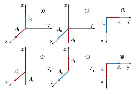
Then, we give the details of the local unitary transformations and degeneracy. According to their relationship between the Bloch vectors of and the z axis, there are six cases of the observers in ICHSH2I_{CHSH}^{2}, as shown in Fig. 1. Only the measurement directions (up to rotations about the z axis) of AaA_{a} are plotted, since BaB_{a} can be uniquely determined by AaA_{a} when ICHSH2\langle I_{CHSH}^{2}\rangle reaches the maximal violation. These six cases have a two-to-one correspondences with the three possible choices of the NN-qubit operators in Theorem 2 which are (i): ①, ②; (ii): ③, ④; and (iii): ⑤, ⑥.

According to the equivalence relations under the local unitary transformations on the NN-qubit system and the exchange between 𝔸0\mathbb{A}_{0} and 𝔸1\mathbb{A}_{1}, it is sufficient to consider only the degeneracy of ICHSHNI_{CHSH}^{N} corresponding to cases ① and ⑤. For the case ①, there are six types of the unitary operator uu to consider, corresponding to the six cases in Fig. 1 as the final states of AaA_{a}. However, only two types of uu for the case ⑤ need to be considered, corresponding to the final states in ⑤ and ⑥. This is because, it is equivalent to the one in case ①, if the NN-qubit operators ICHSHNI_{CHSH}^{N} can be transformed by j=1Nuj\bigotimes_{j=1}^{N}u_{j} into the cases (i) or (ii) in Theorem 2. As show in Fig. 2, for fixed 𝔸a\mathbb{A}_{a} and uu, one can derive the unitary operators uju_{j} by requiring Γ(j=1N1uj𝔸aj=1N1uj)=uΓ(𝔸a)u\Gamma(\bigotimes_{j=1}^{N-1}u_{j}^{{\dagger}}\mathbb{A}_{a}\bigotimes_{j=1}^{N-1}u_{j})=u^{{\dagger}}\Gamma(\mathbb{A}_{a})u. We remark that, the initial and final directions of two Bloch vectors can uniquely determine a 2×22\times 2 unitary operator, up to a phase factor which does not affect value of ICHSHN\langle I_{CHSH}^{N}\rangle in (27).

j=1N1Xj,j=1N1Xj\bigotimes_{j=1}^{N-1}X_{j},\bigotimes_{j=1}^{N-1}X_{j}^{\prime}j=1N1ujXjuj,j=1N1ujXjuj\bigotimes_{j=1}^{N-1}u_{j}^{\dagger}X_{j}u_{j},\bigotimes_{j=1}^{N-1}u_{j}^{\dagger}X_{j}^{\prime}u_{j}uA0u,uA1uu^{\dagger}A_{0}u,u^{\dagger}A_{1}uA0,A1A_{0},A_{1}j=1N1uj\bigotimes_{j=1}^{N-1}u_{j}Γ\GammaΓ\Gammauu
Figure 2: Procedure to determine the requirements for uju_{j}, XjX_{j} and XjX_{j}^{\prime}.

Case ①.– The case ① exists only in the system with an even NN. The angles φj\varphi_{j}^{\prime} in 𝔸1\mathbb{A}_{1} can always be adjusted to zero by local rotations about the z axis, which transforms A1A_{1} into σx\sigma_{x} simultaneously. In addition, the single-qubit operators in 𝔸0\mathbb{A}_{0}, Xj=±σzX_{j}=\pm\sigma_{z} have even minus signs. These minus signs can be removed by qubit flips without affecting the corresponding A0{A}_{0}. Therefore, one can choose the initial observables as

X1==XN1=σz,X1==XN1=σx;A0=σz,A1=σx.X_{1}=...=X_{N-1}=\sigma_{z},\ \ \ X_{1}^{\prime}=...=X_{N-1}^{\prime}=\sigma_{x};\ \ \ {A}_{0}=\sigma_{z},\ \ \ {A}_{1}=\sigma_{x}. (28)

To construct the local unitary transformations uu and uju_{j}, we introduce three sets of unitary operators as

u(1)=𝟙,\displaystyle u^{(1)}=\openone, u(2)=σx,\displaystyle u^{(2)}=\sigma_{x}, u(3)=exp(iσy2π2),\displaystyle u^{(3)}=\exp(i\frac{\sigma_{y}}{2}\frac{\pi}{2}), u(4)=σzu(3),\displaystyle u^{(4)}=\sigma_{z}u^{(3)}, u(5)=exp(iσx2π2),\displaystyle u^{(5)}=\exp(-i\frac{\sigma_{x}}{2}\frac{\pi}{2}), u(6)=σxu(5);\displaystyle\!\!\!\!\!\!\!\!\!u^{(6)}=\sigma_{x}u^{(5)}; (29a)
v(1)=u(1),\displaystyle v^{(1)}=u^{(1)}, v(2)=u(2),\displaystyle v^{(2)}=u^{(2)}, v(3)=u(3),\displaystyle v^{(3)}=u^{(3)}, v(4)=u(4),\displaystyle v^{(4)}=u^{(4)}, v(5,6)={u(5,6)N/2 is even,u(6,5)N/2 is odd;\displaystyle v^{(5,6)}=\begin{cases}u^{(5,6)}&\text{$N/2$ is even},\\ u^{(6,5)}&\text{$N/2$ is odd};\end{cases}\!\!\!\!\!\!\!\!\! (29b)
w(1)=σxv(1),\displaystyle w^{(1)}=\sigma_{x}v^{(1)}, w(2)=σxv(2),\displaystyle w^{(2)}=\sigma_{x}v^{(2)}, w(3)=σzv(3),\displaystyle w^{(3)}=\sigma_{z}v^{(3)}, w(4)=σzv(4),\displaystyle w^{(4)}=\sigma_{z}v^{(4)}, w(5)=σxv(5),\displaystyle w^{(5)}=\sigma_{x}v^{(5)}, w(6)=σxv(6).\displaystyle\!\!\!\!\!\!\!\!\!w^{(6)}=\sigma_{x}v^{(6)}. (29c)

For an arbitrary superscript ν=1,,6\nu=1,...,6, one can check the NN-qubit GHZ state has a symmetry as

v(ν)N1u(ν)|G=exp(iϕ)|G,{v^{(\nu)}}^{\otimes N-1}{u^{(\nu)}}^{*}|G\rangle=\exp(i\phi)|G\rangle, (30)

where v(ν)N1{v^{(\nu)}}^{\otimes N-1} denotes the direct product of N1N-1 v(ν)v^{(\nu)} on the first N1N-1 qubits and ϕ[0,2π]\phi\in[0,2\pi] is a phase factor. This can be regarded as an extension of the symmetry of the Bell state in (26).

The operator uu, transforming the initial AaA_{a} into the case $\nu$⃝, can be universally written as

u=u(ν)exp(iσz2δ)u=u^{(\nu)}\exp(i\frac{\sigma_{z}}{2}\delta) (31)

with δ[0,2π]\delta\in[0,2\pi]. According to the correspondences between the six cases and the three possible choices in Theorem 2, there are two alternative forms of uju_{j} as

uj=v(ν)exp(iσz2δj)orw(ν)exp(iσz2δj),u_{j}=v^{(\nu)}\exp(i\frac{\sigma_{z}}{2}\delta_{j})\ \ \ \text{or}\ \ \ w^{(\nu)}\exp(i\frac{\sigma_{z}}{2}\delta_{j}), (32)

with j=1,,N1j=1,...,N-1 and δj[0,2π]\delta_{j}\in[0,2\pi]. Applying them onto AaA_{a} and 𝔸a\mathbb{A}_{a} and requiring Γ(j=1N1uj𝔸aj=1N1uj)=uΓ(𝔸a)u\Gamma(\bigotimes_{j=1}^{N-1}u_{j}^{{\dagger}}\mathbb{A}_{a}\bigotimes_{j=1}^{N-1}u_{j})=u^{{\dagger}}\Gamma(\mathbb{A}_{a})u, one can easily obtain the two conditions on uju_{j}, as

j=1N1δj=δmod2π,\sum_{j=1}^{N-1}\delta_{j}=\delta\mod 2\pi, (33)

and the number of w(ν)w^{(\nu)} in j=1N1uj\bigotimes_{j=1}^{N-1}u_{j} being even.

Then, j=1Nuj|G\bigotimes_{j=1}^{N}u_{j}|G\rangle are eigenstates of the inital ICHSHNI^{N}_{CHSH}, with the same eigenvalue as |G|G\rangle. By utilizing the forms of uju_{j} in (32) and uN=uu_{N}=u^{*} in (31), one can derive these states in three steps : (1) rotations about the z axis with exp(iσz2δj)\exp(i\frac{\sigma_{z}}{2}\delta_{j}) and exp(iσz2δ)\exp(-i\frac{\sigma_{z}}{2}\delta); (2) v(ν)v^{(\nu)}, including the ones in w(ν)w^{(\nu)}, and u(ν){u^{(\nu)}}^{*}; (3) the even number of σx\sigma_{x} or σz\sigma_{z} factored out from w(ν)w^{(\nu)}. The state |G|G\rangle is invariant under the operations in the first two steps, because of the condition (33) and the symmetry (30). Consequently, j=1Nuj|G\bigotimes_{j=1}^{N}u_{j}|G\rangle are equivalent to the results of |G|G\rangle multiplied by even number of σx\sigma_{x} or σz\sigma_{z}. Since |G|G\rangle is invariant under even number of σz\sigma_{z}, the degenerate states are given by qubit flips in pairs (i.e., application of even number of σx\sigma_{x}) on |G|G\rangle. The degeneracy can be directly derived as

CN10+CN12++CN1N2=2N2.C_{N-1}^{0}+C_{N-1}^{2}+...+C_{N-1}^{N-2}=2^{N-2}. (34)

Case ⑤.– One can always adjust the angles φj\varphi_{j} in 𝔸0\mathbb{A}_{0} to zero by using local rotations about the z axis, which transform A0A_{0} into σx\sigma_{x} and A1A_{1} into σy\sigma_{y} simultaneously. Then, the initial observables can be choose as

Xj=σx,Xj=cosφjσx+sinφjσy;A0=σx,A1=σy,X_{j}=\sigma_{x},\ \ \ X_{j}^{\prime}=\cos\varphi_{j}^{\prime}\sigma_{x}+\sin\varphi_{j}^{\prime}\sigma_{y};\ \ \ {A}_{0}=\sigma_{x},\ \ \ {A}_{1}=\sigma_{y}, (35)

with j=1,,N1j=1,...,N-1 and j=1N1φj=π/2mod2π\sum_{j=1}^{N-1}\varphi_{j}^{\prime}=\pi/2\mod 2\pi.

In order to express in a similar way as the case ①, we define

u(5)=𝟙,\displaystyle u^{(5)}=\openone, v(5)=u(5),\displaystyle v^{(5)}=u^{(5)}, w(5)=σxu(5);\displaystyle w^{(5)}=\sigma_{x}u^{(5)}; (36a)
u(6)=σx,\displaystyle u^{(6)}=\sigma_{x}, v(6)=u(6),\displaystyle v^{(6)}=u^{(6)}, w(6)=σxu(6).\displaystyle w^{(6)}=\sigma_{x}u^{(6)}. (36b)

Similarly, the NN-qubit GHZ state has a symmetry as

v(μ)N1u(μ)|G=exp(iθ)|G,{v^{(\mu)}}^{\otimes N-1}{u^{(\mu)}}^{*}|G\rangle=\exp(i\theta)|G\rangle, (37)

with μ=5,6\mu=5,6 and θ[0,2π]\theta\in[0,2\pi] being a phase factor. The operators transforming the initial AaA_{a} and 𝔸a\mathbb{A}_{a} into the case $\mu$⃝, can be written as

u=u(μ)exp(iσz2δ),\displaystyle u=u^{(\mu)}\exp(i\frac{\sigma_{z}}{2}\delta), (38)
uj=v(μ)exp(iσz2δj)orw(μ)exp(iσz2δj),\displaystyle u_{j}=v^{(\mu)}\exp(i\frac{\sigma_{z}}{2}\delta_{j})\ \ \ \text{or}\ \ \ w^{(\mu)}\exp(i\frac{\sigma_{z}}{2}\delta_{j}), (39)

with δ,δj[0,2π]\delta,\delta_{j}\in[0,2\pi] and j=1,,N1j=1,...,N-1.

We define the sets J={1,2,3,4,N1}J=\{1,2,3,4\cdots,N-1\}, KK and LL, with KJK\subseteq J and LL being its complementary set. The elements of KK are the subscripts of uju_{j} with w(μ)w^{(\mu)}, and ones of LL are for v(μ)v^{(\mu)}. Applying the operators (38) onto AaA_{a} and 𝔸a\mathbb{A}_{a} and requiring Γ(j=1N1uj𝔸aj=1N1uj)=uΓ(𝔸a)u\Gamma(\bigotimes_{j=1}^{N-1}u_{j}^{{\dagger}}\mathbb{A}_{a}\bigotimes_{j=1}^{N-1}u_{j})=u^{{\dagger}}\Gamma(\mathbb{A}_{a})u, one can easily obtain

j=1N1δj=δmod2π,\sum_{j=1}^{N-1}\delta_{j}=\delta\mod 2\pi, (40)

and

kKφj=0modπ.\sum_{k\in K}\varphi_{j}^{\prime}=0\mod\pi. (41)

The latter condition is on the initial observables XjX_{j}^{\prime}, which is a difference with the case ①. The states j=1Nuj|G\bigotimes_{j=1}^{N}u_{j}|G\rangle can be derived by following the same three steps in the case ①, which lead to

j=1Nuj|G=kKσxk|G,\bigotimes_{j=1}^{N}u_{j}|G\rangle=\bigotimes_{k\in K}\sigma_{x}^{k}|G\rangle, (42)

with σxk\sigma_{x}^{k} being the Pauli operator σx\sigma_{x} of the kk-th qubit.

For a fixed KK, kKσxk|G\bigotimes_{k\in K}\sigma_{x}^{k}|G\rangle reaches the maximal violations, only when the initial ICHSHNI^{N}_{CHSH} satisfies the condition (41). Therefore, the number of KK, with which the condition (41) is satisfied, gives the degeneracy of the largest eigenvalue of ICHSHNI^{N}_{CHSH}. Then, the maximum degeneracy in the case ⑤ is 2N22^{N-2}, which can be obtained based on the following facts. The condition (41) cannot be fulfilled simultaneously by a subset of JJ and its complementary set, which sets 2N22^{N-2} as the upper limit on the degeneracy. A simple construction to reach the upper limit is that, φ1==φN2=0\varphi_{1}^{\prime}=...=\varphi_{N-2}^{\prime}=0 and φN1=π/2\varphi_{N-1}^{\prime}=\pi/2.

Example.– An arbitrary choice of the operators 𝔸a\mathbb{A}_{a} and 𝔹a\mathbb{B}_{a} reaching the maximal violation of |G|G\rangle can always be transformed into the above two cases by local unitary operations. The degenerate subspace can also be derived by the same local unitary operations on the above results. We show these by using the example with N=4N=4 provided in Ref. Fan et al. (2021), which belongs to the case ⑤.

The parameters of the observables XjX_{j} and XjX_{j}^{\prime} are given by φ1=φ2=φ4=0,φ1=φ2=φ4=π2\varphi_{1}=\varphi_{2}=\varphi_{4}^{\prime}=0,\varphi_{1}^{\prime}=\varphi_{2}^{\prime}=\varphi_{4}=\frac{\pi}{2}, φ3=π4\varphi_{3}=-\frac{\pi}{4} and φ3=π4\varphi_{3}^{\prime}=\frac{\pi}{4}. Then, ICHSHN=ICHSH2=22\langle I_{CHSH}^{N}\rangle=\langle I_{CHSH}^{2}\rangle=2\sqrt{2}. The operators can be adjusted into the simple form (35) by using τ3=exp(iσz2π4)\tau_{3}=\exp(i\frac{\sigma_{z}}{2}\frac{\pi}{4}) and τ4=exp(iσz2π4)\tau_{4}=\exp(-i\frac{\sigma_{z}}{2}\frac{\pi}{4}) on the third and forth qubits. These lead to φ30\varphi_{3}\rightarrow 0, φ4π/4\varphi_{4}\rightarrow\pi/4, φ3π/2\varphi_{3}^{\prime}\rightarrow\pi/2 and φ4π/4\varphi_{4}^{\prime}\rightarrow-\pi/4. Then, the subsets of JJ, with which the condition (41) are fulfilled, are given by

K=,{1,2},{1,3},{2,3}.K=\emptyset,\ \ \ \{1,2\},\ \ \ \{1,3\},\ \ \ \{2,3\}. (43)

Applying τ3\tau_{3} and τ4\tau_{4} onto kKσxk|G\bigotimes_{k\in K}\sigma_{x}^{k}|G\rangle, one obtains the four degenerate states as

12(|0000+|1111),12(|1100+|0011)12(eiπ4|1010+eiπ4|0101),12(eiπ4|0110+eiπ4|1001),\displaystyle\begin{split}\frac{1}{\sqrt{2}}(|0000\rangle+|1111\rangle),&\ \ \ \ \ \ \frac{1}{\sqrt{2}}(|1100\rangle+|0011\rangle)\\ \frac{1}{\sqrt{2}}(e^{-i\frac{\pi}{4}}|1010\rangle+e^{i\frac{\pi}{4}}|0101\rangle),&\ \ \ \ \ \ \frac{1}{\sqrt{2}}(e^{-i\frac{\pi}{4}}|0110\rangle+e^{i\frac{\pi}{4}}|1001\rangle),\end{split} (44)

which are the same as the results in Ref. Fan et al. (2021).

IV summary

In summary, we relate the two recent topics in the area of Bell-nonlocality, which are the robust violations of Bells inequality of the GHZ states Fan et al. (2021) and the single-qubit quantum game Henaut et al. (2018). Namely, we present the mapping from the generalized CHSH inequality, to distinguish the GHZ states constructed by Fan et al. Fan et al. (2021) to the CHSH game, and consequently to the single-qubit CHSH* game Henaut et al. (2018). These relationships provide an explanation for the robust violations of the generalized CHSH inequality in NN-qubit systems. The identity transformation in the CHSH* game, corresponds to the symmetry of the two-qubit Bell state, and further leads to the local unitary transformations generating the degenerate subspace of the NN-qubit Bell function. An arbitrary superposition or mixture in the subspace leads to the same expected value of the Bell function, which is the quantum phenomenon of robust violations. Based on the explanation, we exactly prove that the maximal degeneracy is 2N22^{N-2}. It would be interesting to extend the mapping among the systems with different numbers of subsystems to explore more topics in the area of Bell-nonlocality and entanglement, such as the identification of W states.

Acknowledgements.
This work was supported by the NSF of China (Grants No. 11675119 and No. 11575125).

References

  • Schrödinger (1935) E. Schrödinger, Proc. Cambridge Philos. Soc. 31, 555 (1935).
  • Amico et al. (2008) L. Amico, R. Fazio, A. Osterloh, and V. Vedral, Rev. Mod. Phys. 80, 517 (2008).
  • Horodecki et al. (2009) R. Horodecki, P. Horodecki, M. Horodecki, and K. Horodecki, Rev. Mod. Phys. 81, 865 (2009).
  • Hill and Wootters (1997) S. Hill and W. K. Wootters, Phys. Rev. Lett. 78, 5022 (1997).
  • Wootters (1998) W. K. Wootters, Phys. Rev. Lett. 80, 2245 (1998).
  • Torun and Yildiz (2019) G. Torun and A. Yildiz, Phys. Rev. A 100, 022320 (2019).
  • Einstein et al. (1935) A. Einstein, B. Podosky, and N. Rosen, Physical Review 47, 777 (1935).
  • Bell (1964) J. S. Bell, Physics 1, 195 (1964).
  • Das et al. (2017) A. Das, C. Datta, and P. Agrawal, Phys. Lett. A 381, 3928 (2017).
  • Das et al. (2018) A. Das, C. Datta, and P. Agrawal, arXiv: 1809.05727 (2018).
  • Brunner et al. (2014) N. Brunner, D. Cavalcanti, S. Pironio, V. Scarani, and S. Wehner, Rev. Mod. Phys. 86, 419 (2014).
  • Scarani (2019) V. Scarani, Bell Nonlocality (Oxford Univ. Press, 2019).
  • Gisin and Bechmann-Pasquinucci (1998) N. Gisin and H. Bechmann-Pasquinucci, Physics Letters A 246, 1 (1998).
  • Ren et al. (2019) C. Ren, T. Feng, D. Yao, H. Shi, J. Chen, and X. Zhou, Phys. Rev. A 100, 052121 (2019).
  • Reid et al. (2009) M. D. Reid, P. D. Drummond, W. P. Bowen, E. G. Cavalcanti, P. K. Lam, H. A. Bachor, U. L. Andersen, and G. Leuchs, Rev. Mod. Phys. 81, 1727 (2009).
  • Mermin (1990) N. D. Mermin, Phys. Rev. Lett. 65, 1838 (1990).
  • Ardehali (1992) M. Ardehali, Phys. Rev. A 46, 5375 (1992).
  • Clauser et al. (1969) J. F. Clauser, M. A. Horne, A. Shimony, and R. A. Holt, Phys. Rev. Lett 23, 880 (1969).
  • van Dam (2000) W. van Dam, Ph.D. thesis, University of Oxford (2000).
  • Ji et al. (2008) S.-W. Ji, J. Lee, J. Lim, K. Nagata, and H.-W. Lee, Phys. Rev. A 78, 052103 (2008).
  • Henaut et al. (2018) L. Henaut, L. Catani, D. E. Browne, et al., Phys. Rev. A 98, 060302 (2018).
  • Fan et al. (2021) X.-Y. Fan, J. Zhou, H.-X. Meng, C. Wu, A. K. Pati, and J.-L. Chen, Mod. Phys. Lett. A 36, 2150223 (2021).