Robust Tracking and Model Following Controller Based on Higher Order Sliding Mode Control and Observation: With an Application to MagLev System
Abstract
This paper deals with the design of robust tracking and model following (RTMF) controller for linear time-invariant (LTI) systems with uncertainties. The controller is based on the second order sliding mode (SOSM) algorithm (super twisting) which is the most effective and popular in the family of higher order sliding modes (HOSM). The use of super twisting algorithm (STA) eliminates the chattering problem encountered in traditional sliding mode control while retaining its robustness properties. The proposed robust tracking controller can guarantee the asymptotic stability of tracking error in the presence of time varying uncertain parameter and exogenous disturbances. Finally, this strategy is implemented on a magnetic levitation system (MagLev) which is inherently unstable and nonlinear. While implementing this proposed RTMF controller for MagLev system, a super twisting observer (STO) is used to estimate the unknown state i.e the velocity of the ball which is not directly available for measurement. It has been observed that the RTMF controller based on STA-STO pair, is not good enough to achieve SOSM for a chosen sliding surface using continuous control. As a remedy, continuous RTMF controller based on STA is implemented with a higher order sliding mode observer (HOSMO). The simulated as well as the experimental results are provided to illustrate the effectiveness of the proposed controller-observers pair.
Index Terms:
Sliding mode control, Super-twisting control, Higher order sliding mode observerI Introduction
The main task in the design of a model following controller is to come up with a control algorithm which compels the dynamics of a specified plant to follow the model dynamics. The tracking error between the model and plant outputs should asymptotically converge to zero making sure that the plant outputs follow the model output perfectly. This approach has the complete freedom to specify all the design criteria through model to ensure the minimization of error between model and plant output [1]–[2].
In the model based control strategy the mismatch between the model of the plant and the actual plant dynamics exists due to the presence of external disturbances, parametric uncertainties and unmodeled dynamics resulting in declination of performance of the closed loop system. This necessitates the design of various robust controllers. Therefore, the problem of RTMF for a class of dynamical system has gathered good amount of attention amongst many researchers in the recent past [3]–[14].
In [3], a nonlinear control scheme is proposed to achieve robust tracking of dynamical signals. Linear state feedback controller is developed for robust tracking and model following of uncertain linear system in [4]. In [5], the problem of RTMF is considered for a class of dynamical systems which contain uncertain nonlinear terms and bounded unknown disturbances. However, these robust state feedback tracking controllers do not produce asymptotic tracking; instead, the so-called practical tracking is achieved.
Sliding mode control (SMC) technique has been recognized as one of the efficient tools to design robust controller for systems operating under various uncertainty conditions [1], [15]–[17]. It has many attractive features such as insensitive to matched uncertainties, order reduction, invariance and simplicity in design. The two step design procedure of sliding mode controller consists of design of a sliding manifold which reflects the desired performance during sliding and a discontinuous control law which makes sure that the state trajectories evolving in the sliding manifold [1] stays there for all future time. Based on SMC theory, a class of variable structure tracking controllers has been proposed in [6]–[14] for robust tracking and model following of dynamical signals for a class of uncertain dynamical systems. The main disadvantage of these SMC based strategies are the so called “chattering effect” which affects the actuator performance in practical implementation [15]–[17]. Moreover, most of these works in [6]–[14] have been tested only in simulation and no hardware implementation has been found so far in any literature.
In contrast to that, the controller based on STA is the most suitable choice to eliminate chattering due to continuous nature of control signal [17], [18]. It achieves finite-time convergence of not only the sliding variable but its first derivative as well. In the family of HOSM, the most effective SOSM algorithm is the STA because same algorithm can be used as controller [19], observer known as STO [20], [21] and robust exact differentiator [22]. Controller based on STA generates continuous control signal and consequently compensates chattering which ensures all the properties of first order SMC in addition to that it achieves second order sliding motion (SOSM) in the presence of bounded uncertainties.
With this motivation this paper presents a new class of RTMF controllers based on STA and then the proposed control algorithm is implemented in magnetic levitation (MagLev) apparatus (Feedback Instruments Ltd. UK, Model No. 33-210).
Industrial application of MagLev continues to grow world wide and successfully implemented for many applications like high-speed MagLev passenger trains, frictionless bearing, superconductor rotor suspension of gyroscopes, rocket-guiding projects and vibration isolation systems in semiconductor manufacturing. The position control of the levitated ball is a challenging control problem due to the fact that the system is inherently nonlinear and open loop unstable. In past many advanced controllers like robust sliding mode control [23]–[28], feedback linearization based control strategy [29]–[31], PID control [32]–[34], adaptive control [35]–[37], generalised proportional integral (GPI) control [38]–[39] have been proposed for compensation of magnetic levitation system.
The implementation of the proposed RTMF controller based on STA in MagLev system requires the information of position and velocity of the ball, but direct measurement of ball velocity is not available. For estimation of velocity, the measured position data is numerically differentiated in most of the literature dealing with control law implementation for MagLev system. This process is not suitable from the implementation point of view because differentiation will enhance the high frequency noise in the position measurement. In [29], a nonlinear observer with linear error dynamics is designed to estimate the speed. An model based integral re-constructor is proposed in [39] for online ball velocity estimation. However, these methodologies suffer from a drawback is that the estimators are not robust against the uncertainties. This fact was the motivation to design STO which is insensitive with respect to uncertainties to estimate the ball velocity of MagLev which is complemented with proposed RTMF controller based on STA. But it has been observed that with this RTMF controller based on STA with STO it is not possible to achieve SOSM using continuous control. As a remedy, continuous RTMF controller based on STA is implemented with a HOSMO. With this observation it can be said that the performance of RTMF based on STA with STO as well as with HOSMO has been validated experimentally first time with magnetic levitation apparatus.
The contribution can be summarized as follows:
-
•
The design of RTMF based on STA is proposed for a class of uncertain LTI systems which will generate continuous control signal, and consequently suppress the effect of chattering.
-
•
To validate the performance of this proposed controller, the implementation is done in MagLev system.
-
•
To avoid the implementation difficulties, the velocity of the levitated ball is estimated using STO and the RTMF based on STA is designed and implemented based on this estimated velocity. With this method it is not possible to achieve continuous control for chosen sliding surface. As a remedy, continuous RTMF controller based on STA is implemented with a HOSMO.
The rest of the paper is organized as follows. Section 2 gives some preliminaries and problem statement. Section 3 presents the design steps of RTMF controller based on STA for an uncertain LTI system. In section 4 dynamic model of the MagLev system is derived. In selection 5 the selection of model is discussed along with the design of RTMF controller based on STO and HOSMO for MagLev. In section 6 both simulated and experimental results are presented. Finally, Section 7 concludes the paper.
II Problem formulation and assumption
Consider a order linear time invariant (LTI) uncertain dynamical system as
| (1) | ||||
| (2) |
where is the state vector, the control input is given by the mapping which is Lebesgue measureable, is the output vector which is to track the reference input and are constant real matrices. The matrix is known and the function is unknown exogenous input. Throughout the paper the following assumptions hold.
Assumption 1
The pair is completely controllable.
Assumption 2
The parametric uncertainties viz., , , and the exogenous input signal are Lipschitz continuous in their arguments. This is indeed necessary to ensure uniqueness of system trajectory.
Assumption 3
Any uncertainties and disturbances entering into the system satisfy the matching condition, i.e., all uncertain quantities reside in range space of , . Therefore, there exist matrices , and such that
From the structural assumption all uncertainties can be lumped and the system (II) can be rewritten as
| (3) | ||||
where, is a lumped uncertain vector.
Assumption 4
i.e continuously differentiable in and piecewise continuous in . Then there exists a positive constant such that
| (4) |
In this paper the objective is to design the control law to make the output of the system (3) to follow the output of the reference model. Consider the reference model is given by
| (5) | ||||
where is the state vector of the reference model, has the same dimension as and are constant matrices of appropriate dimensions. The reference input is assumed to be the output of the model. Further, it is assumed that the model states are bounded, i.e., there exists a finite positive constant such that , . The reference model represents the ideal response that the controlled system must follow.
It has been shown in [4] that if there exist matrices and such that the following matrix algebraic relation holds
| (12) |
then the RTMF control based on STA proposed latter in (40) will ensure that the output of the system (3) will follow the output of (5). If a solution to (12) is not found, then a different reference model must be chosen. A method of solution to (12) is discussed in [4] which is revisited in the following discussion briefly. To solve (12), it is assumed that
This condition is satisfied if the nominal system is controllable and the number of outputs is less than or equal to the number of inputs, i.e., . If this satisfy, then solution to (12) can be written as
| (19) | ||||
| (24) | ||||
| (29) |
where is an matrix, is an matrix, is an matrix, and is an matrix. Specifically, if then :
| (32) |
and is partitioned accordingly in the same way. An equivalent form of (19) is
| (33) |
| (34) |
The above relations can be solved simultaneously for and . Though there are many methods exist to solve for the above relation here we discuss the method given in [4]. Let be any matrix
where denotes the row of . We define a stacking operator for the matrix as
| (35) |
The vector is obtained by stacking the transpose of the rows of . To solve (33), we write it as
| (36) |
This equation can be solved using the Kronecker product . The Kronecker product of two matrices and is defined as
| (37) |
The resultant matrix is of the order . Using the stacking operator and the Kronecker product, (36) reduces to
| (38) |
which is a system of linear equations for components of . Then is found by unstacking . Once is solved, substituting for into (34) yields .
III Design of robust tracking controller
Our design objective can be stated as: given a desired model and its output, find a RTMF controller to force the uncertain system under consideration to behave as the ideal model, i.e., have the same or similar rise time, settling time, damping, etc. To achieve this, we propose a RTMF controller based on STA which can guarantee the output of uncertain system (3) will follow the output of reference model (5) ensuring asymptotic convergence of tracking error to zero. Let the tracking error be defined as
| (39) |
Then the tracking control law is proposed as
| (40) |
where is a super twisting control law. A new auxiliary state vector is defined as follows
| (41) |
Using (12) and (41), the relation between tracking error and new state vector can be written as
| (42) |
From (42), we can see that , and as , it’s evident that . So, it’s enough to only think about stability of . From (5), (40) and (41), the auxiliary system can be expressed as
| (43) |
A convenient way to solve this problem is to first transform the system (43) into a suitable canonical form. In order that, partition (43) as
where and , and . Define the following orthogonal transformation
| (46) |
where is a indentity matrix, now define the new coordinate of transformation as
| (49) |
Therefore, (43) can be written with the help of above transformation in the regular form as
| (60) |
where and . In order to achieve robustness against matched uncertainty, we design STA for the (60). Since STA is a first order control algorithm, so a hypersurface is designed such that the control appears in its first derivative. This technique achieves asymptotic stability of the system once this hypersurface is reached in finite time.
We define the sliding variable as
| (64) |
where is chosen by some appropriate design procedure and . Further, define a linear change of coordinates by
If this transformation represents the new coordinates as
then dynamics in the new coordinates is
| (73) |
where
Design the control input as
| (78) |
Substituting the control input in (73) the system equation becomes
| (87) | ||||
| (90) |
where the components of are
| (91) | ||||
where are the scalar gains. Let and substituting (91) in (87) then the closed loop system
| (92) | ||||
| (93) | ||||
| (94) |
where the vector with each component for and . The closed loop dynamics (92)–(94) consist of a set of differential inclusion and the solution to this are understood in sense of Filippov [40].
Theorem 1
To show (95) and (96) finite time stable, the Lyapunov function can be chosen as where , then the trajectories of the system (95)-(96) will converge to origin in a finite time smaller than [41]
where
for positive and symmetric definite matrices and . Here the gains for can be selected to achieve and zero in some finite time.
Select the gains and as and . The gains and are enough to bring in finite time. Hence from (92), the reduced order dynamics or zero dynamics of the system with respect to becomes
| (97) |
The pair is controllable pair and can be designed in such way that i.e (97) becomes globally asymptotically stable. This ends the proof.
Proposition 1
Proof : From Theorem 1, it is shown that the sliding surface goes to zero in finite time. Using (97), it can be concluded that
| (98) | ||||
Now using (64) and (98), it yields
| (99) |
Then, it follows immediately from (49), (98) and (99) that
| (100) |
Recalling relationship between and , i.e. , we obtain that the tracking error also decreases asymptotically to zero.
The real time implementation of the proposed control law for magnetic levitation system is developed in the following sections.
IV Dynamical Model of the MagLev system
A simplified schematic diagram of the MagLev system is shown in Fig.1. The system is mainly computer controlled and user’s specific control law can be implemented and applied on the system in realtime using MATLAB/SIMULINK environment
through a PCI 1711 AD card.
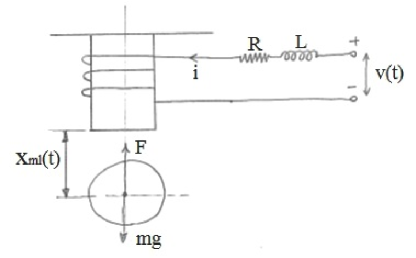
Our main task here is vertical position control of the levitated ball by application of a suitable current i(t) by means of applying a voltage v(t) in the coil. R and L represents the resistance and inductance of the coil, respectively. Here denotes the distance by which the coil magnet and the ball’s center are separated. The nonlinear force applied by the magnet is , where is a positive constant. The differential equation capturing dynamics of the system is of the form
| (101) | ||||
| (102) |
where denotes mass of the levitated ferromagnetic ball, is the gravitational acceleration and is a proportionality constant [42] which depends upon the input voltage and coil current. To design the proposed robust model following controller, the model is linearized around an equilibrium point and the transfer function of the system is found as
| (103) |
where , . The ball position is measured by the IR sensor in voltage and they are linearly related with a proportionality constant . Finally with , the above transfer function can be rewritten as
| (104) |
The nominal system parameters are shown in Table I. From the open loop transfer function it is clear that the system is severely unstable.
In state space representation (104) can be written as
| (105) | ||||
From (105), it is clear that the MagLev is a second order electro-mechanical system whose relative degree is two [43].
| Parameter | Value |
|---|---|
| Kg | |
| m/ | |
| A | |
| m | |
| A/V | |
| V/m | |
| V | |
| V to V |
V Design of the proposed controller for MagLev system
In this section the proposed robust tracking and model following control strategy is designed for the MagLev system which is affected by model uncertainties and external disturbances, then (105) can be rewritten as
| (110) | ||||
| (112) |
where the lumped disturbance applied to the plant is chosen as .
The task of the robust model following controller is to ensure the asymptotic convergence of tracking error between model and the plant output to zero. The essential part for the controller design is to select a suitable model which the plant needs to follow. The selection of a suitable model for the MagLev system is discussed in the following subsection.
V-A Selection of the Model
Proportional-integral-derivative (PID) controller is widely used for the effective regulation of the real systems without uncertainty. In this work, the nominal MagLev system with PID controller is used to find a suitable model. With PID controller and the open loop transfer function of MagLev , where , , the closed loop transfer function is computed as follows
| (113) |
The values of the controller gains are selected such that the closed loop poles are located at [39]. With these gains, (V-A) can be represented as follows
| (114) | ||||
| (115) |
where
and
Now from (12), and matrices can be easily computed with the knowledge of the system and model matrices which is shown below
| (118) | ||||
| (120) |
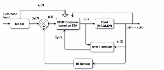
To apply the proposed RTMF controller based on STA on MagLev which is a second order electromechanical system with relative degree two to compensate the chattering problem, the design of sliding surface (64) will be such that it’s relative degree must be one. In that situation we require the information of two states i.e. ball position and ball velocity of MagLev system. In practice only ball position is available for measurement. In the following section it has been shown that using STO it is possible to estimate the ball velocity in finite time in the presence of uncertainties and using this estimated information, the proposed RTMF controller based on STA is possible to design. The block diagram of this proposed scheme is shown in Fig. 2.
V-B Design of Proposed RTMF Controller based on STO
To design the STO to estimate the states of MagLev system (110), let us rewrite the plant dynamics (110)
| (121) | ||||
The STO dynamics can be written as
| (122) | ||||
| (123) |
Where and are the estimation errors. Then the error dynamics can be written as
| (124) | ||||
| (125) |
From Assumption 4, . In [41], [44] the finite time stability of the above error dynamics has been established with the choice of and . This ensures the finite time convergence of estimation errors and to zero which essentially leads to and in finite time.
To design the proposed RTMF controller, system is required to transform in coordinate using (41). Using the relation for MagLev system following can be written
| (126) |
Where and are the states of the chosen model (114) and is the estimated ball velocity by STO. Using (110), (118), (123) and (126) the derivative of and can be written as
| (127) | ||||
| (128) |
Now choosing a sliding manifold of the following form
| (129) |
and differentiating (129), the sliding dynamics can be written as
| (130) |
Now using (127) and (128), we can write (130) as
| (131) |
Using (120), the proposed control law (40) can be written as
| (136) |
Now using (136), replacing , and choosing we can write (131) as
| (137) |
Now choosing the control input as
| (138) |
where and are controller design parameters, (137) can be written as
| (139) |
Using the fact , (129) and (139), the closed loop system can be represented in ( , ) coordinate as follows
So the overall closed loop system with controller-observer together now can be represented as
| (140) |
The observer error for the system goes to zero in finite time. In [45] it has been established that, the trajectories of the system cannot escape in finite time. Generally, observer gains are chosen in such a way that the estimation error converges faster. This fact allows to design the observer and the control law separately, i.e., the separation principle is satisfied. With , the closed-loop system can be written as
| (141) | ||||
From the last two equations of (141) it is evident that it has the same structure as STA. So it is easy to conclude that in finite time , then the reduced order system dynamics can be represented as
Therefore both states and are asymptotically stable and using Proposition 1 it can be said that the tracking error also converges to zero asymptotically.
Remark 1
The additional term is added in (138) because in [21] it has been shown that it is not possible to achieve the continious control when super twisting controller is implemented with STO. To solve this implementation issues, a continuous RTMF controller based on STA is proposed with higher order sliding mode observer (HOSMO) like in [21] that achieves the second order sliding mode.
V-C Design of Proposed RTMF Controller based on HOSMO
To estimate the velocity of the uncertain MagLev system (110), the dynamics of HOSMO [21] is presented as
| (142) |
where and are the estimation error variables. The error dynamics can be written as
| (143) | ||||
By means of transformation and with the assumption 4, the system (143)can be written as
| (144) | ||||
In [46], it has been already proved that the (144) is finite time stable and by selecting the appropriate gains , and it can be guaranteed that , and will converge to zero in finite time [47].
Now, the design of RTMF based on STA can be formulated with the estimated velocity . Using relation Using (110), (118), (126) and (142) we have
| (145) | ||||
| (146) |
Now choosing a sliding surface same as (129)
| (147) |
Taking derivative of (147) and using (145) and (146) we get
| (148) |
Now using (137) and choosing we can write (148) as
| (149) |
Now choosing as
| (150) |
Where and are controller design parameters, then we can write (149) as
| (151) |
Now using the fact , (147) and (151) the closed loop system can be represented in coordinates as follows
| (152) |
So the overall closed loop dynamics with controller-observer together can be represented as
| (153) |
It has been already discussed that the observer error for the system goes to zero in finite time. In [45] it has been established that, the trajectories of the system cannot escape in finite time. By substituting , the closed-loop system can be written as
| (154) | ||||
In (154), the lower two equations are of STA and by selecting appropriate gains and it can be ensured that in finite time which helps to represt the reduced order system as follows
| (155) | ||||
| (156) |
Therefore and goes to zero asymptotically which in turn guarantees the asymptotic convergence of output tracking error .
VI Simulation and experimental results
This section provides the experimental results for MagLev system for two cases a) RTMF controller based on STA with STO and b) RTMF controller based on STA with HOSMO. The simulation and experiment with MagLev system has been performed for these two cases. The external disturbance voltage signal is injected externally to perturb the plant. The output tracking performance of MagLev system is presented for sinusoidal and trapezoidal input for both cases which is mentioned above. The initial condition for the model is taken as .
VI-A RTMF controller based on STA with STO
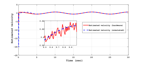
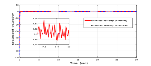
The control strategy based on STO developed in Section 5.2 is implemented for MagLev system. The STO gains are chosen as and and gains of RTMF controller based on STA are chosen as . Fig. 3 and Fig. 4 shows the estimated velocity for the inputs sinusoidal and trapezoidal respectively with STO.
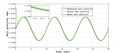
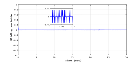
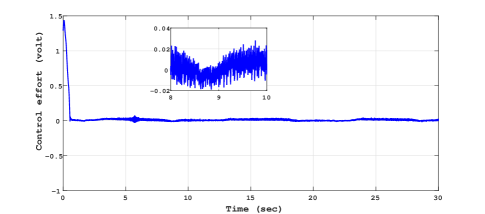
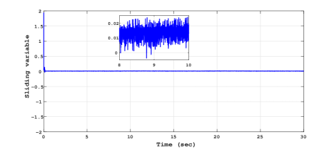
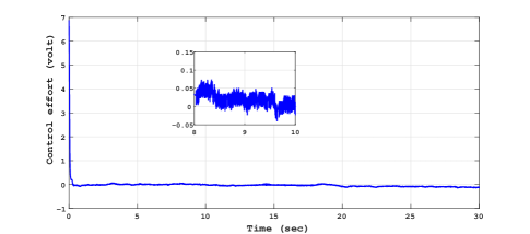
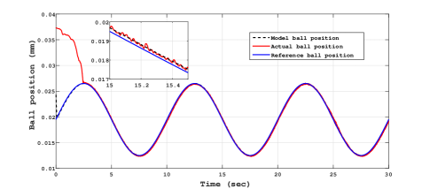
The experimental results for sinusoidal tracking performance, sliding surface and control input is presented in Fig. 5, Fig. 6 and Fig. 7 respectively.
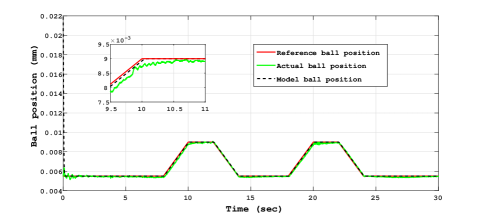
Similarly the experimental results for trapezoidal tracking performance, sliding surface and control input is presented in Fig. 8, Fig. 9 and Fig. 10 respectively.
VI-B RTMF controller based on STA with HOSMO
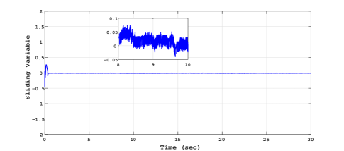
This section is devoted to present the experimental results for the RTMF controller based on STA with HOSMO. To estimate the velocity of the ball of the MagLev system HOSMO is implemented with gains : and . The gains of the RTMF controller based on STA is chosen as . The estimation performance of HOSMO is found similar to STO and the results are not shown because of the space constraint. The experimental results of this controller-observer combination for sinusoidal tracking, sliding surface and control input is presented in Fig. 11, Fig. 12 and Fig. 13 respectively.
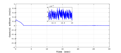
In a similar manner the experimental results for trapezoidal tracking performance, sliding surface and control input is presented in Fig. 14, Fig. 15 and Fig. 16 respectively.
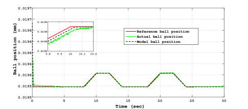
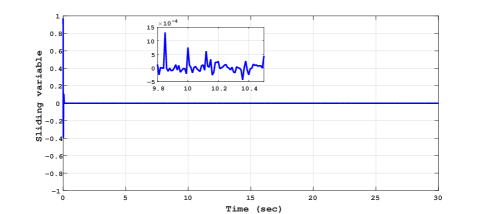
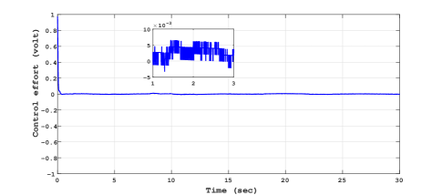
Comparing the control plots Fig. 7, Fig. 10 and Fig. 13, Fig. 16, it is easy to conclude that the control signal is more smoother in case of RTMF controller based on STA with HOSMO compared to RTMF controller based on STA with STO. It is apparent form the sliding surface plots (in zoom plot), the improved precision is achieved in case of RTMF controller based on STA with HOSMO compared to RTMF controller based on STA with STO.
VII Conclusion
In this paper, RTMF controller based on STA is proposed for uncertain LTI systems. To validate the performance of the proposed controller, it is designed and implemented in real time MagLev system in the presence of disturbance. The implementation of this controller for MagLev requires knowledge of both the system states. However only ball position is available for measurement. To avoid the implementation difficulties, the RTMF controller based on STA is designed and implemented with STO. But it has been realized that the continuous control for the chosen sliding surface is not possible to achieve with RTMF controller based on STA with STO. To overcome this issue, a RTMF controller based on STA with HOSMO is designed and implemented for MagLev system. It is clear from the obtained results that the control scheme based on STA provides excellent tracking of time varying signals for both cases during which the system is completely insensitive to disturbances acting on it. It has been also observed that smoother control action with improved precision of sliding variable is achieved in case of RTMF controller based on STA with HOSMO.
References
- [1] C Edwards, S Spurgeon, Sliding Mode Control: Theory And Applications, CRC Press , 1998
- [2] Young, K. -K., “Design of variable structure model-following control systems,” IEEE Transactions on Automatic Control, vol. 23, no. 6, pp. 1079–1085, 1978.
- [3] Corless, M. J., Leitmann,G. and Ryan, E. P., “Tracking in the presence of bounded uncertainties,” 4th International Conference Control Theory, Cambridge, U.K., Sept. 1984.
- [4] Hopp, T. H., and Schmitendorf, W. E., “Design of a linear controller for robust tracking and model following,” ASME Journal of Dynamic Systems, Measurement and Control, vol. 112, pp. 552–558, 1990.
- [5] Sugie, T., and Osuka, K., “Robust model following control with prescribed accuracy for uncertain nonlinear systems,” International Journal of Control, vol. 58, no. 5, pp. 991–1009, 1993.
- [6] J. P. V. S. Cunha, Liu Hsu, R. R. Costa and F. Lizarralde, ”Output-feedback model-reference sliding mode control of uncertain multivariable systems,” IEEE Transactions on Automatic Control, vol. 48, no. 12, pp. 2245-2250, Dec. 2003.
- [7] H. Wu, “Adaptive robust tracking and model following of uncertain dynamical systems with multiple time delays,” IEEE Trans.Automat. Contr, vol. 49(4), pp. 611-616, April. 2004.
- [8] S. K. Spurgeon, C. Edwards and N. P. Foster, “Robust model reference control using a sliding mode controller/observer scheme with application to a helicopter problem,” Proceedings IEEE International Workshop on Variable Structure Systems, Tokyo, Japan, 1996, pp. 36-41.
- [9] Ming Chang Pai, “Design of adaptive sliding mode controller for robust tracking and model following,” Journal of the Franklin Institute, Volume 347, Issue 10, pp. 1837-1849, 2010.
- [10] Wu, H., “Robust tracking and model following for a class of uncertain dynamical systems by variable structure control,” Proceedings of the IEEE International Conference on Control Applications, Anchorage, Alaska, pp. 680–685, 2000.
- [11] S. H. Huh and Z. Bien, “Robust sliding mode control of a robot manipulator based on variable structure-model reference adaptive control approach,” IET Control Theory & Applications, vol. 1, no. 5, pp. 1355-1363, Sept. 2007.
- [12] Kun-Yung Chen, “Model Following Adaptive Sliding Mode Tracking Control Based on a Disturbance Observer for the Mechanical Systems”, J. Dyn. Sys., Meas., Control, vol. 140, no.5, pp. 1–15, 2017.
- [13] I. Tanyer, E. Tatlicioglu, E. Zergeroglu, “Model reference tracking control of an aircraft: a robust adaptive approach”, International Journal of Systems Science, vol. 48, no. 7, pp. 1428–1437, 2017.
- [14] Behrooz Rahmani, “Robust discrete-time sliding mode control for tracking and model following of uncertain nonlinear systems”, International Journal of Systems Science, vol. 49, no. 11, pp. 2427–2441, 2018.
- [15] Utkin, V. I., Sliding Modes in Control and Optimization, Springer-Verlag, 1992.
- [16] Utkin, V. I., Guldner, J. and Shi, J., Sliding Modes in Control in Electro-Mechanical Systems,, Boca Raton, FL: CRC, 2009.
- [17] Shtessel, Y., Edwards, C., Fridman, L., Levant, A., Sliding mode control and observation, Springer, 2014.
- [18] Levant, A., “Sliding order and sliding accuracy in sliding mode control,”, International Journal of Control, vol. 58, no. 6, pp. 1247–1263, 1993.
- [19] Fridman, L., and Levant, A., Sliding Mode Control in Engineering, New York: Marcel Dekker, chap. 3, pp. 53–101, 2002.
- [20] J. Davila, L. Fridman, and L. Arie., “Second-order sliding-mode observer for mechanical systems,” IEEE Trans. Autom. Control, vol. 50, no. 11, pp. 1785–1789, 2005.
- [21] A. Chalanga, S. Kamal, L. M. Fridman, B. Bandyopadhyay and J. A. Moreno, ”Implementation of Super-Twisting Control: Super-Twisting and Higher Order Sliding-Mode Observer-Based Approaches,” IEEE Transactions on Industrial Electronics, vol. 63, no. 6, pp. 3677-3685, June 2016.
- [22] Arie Levant, “Robust exact differentiation via sliding mode technique”, Automatica, 1998, 34, (3), pp. 379–384
- [23] D. Cho, Y. Kato and D. Spilman, “Sliding mode and classical controllers in magnetic levitation systems,” in IEEE Control Systems Magazine, vol. 13, no. 1, pp. 42-48, Feb. 1993.
- [24] H. M. Gutierrez and P. I. Ro, “Magnetic servo levitation by sliding-mode control of nonaffine systems with algebraic input invertibility,” in IEEE Transactions on Industrial Electronics, vol. 52, no. 5, pp. 1449–1455, Oct. 2005.
- [25] H. Chiang, C. Chen and M. Li, “Integral variable-structure grey control for magnetic levitation system,” in IEEE Proceedings - Electric Power Applications, vol. 153, no. 6, pp. 809–814, November 2006.
- [26] F. Lin, S. Chen and K. Shyu, “Robust Dynamic Sliding-Mode Control Using Adaptive RENN for Magnetic Levitation System,” in IEEE Transactions on Neural Networks, vol. 20, no. 6, pp. 938–951, 2009.
- [27] Hsin‐Jang Shieh, Jheng‐Hong Siao, Yu‐Chen Liu, “A robust optimal sliding‐mode control approach for magnetic levitation systems,” in Asian Journal of Control, vol 12, no 4, pp 480–487, 2010.
- [28] P. Roy, S. Sarkar, B. K. Roy and N. Singh, “A comparative study between fractional order SMC and SMC applied to magnetic levitation system,” 2017 Indian Control Conference (ICC), Guwahati, 2017, pp. 473-478.
- [29] W. Barie and J.Chiasson, “ Linear and nonlinear state-space controllers for magnetic levitation”, International Journal of Systems Science, vol 27, no 11, pp 1153–1163, 1996
- [30] Charara, J. De Miras and B. Caron, “Nonlinear control of a magnetic levitation system without premagnetization,” in IEEE Transactions on Control Systems Technology, vol. 4, no. 5, pp. 513-523, Sept. 1996.
- [31] A. El Hajjaji and M. Ouladsine, “Modeling and nonlinear control of magnetic levitation systems,” in IEEE Transactions on Industrial Electronics, vol. 48, no. 4, pp. 831–838, Aug. 2001.
- [32] M. Golob, B. Tovornik, “Modeling and control of the magnetic suspension system”, ISA Transactions, vol. 42, no. 1, pp. 89-100, 2003.
- [33] C. Lin, M. Lin and C. Chen, “SoPC-Based Adaptive PID Control System Design for Magnetic Levitation System,” in IEEE Systems Journal, vol. 5, no. 2, pp. 278-287, June 2011.
- [34] A. Ghosh, T. R. Krishnan, P. Tejaswy, A. Mandal, J. K. Pradhan, S. Ranasingh, “Design and implementation of a 2-DOF PID compensation for magnetic levitation systems”, ISA Transactions, vol. 53, no. 4, pp. 1216–1222, 2014.
- [35] Z. Yang, K. Kunitoshi, S. Kanae and K. Wada, “Adaptive Robust Output-Feedback Control of a Magnetic Levitation System by K-Filter Approach,” in IEEE Transactions on Industrial Electronics, vol. 55, no. 1, pp. 390–399, Jan. 2008.
- [36] F. Lin, L. Teng and P. Shieh, “Intelligent Adaptive Backstepping Control System for Magnetic Levitation Apparatus,” in IEEE Transactions on Magnetics, vol. 43, no. 5, pp. 2009–2018, May 2007.
- [37] P. K. Sinha, A.N. Pechev, “Model reference adaptive control of a maglev system with stable maximum descent criterion,” Automatica, Volume 35, Issue 8, pp. 1457–1465, 1999.
- [38] R. Morales, V. Feliu and H. Sira-Ramirez, ”Nonlinear Control for Magnetic Levitation Systems Based on Fast Online Algebraic Identification of the Input Gain,” in IEEE Transactions on Control Systems Technology, vol. 19, no. 4, pp. 757-771, July 2011.
- [39] R. Morales and H. Sira-Ramírez, “Trajectory tracking for the magnetic ball levitation system via exact feedforward linearisation and GPI control,” International Journal of Control, vol. 83, no. 6, 1155–1166, 2010.
- [40] Filippov, A. F., Differential equations with discontinuous righthand sides, Kluwer academic publiser, Netherlands, 1988.
- [41] Moreno, J. A, and Osorio, M., “Strict Lyapunov functions for the super-twisting algorithm,” IEEE Transactions on Automatic Control, vol. 57, no. 4, pp. 1035–1040, 2012.
- [42] Magnetic Levitation: Control Experiments Feedback Instruments Limited, UK, 2011
- [43] Isidori, A., Nonlinear Control Systems,, third edition, Springer Verlag, Berlin, 1995.
- [44] J. Davila, L. Fridman and A. Levant, ”Second-order sliding-mode observer for mechanical systems,” in IEEE Transactions on Automatic Control, vol. 50, no. 11, pp. 1785-1789, Nov. 2005.
- [45] J. A. Moreno, “A Lyapunov approach to output feedback control using second-order sliding modes”, IMA J. Math Control I., vol. 29, no. 3, pp. 291–308, 2012.
- [46] M. T. Angulo, J. A. Moreno, and L. Fridman, “Robust exact uniformly convergent arbitrary order differentiator,” Automatica, vol. 49, no. 8, pp. 2489–2495, 2013.
- [47] A. Levant, “Higher-order sliding modes, differentiation and output-feedback control,” Int. J. Control, vol. L. 76, no. 9/10, pp. 924–941, 2003.
- [48] S. Ganguly, M. K. Bera and P. Roy, ”Robust Tracking and Model Following Controller based on Sliding Mode: An Experimental Validation with Magnetic Levitation System,” 2019 IEEE 5th International Conference for Convergence in Technology (I2CT), Bombay, India, 2019, pp. 1-6, doi: 10.1109/I2CT45611.2019.9033833.
- [49] S. Ganguly, M. K. Bera and P. Roy, ”Robust Non-overshooting Tracking and Model Following Controller using Multi-variable Super-twisting Algorithm,” 2019 Sixth Indian Control Conference (ICC), Hyderabad, India, 2019, pp. 320-325, doi: 10.1109/ICC47138.2019.9123190.