Robust surface Luttinger surfaces in topological band structures
Abstract
The standard paradigm of topological phases posits that two phases with identical symmetries are separated by a bulk phase transition, while symmetry breaking provides a path in parameter space that allows adiabatic connection between the phases. Typically, if symmetry is broken only at the boundary, topological surface states become gapped, and single-particle surface properties no longer distinguish between the two phases. In this work, we challenge this expectation. We demonstrate that the single-particle surface Green’s function contains zeros, or "Luttinger surfaces," which maintain the same bulk-boundary correspondence as topological surface states. Remarkably, these Luttinger surfaces persist under symmetry-breaking perturbations that destroy the surface states. Moreover, we point out that low-energy and surface theories, often used synonymously in discussions of (gapped) topological matter, are actually different, with the difference captured by the Luttinger surfaces.
Introduction—Bulk-boundary correspondence is a fundamental notion that underpins the standard paradigm of topological band structures. According to this principle, topological materials host robust, gapless surface states that uniquely identify the bulk band topology [1, 2, 3, 4, 5, 6]. In fact, in practice, the surface states invariably serve as the most direct experimental smoking guns of the topological phase. When the bulk undergoes a topological phase transition, the surface also experiences reconstruction, appearance or disappearance of states – in short, a Lifshitz transition [7] – in accordance with the bulk-boundary correspondence. If the topological phase is protected by a symmetry, breaking the symmetry generically destroys the surface states and unlocks a path in parameter space that allows one to adiabatically connect topologically distinct phases. In particular, if the symmetry is broken only on the surface, the bulk topology is well-defined but the surface generically remains gapped along this path. As a result, single-particle physics of the surface is expected to vary smoothly across the bulk phase transition and be qualitatively blind to the bulk topology.
The single-particle Green’s function is a fundamental tool in physics, crucial for characterizing the spectral properties of single-particle excitations as well as describing their response to external perturbations and behavior under interactions and disorder [8, 9]. In Fermi liquids, has poles that directly correspond to the system’s spectrum, with the poles at defining the Fermi surface (FS). In contrast, strongly correlated insulating phases like the Mott insulator have that lacks poles but has zeros within the energy gap. The locus of the zeros of is similarly defined as the Luttinger surface (LS) [10]. Since LSs correspond to the complete absence of quasiparticles, they have traditionally been deemed as peculiar analytic features of indicative of strong correlations, but with little further fundamental or practical value as they are unobservable and do not contribute to physical properties.
Recent breakthroughs, however, have dispelled this notion. Fabrizio proposed a new class of quasiparticles near LSs in strongly correlated systems that produce similar thermodynamic properties as the quasiparticles in a Fermi liquid, such as the linear-in- specific heat [11]. This was followed by several seminal results within the realm of interacting topological condensed matter. Wagner et al. showed that Green’s function zeros characterize the topology of Mott insulators analogous to how poles characterize band insulators [12]. Jinchao et al. [13] and Bollmann et al. [14] discovered that the zeros of the single-particle Green’s function modify the topological invariant, but the latter showed that the zeros do not affect the quantized topological response. Blason and Fabrizio unified the role of poles and zeros in the topological characterization of generic interacting insulators [15]. In contrast to these works, one of us showed that the boundary of a generic Weyl semimetal (WSM) – a non-interacting topological phase – hosts Luttinger arcs in addition to the well-known Fermi arcs [16]. Nonetheless, both structures connect surface projections of Weyl nodes of opposite chirality. All these results place FSs and LSs on similar footing, and are in similar spirit as a pioneering result by Volovik that the same winding number stabilizes FSs and LSs [3].
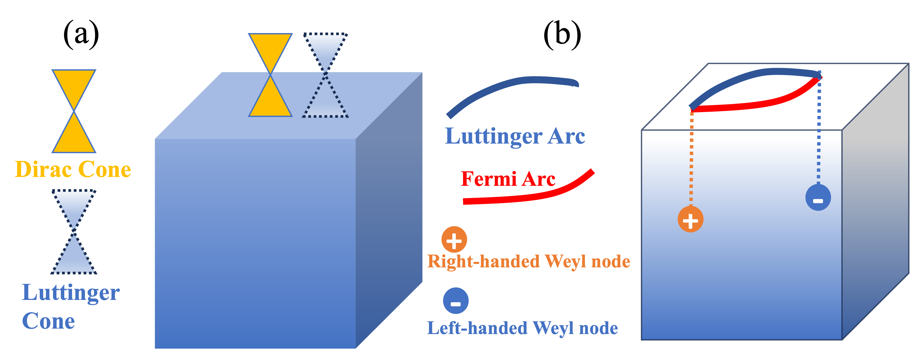
In this work, we begin by proving the existence of surface LSs that respect the same bulk-boundary correspondence as the topological surface states (Fig. 1). As a result, a bulk topological phase would trigger a reconstruction or "Lifshitz transition" of the LSs. We then establish two profound consequences of this behavior. First, we show that surface LSs, remarkably, survive symmetry-breaking perturbations on the surface that destroy the topological surface states. This behavior starkly contradicts the prevailing notion that single-particle boundary properties are oblivious to the bulk topology once the surface states have been gapped out. On the other hand, it is similar in spirit, for instance, to the discontinuity in the surface Hall conductivity of a 3D topological insulator (TI) that is tuned across a bulk topological transition with the surface Dirac node gapped out throughout the process [1, 2]. Second, we show that the LSs reveal a disagreement between two routes for obtaining a low-energy surface theory in topological band structures, leading to unusual thermodynamic properties, such as a negative surface specific heat. We prove all these properties using generic topological arguments and substantiate them numerically using lattice models of 3D time-reversal symmetric TIs and WSMs perturbed by surface magnetism and surface superconductivity, respectively. We close by concretizing the results in the context of Bi2Te3/MnBi2Te4 heterostructures.
Robust surface LSs—We first show that topological band structures not only host surface LSs that obey the same bulk-boundary correspondence as the surface states, generalizing the prediction of surface Luttinger arcs in WSMs [16], but that the LSs have a surprising robustness – they survive even when surface perturbations gap out the surface states.
Consider non-interacting electrons in a -dimensional system with a -dimensional boundary. We label an arbitrary set of degrees of freedom near the boundary as the "surface" and refer to the rest as the "bulk." The full Hamiltonian can be decomposed as
| (1) |
where and are Bloch Hamiltonians for the surface and the bulk, respectively, describe the coupling between them, and is the momentum in the surface Brillouin zone (sBZ). The full and bulk Green’s functions at complex frequency are , , while the effective surface Green’s function obtained by integrating out the bulk degrees of freedom is (see App. A):
| (2) |
The LS is defined as the locus of zero eigenvalues of . To see it emerge, we first note that obeys the condition:
| (3) |
Clearly, every pole of causes to vanish provided stays finite, implying a zero eigenvalue of . Physically, this means surface FSs of that disappear upon coupling and produce surface LSs. At points where and have equal numbers of poles, the situation is subtler. These poles cancel in Eq. 3 and mandate to be finite and non-zero, hence forcing to have equal numbers of diverging (pole) and vanishing (zero) eigenvalues, but does not guarantee the presence of either. On physical grounds, though, we expect surface poles of , i.e., poles whose corresponding eigenstates have finite weight on the surface in the thermodynamic limit, to be inherited by , since they represent physical surface FSs. We prove this explicitly in Appendix B. To ensure a finite , must then also have an equal number of vanishing eigenvalues, thereby defining a LS that coincides with the surface FS. Thus, in all cases, the LS traces the surface FSs of and therefore obeys the same bulk-boundary correspondence as the latter.
This construction instantly yields our first result: LSs persists even when surface FSs are destroyed by symmetry breaking perturbations on the surface. Such perturbations gap out the boundary states of the full system, represented by poles of whose eigenfunctions are localized at the boundary. However, since the bulk degrees of freedom remains unaffected, the poles of persist, and so do the zeros of the . We demonstrate this on a lattice model that realizes 3D TIs and WSMs in next section.
Application to TIs and WSMs—Consider an orthorhombic lattice model defined by the 3D Bloch Hamiltonian [17]:
| (4) |
where , and () are Pauli matrices in orbital (spin) space. The wavevector is defined as . By tuning and , one can induce transitions between a trivial insulator, weak and strong TIs, and WSMs.
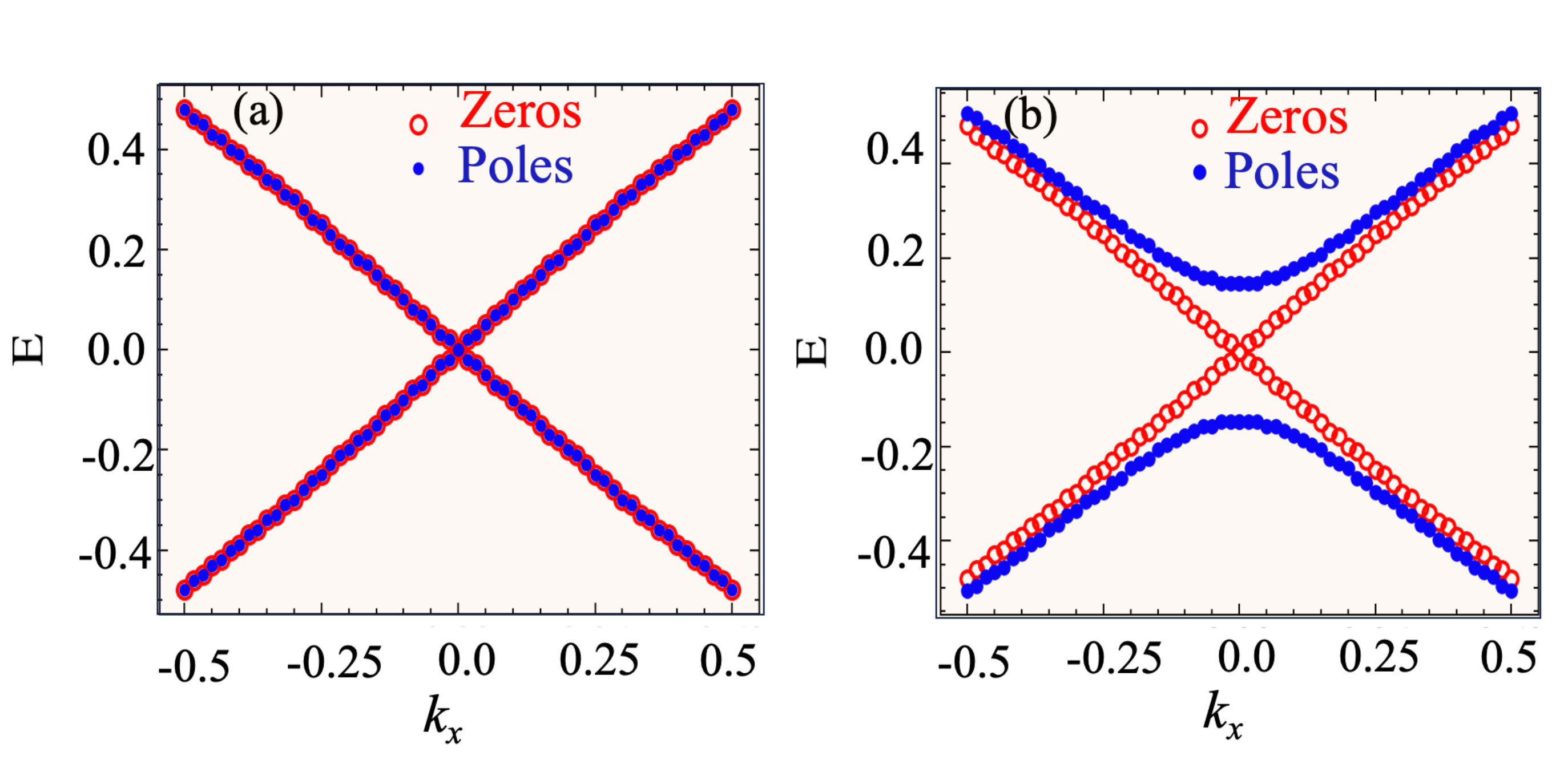
We first consider a strong TI, where we expect a 2D Dirac cone and a 2D Luttinger cone on the surface while time-reversal symmetry is preserved. If the symmetry is broken on the surface, we expect the Dirac cone to disappear but the Luttinger cone to survive. To uncover LSs, we calculate the surface Green’s function [18] recursively (see Appendix E) and locate its zeros (poles) for a given by scanning for values of where the minimum (maximum) singular value of vanishes (diverges) as .
The results are illustrated in Fig. 2 (a) for and agree precisely with this prediction. Clearly, both the poles and zeros form a cone-like dispersion in the sBZ in the absence of the symmetry-breaking surface perturbation. To break the symmetry on the surface, we introduce a surface magnetization , which changes the surface Green’s function to . As shown in Fig. 2(b), the Dirac cone, formed by the poles of , is immediately gapped, but the Luttinger cone, arising from the zeros of , persists. In Appendix C, we further confirm the persistence of the Luttinger cone by calculating the Volovik winding number that endows FSs and LSs with topological stability [3].
As a second test case, we consider WSMs, distinguished by their gapless bulk with chiral topological charges known as Weyl nodes, and surface Fermi arcs connecting the projections of Weyl nodes of opposite chiralities onto the sBZ [19, 4]. The Fermi arcs can also be understood as collections of Bloch momenta on the sBZ where has poles. Similarly, the surfaces of WSMs host Luttinger arcs, defined as regions of the sBZ where has zeros, which cause the non-interacting surface electrons to effectively acquire strong interactions mediated by bulk states [16]. In contrast to the Dirac point on a TI surface, the Fermi arcs cannot be gapped by a simple translationally invariant magnetization perturbation. However, if the WSM is time-reversal symmetric, the Fermi arcs can be gapped by conventional superconductivity, which gives us an opportunity to inspect LSs under another physically relevant perturbation.
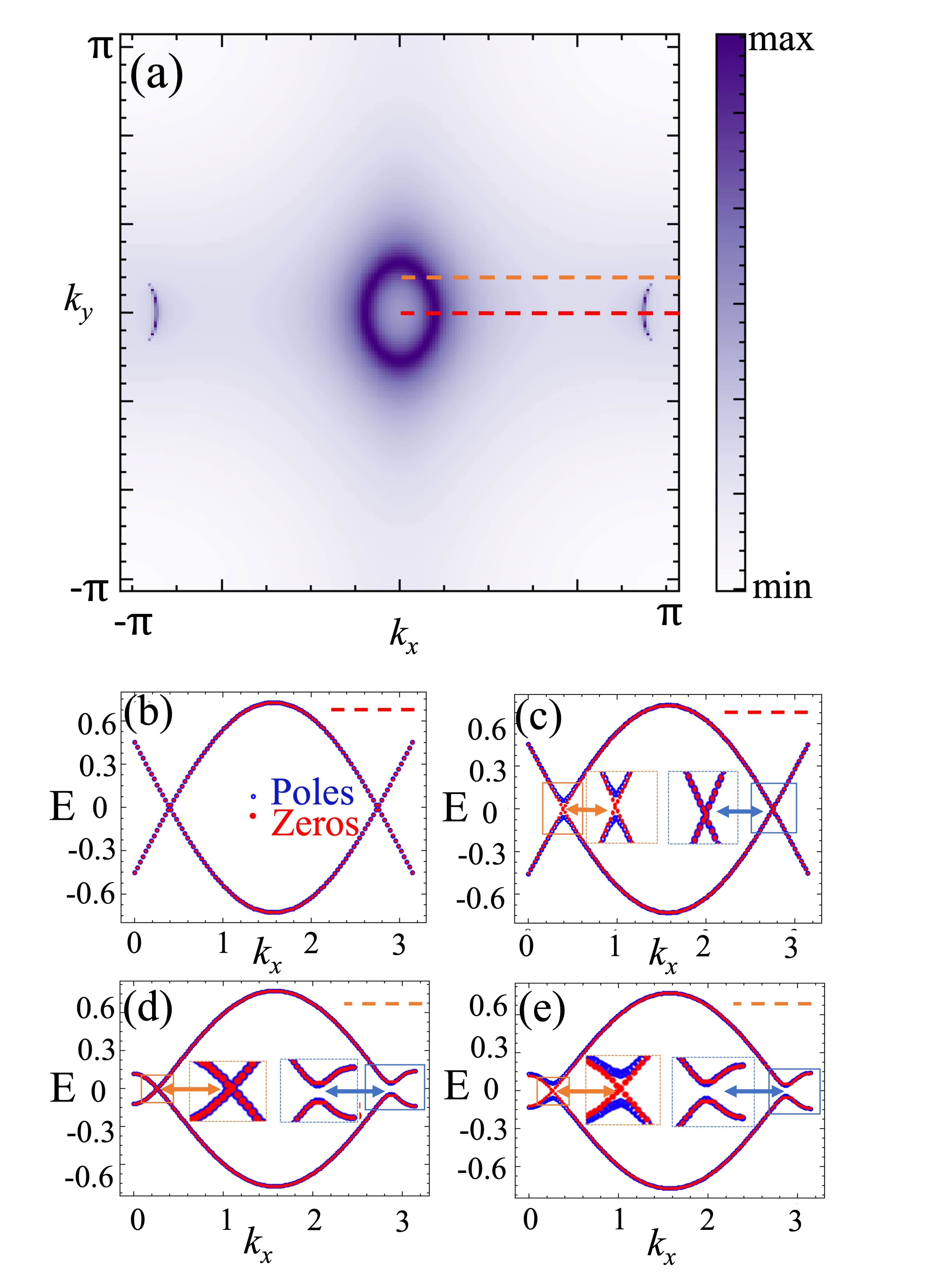
Similarly to the procedure for the TI, we recursively calculate surface Green’s function for the lattice model in the WSM phase. Fermi arcs emerge within the sBZ as illustrated in Fig.3(a), while Luttinger arcs defined by Green’s function zeros appear on top of the Fermi arcs, as shown in Fig.3 (b,d) for two values of . In the presence of s-wave surface superconductivity, either induced by proximity to another superconductor or intrinsically, as examined in recent works [20, 21, 22, 23], we can write the Bogoliubov-de Gennes (BdG) Hamiltonian as:
| (5) |
where the Hamiltonian is defined in the same manner as in Eq. (4), with parameters adjusted to represent the model in the WSM phase. Here, with acting on Nambu basis represents the superconducting pairing potential, which only has a non-zero value on the surface of the lattice model. As depicted in Fig.3 (c,e), the Fermi arcs near are gapped. However, the Luttinger arcs persist as anticipated.
Surface vs low-energy theory—Consider a gapped non-interacting topological phase on a slab. Conventionally, the gapped, plane waves are referred to as bulk states and the gapless, evanescent waves localized near the surface are called surface states. Besides being parametrically separated in energy, the two classes of eigenstates have vanishing overlap in the thermodynamic limit. Thus, naïvely, integrating out either high energy states and low energy states of the far surface, if any, or integrating out bulk degrees of freedom should produce identical descriptions of the near-surface physics in the thermodynamic limit. This logic also applies to gapless systems such as WSMs if one avoids projections of the bulk Weyl nodes in the sBZ.
We now prove this expectation incorrect. In particular, we show that the two approaches yield distinct values for thermodynamic properties, with the mismatch coming from LSs. Thus, the surface and bulk degrees of freedom are intimately coupled even though energy eigenstates traditionally associated with the surface and the bulk are separated in real space and in energy.
To see this mismatch explicitly, consider the single-particle free energy from a generic Green’s function , . Writing in terms of its poles and zeros , , gives the specific heat:
| (6) |
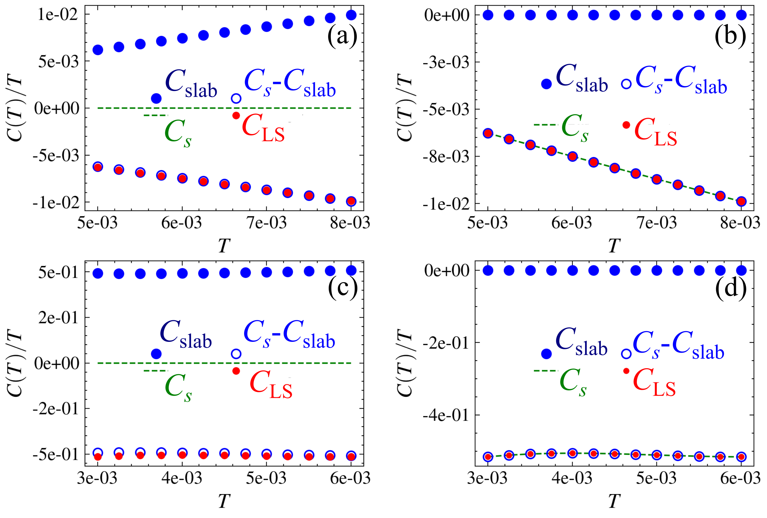
Clearly, only poles and zeros within contribute appreciably to . Evaluating at low using the full (), bulk () and effective surface () Green’s functions unveils the mismatch. In particular, for each point where the bulk plane waves and far-surface states are gapped with a gap and the near-surface is gapless, setting yields the specific heat from the near-surface states, as and are negligible. In contrast, choosing includes a negative contribution from the zeros or the LSs: , where . In fact, if the near-surface states are gapped out by a symmetry-breaking surface perturbation, then as while . Physically, the bizarre negative specific heat represents the reduction in total specific heat when the surface FSs of are gapped out upon coupling the new surface layer to via . Alternately, it can be viewed as the specific heat due to the appearance of the LS. We demonstrate these points numerically using lattice models for a TI and WSM in Fig. 4; for the latter, we separately calculate the specific heat of the gapless bulk states by applying periodic boundary conditions and subtract it from the total to isolate the Fermi arc contributions. As shown in Figs. 4(a,c), for the TI slab and WSM slab without the near-surface perturbation, while . After introducing surface perturbation, for both the TI and WSM slabs and , as shown in Figs. 4(b) and 4(d). In all cases, the difference, , matches the LS contribution. We assume the far surface is always gapped.
Application to —To effectively "detect" LSs in experiment, we propose examining the specific heat difference between a TI, [24], and the same TI with a thin film of [25, 26, 27, 28] deposited on top. Both and are van der Waals coupled layered materials; given the recent advancements in fabricating van der Waals heterostructures, depositing the latter on top of the former is conceivable. The thin film should ideally have an even number of layers; an odd-layer magnetic is a Chern insulator with edge states that also yield a contribution to the specific heat which must be subtracted off separately. In addition, the bare TI should be relatively thin so that the surface contribution to the specific heat is distinguishable from the bulk contribution – a nontrivial requirement since bare has bulk Fermi pockets. When is in its magnetized phase, the surface states of are expected to be gapped out, leading to a reduction in the specific heat. This reduction can alternately be interpreted as the negative specific heat due to the LSs that develop in the thin film upon coupling to the TI. In this setup, the thin film functions as the surface in the context of this work.
Summary — We demonstrated that in noninteracting topological phases of matter, LSs, formed by vanishing eigenvalues of the surface Green’s function, coexist with topological surface states. For instance, the surface of a TI hosts both a Dirac cone and a Luttinger cone, while a WSM surface accommodates Fermi and Luttinger arcs. Their coexistence is mandated by no-go theorems that the surface Green’s functions must obey but surface Hamiltonians evade in topological phases. Remarkably, surface perturbations that break the symmetries protecting the topological phase are unable to destroy the Luttinger surfaces even if they gap out the surface Fermi surfaces. We then show that surface LSs are absent in the low-energy theory of topological phases derived by integrating out higher-energy bulk states, but occur in the surface theory through the integration of bulk degrees of freedom. The existence of surface LSs is tightly connected to the bulk topology; thus, the absence of LSs in the low-energy theory of topological phases demonstrates that the surface theory is different from the low-energy theory, although they are naively considered equivalent. Our findings shed new light on the role of Green’s function zeros in topological condensed matter systems.
Acknowledgements.
The authors are grateful to Steven Kivelson and especially Hridis Pal for fruitful discussions. P.H. acknowledges support from National Science Foundation grant no. DMR 2047193 and K.C. acknowledges support from the Department of Energy grant no. DE-SC0022264.References
- Hasan and Kane [2010] M. Z. Hasan and C. L. Kane, Reviews of modern physics 82, 3045 (2010).
- Qi and Zhang [2011] X.-L. Qi and S.-C. Zhang, Reviews of Modern Physics 83, 1057 (2011).
- Volovik [2003] G. E. Volovik, The universe in a helium droplet, Vol. 117 (OUP Oxford, 2003).
- Armitage et al. [2018] N. P. Armitage, E. J. Mele, and A. Vishwanath, Rev. Mod. Phys. 90, 015001 (2018).
- Graf and Porta [2013] G. M. Graf and M. Porta, Communications in Mathematical Physics 324, 851 (2013).
- Rhim et al. [2018] J.-W. Rhim, J. H. Bardarson, and R.-J. Slager, Physical Review B 97, 115143 (2018).
- Volovik [2017] G. Volovik, Low Temperature Physics 43, 47 (2017).
- Mahan [2000] G. D. Mahan, Many-particle physics (Springer Science & Business Media, 2000).
- Fetter and Walecka [2012] A. L. Fetter and J. D. Walecka, Quantum theory of many-particle systems (Courier Corporation, 2012).
- Dzyaloshinskii [2003] I. Dzyaloshinskii, Physical Review B 68, 085113 (2003).
- Fabrizio [2022] M. Fabrizio, Nature communications 13, 1561 (2022).
- Wagner et al. [2023] N. Wagner, L. Crippa, A. Amaricci, P. Hansmann, M. Klett, E. König, T. Schäfer, D. Di Sante, J. Cano, A. Millis, et al., arXiv preprint arXiv:2301.05588 (2023).
- Zhao et al. [2023] J. Zhao, P. Mai, B. Bradlyn, and P. Phillips, Phys. Rev. Lett. 131, 106601 (2023).
- Bollmann et al. [2023] S. Bollmann, C. Setty, U. F. Seifert, and E. J. König, arXiv preprint arXiv:2312.14926 (2023).
- Blason and Fabrizio [2023] A. Blason and M. Fabrizio, Physical Review B 108, 125115 (2023).
- Obakpolor and Hosur [2022] O. E. Obakpolor and P. Hosur, Physical Review B 106, L081112 (2022).
- Giwa and Hosur [2021] R. Giwa and P. Hosur, Physical Review Letters 127, 187002 (2021).
- Sancho et al. [1985] M. L. Sancho, J. L. Sancho, J. L. Sancho, and J. Rubio, Journal of Physics F: Metal Physics 15, 851 (1985).
- Hosur and Qi [2013] P. Hosur and X. Qi, C. R. Phys. 14, 857 (2013), topological insulators / Isolants topologiques.
- Huang et al. [2019] C. Huang, B. T. Zhou, H. Zhang, B. Yang, R. Liu, H. Wang, Y. Wan, K. Huang, Z. Liao, E. Zhang, et al., Nature communications 10, 2217 (2019).
- Croitoru et al. [2020] M. D. Croitoru, A. Shanenko, Y. Chen, A. Vagov, and J. A. Aguiar, Physical Review B 102, 054513 (2020).
- Yi et al. [2024] H. Yi, Y.-F. Zhao, Y.-T. Chan, J. Cai, R. Mei, X. Wu, Z.-J. Yan, L.-J. Zhou, R. Zhang, Z. Wang, et al., Science 383, 634 (2024).
- Kuibarov et al. [2024] A. Kuibarov, O. Suvorov, R. Vocaturo, A. Fedorov, R. Lou, L. Merkwitz, V. Voroshnin, J. I. Facio, K. Koepernik, A. Yaresko, et al., Nature 626, 294 (2024).
- Zhang et al. [2009] H. Zhang, C.-X. Liu, X.-L. Qi, X. Dai, Z. Fang, and S.-C. Zhang, Nature physics 5, 438 (2009).
- Chen et al. [2009] Y. Chen, J. G. Analytis, J.-H. Chu, Z. Liu, S.-K. Mo, X.-L. Qi, H. Zhang, D. Lu, X. Dai, Z. Fang, et al., science 325, 178 (2009).
- Li et al. [2019] J. Li, Y. Li, S. Du, Z. Wang, B.-L. Gu, S.-C. Zhang, K. He, W. Duan, and Y. Xu, Science Advances 5, eaaw5685 (2019).
- Deng et al. [2020] Y. Deng, Y. Yu, M. Z. Shi, Z. Guo, Z. Xu, J. Wang, X. H. Chen, and Y. Zhang, Science 367, 895 (2020).
- He [2020] K. He, npj Quantum Materials 5, 90 (2020).
- Gurarie [2011] V. Gurarie, Physical Review B 83, 085426 (2011).
- Seki and Yunoki [2017] K. Seki and S. Yunoki, Physical Review B 96, 085124 (2017).
- Kotz and Timm [2023] M. Kotz and C. Timm, Phys. Rev. Res. 5, 033043 (2023).
- Zhou and Lee [2019] H. Zhou and J. Y. Lee, Physical Review B 99, 235112 (2019).
- Neupane et al. [2016] M. Neupane, N. Alidoust, M. M. Hosen, J.-X. Zhu, K. Dimitri, S.-Y. Xu, N. Dhakal, R. Sankar, I. Belopolski, D. S. Sanchez, et al., Nature communications 7, 13315 (2016).
Appendix for Robust Surface LSs in topological band structures
In Appendix A, we present two distinct methods for deriving an effective theory. Appendix B explains how the effective surface Green’s function can inherit the poles of the full Green’s function. In Appendix C, we show how the winding number confirms the presence of LSs on the surfaces of topological insulators. Appendix D explores the constraints imposed by time-reversal symmetry on the presence of poles and zeros in Green’s functions in fermionic systems, extending to generalized time-reversal symmetry in non-Hermitian systems. Appendix E provides a concise review of the recursive Green’s function technique used to calculate the surface Green’s function in the main text. Finally, Appendix F illustrates how to reconstruct the surface Green’s function from ARPES data.
Appendix A Surface theory vs low-energy
In this section, we contrast two approaches for deriving an effective theory – by explicitly integrating out the bulk degrees of freedom, which yields the surface Green’s function in Eq. 2 as a certain Schur complement, and integrating out high-energy states.
A.1 Integrating out bulk degrees of freedom
We begin with the Hamiltonian a -layer slab of a -dimensional topological phase with -dimensional surfaces:
| (7) |
We will use to denote Grassman variables for fermionic degrees of freedom on the "surface" and to denote the same for all the other fermions that we will concisely refer to as the "bulk". Integrals will be written in shorthand as . In this notation, the Euclidean path integrals for the bulk and full systems are and where
| (8) | ||||
| (9) | ||||
| (12) | ||||
| (15) |
Performing a standard Gaussian-Grassman integral over in yields an effective surface Green’s function :
| (16) | ||||
| (17) | ||||
| (18) |
The above expression is rather standard and has the form of a Dyson equation for the surface degrees of freedom with self-energy .
Alternately, we can obtain by straightforward linear algebra. Performing standard block matrix inversion of in the basis yields (suppressing frequency and momentum labels for brevity),
| (19) |
Clearly, is simply the sub-block of the corresponding to the surface degrees of freedom. In linear algebra parlance, is known as the Schur complement of in and simply denoted
| (20) |
In other words, integrating out yields the same effective surface Green’s functions as projecting the full Green’s function onto the -states.
A.2 Integrating out high-energy plane waves
In the parlance of topological condensed matter, "bulk" and "surface", respectively, refer to plane waves traversing the bulk at high energy and evanescent waves localized at a surface with exponential decay into the bulk layers. Strictly speaking, in a slab geometry, the energy eigenstates are standing waves traversing the slab and superpositions of evanescent waves localized on opposite surfaces. However, in the thermodynamic limit, traveling plane waves and evanescent waves on each surface become energy eigenstates. We will work in this limit for simplicity.
Now, an alternate derivation of the effective surface theory by integrating out the plane waves is justified. Explicitly, we can spectrally decompose the total Hamiltonian as
| (21) |
where , and denote energies of the evanescent waves on the surface under consideration, evanescent waves on the opposite surface of the slab, and plane wave states, respectively. As the various sets of states are decoupled, integrating out the plane waves and far-surface evanescent waves is trivial and we are left with effective Hamiltonian and Green’s function for the near surface:
| (22) | ||||
| (23) | ||||
| (24) |
in the basis of , where is the number of degrees of freedom defined as the surface.
Appendix B Inheritance of surface poles by the surface Green’s function
In this section, we prove that the effective surface Green’s function studied in this paper inherits surface poles from the full Green’s function , i.e., poles from the latter whose corresponding eigenfunctions have finite support on the surface degrees of freedom.
Similarly to , we can spectrally decompose as
| (25) |
Now, the plane waves and far-surface evanesccent waves have a vanishing amplitude on the near surface in the thermodynamic limit. Thus, projecting onto the near surface gives
| (26) |
where are basis states spanning the near surface. Taking the trace gives
| (27) |
Clearly, every surface pole of , where vanishes with being finite, causes to diverge, indicating a pole in an eigenvalue of .
Appendix C Identifying the LSs through the topological winding number
The stability of the FS is derived from the topological property of the single-particle Green’s function with and denoting the Bloch momentum and imaginary frequency [3]. The corresponding topological invariant is a winding number defined as follows:
| (28) |
where denotes a counterclockwise loop in the -space, and tr is the trace over spin, orbital, or other indices. The winding number can also be expressed as . Considering a simple single-particle Green’s function with Fermi velocity and Fermi momentum , the resulting winding number is expressed as , where is the linking number between the loop and the FS.
On the other hand, when the single-particle Green’s function’s zeros are zero, they define the LS, where the Green’s function can be approximated as with Luttinger momentum . The resulting winding number is expressed as , where represents the link number between the loop and the LS.
In this section, we demonstrate the utility of the winding number in identifying the presence of zeros in the surface Green’s function. For the model considered in the previous section, numerical calculations reveal that the unperturbed surface Green’s function exhibits overlapped zeros and poles, as illustrated in Fig. 2(a). Consequently, the winding number is zero due to the cancellation between zeros and poles. Upon introducing a surface perturbation to eliminate the poles, the winding number for a loop with an imbalanced count of oppositely moving zeros attains a nonzero integer value. This value equals the difference between the numbers of left-moving and right-moving zeros within the loop.
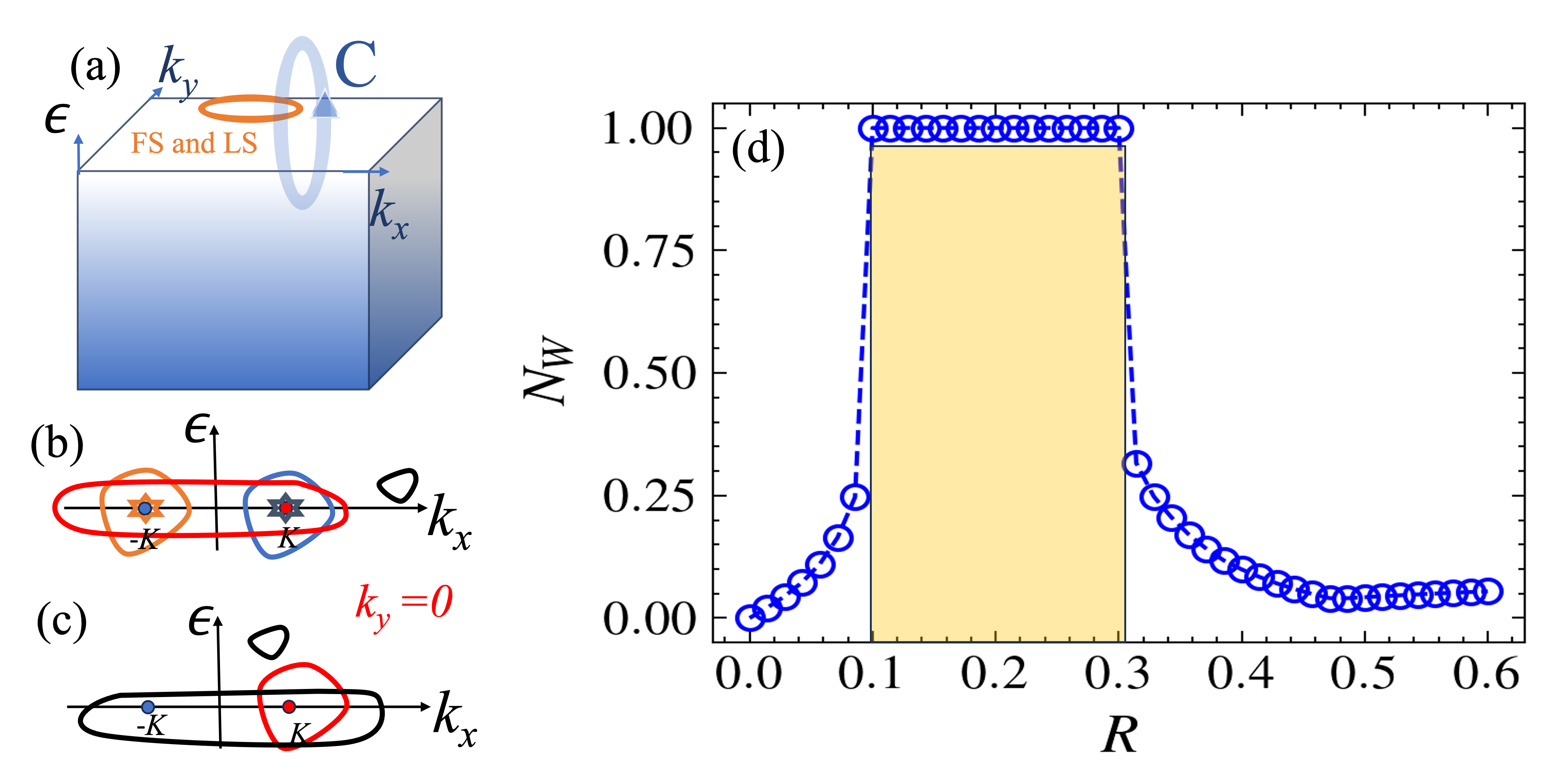
To validate this assertion, we examine the surface Green’s function obtained from the lattice model in the topological insulating phase with a nonzero chemical potential. In this scenario, the Dirac points and Luttinger points evolve into Dirac circles and Luttinger circles, respectively. Without loss of generality, we choose loops in the -plane. For the unperturbed surface, there exists a right-moving () pole and a right-moving zero at the point , as well as a left-moving () pole and a left-moving zero at the point —illustrated schematically in Fig. S1 (b). Consequently, the winding number is zero for any loop in the -plane in this case.
For the perturbed surface, the poles are gapped out, but the right-moving and left-moving zeros persist at the same points (Fig. S1 (c)). We focus on a loop characterized by points with . The winding number is illustrated in Fig. S1 (d), showing for the radius (within the yellow rectangle). This range includes only a single right-moving zero inside the loop. The winding number becomes zero for since no zeros are included inside the loop, and for because both a left-moving and a right-moving zero are included inside the loop. In our numerical calculation, we use the parameter values and .
Appendix D Restrictions on zeros and poles by Time reversal symmetry
For a single-particle Green’s function, its determinant satisfies the following general equation [29, 30]:
| (29) |
where represents a complex number, while and be the zero and pole of a single-particle Green’s function at Bloch momentum , respectively. It’s important to note that and are real-valued quantities. We then define the set and , where is unit direction vector along the directed loop, we adopt a counterclockwise direction as the loop orientation throughout this work, without loss of generality. We categorize the points in set as left-moving zeros, and those in set as right-moving zeros. Similarly, points in set are labeled as left-moving poles, and those in set as right-moving poles. The number of elements in a set is denoted by .
On the other hand, symmetries can relate the Green’s function at different positions in the BZ, leading to band degeneracy. Consequently, symmetries can impose constraints on the properties of the Green’s function. In this section, we consider time-reversal symmetry (), where denotes complex conjugate, as a specific example to illustrate its influence on the properties of the Green’s function.
The time-reversal symmetry dictates that the Green’s function satisfies the equation [31]:
| (30) |
where represents the unitary part of the time-reversal operator and denotes transposition. This symmetry denoted as type C symmetry of Class 7 in Ref. [32], which guarantees that for each eigenstate of , there is an associated pair with the same complex eigenvalue, providing robust Kramers degeneracy at time-reversal invariant momenta. Incorporating this symmetric Green’s function, we propose the following proposition:
Proposition: If the loop in the BZ is a time-reversal-invariant closed line, e.g., and in the BZ, then .
Proof.
The antisymmetric unitary matrix of the antiunitary time reversal symmetry operator implies that the dimension of the Green’s function is even. Additionally, for the type C symmetry of Class 7, the generalized Kramers degeneracy ensures that all eigenvalues of the Green’s function come in pairs with opposite chiralities[32]. Therefore, one has:
| (31) |
where and are the dimension and eigenvalues of the Green’s function , respectively. ∎
It’s worth noting that in the above proof, we don’t assume the system to be noninteracting. Therefore, the restriction on the number of zeros and poles of the Green’s function holds true for interacting many-body Fermionic systems with time-reversal symmetry as well.
Appendix E Recursive methods for the surface Green’s function
In this section, we provide a brief overview of the recursive Green’s function used to obtain the surface Green’s function in the main text. More details can be found in the reference ([18]).
For a solid with a surface, it can be described by a semi-infinite stack of layers with nearest-neighbor inter-layer interaction. Without loss of generality, let’s set the boundary at z=0, and the bulk extends in the positive z direction. The lattice periodicity on the (x, y)-plane is preserved. Thus, is a good quantum number, and each layer can be described by the Bloch wavefunctions with n denoting the layer indices. Taking matrix elements of between the Bloch wavefunctions, one has the equations for each :
| (32) |
where the matrices
| (33) |
and is the unit matrix. Since each layer is described by the same Hamiltonian and the same coupling between nearest neighbor layers, one has and . From Eq. (32), we get
| (34) |
where
| (35) |
Equations (34) define a chain that couples the Green’s function matrix elements with even indices only. Equations (35) define an effective Hamiltonian describing a chain with a lattice constant twice the original lattice, and the effective intra-layer and inter-layer hopping are renormalized. Starting from Eq. (34) and repeating the same procedure n times, we get
| (36) |
where is obtained by performing the following iteration n times, ensuring that and can be made as small as desired,
| (37) |
where , and . After n iterations, the surface layer is equivalent to the original surface layer coupled to layers.
Appendix F Reconstruction of surface Green’s function
In this section, we use a lattice model in the topological insulating phase as an example to illustrate the reconstruction of the surface Green’s function with components , where and label the spin indices. We emphasize that although this method can, in principle, reconstruct the surface Green’s function, it is challenging to implement with current techniques. For example, spin-resolved ARPES data [33] provides diagonal components of the imaginary part of the surface Green’s function; however, to our knowledge, the off-diagonal components have not yet been observed experimentally.
Firstly, we employ the recursive method to obtain the surface Green’s function and extract its imaginary part, which constitutes the spectral function that can be approximated by ARPES data. Secondly, the Kramers-Kronig relations: , are utilized to obtain the real part of the surface Green’s function and where denotes the Cauchy principal value. Generally, a larger number of spectral function values across frequencies is required to accurately determine the real part of the surface Green’s function, but in principle, this is feasible. Finally, by combining the real part of the surface Green’s function with the ARPES data, we reconstruct the complete surface Green’s function .
In Table I, we present the minimum value of the singular values of the reconstructed surface Green’s function for the TI, where the surface Dirac cone is gapped by a surface perturbation breaking time-reversal symmetry. The integration in the Kramers-Kronig relations is performed from -3 to 3, which is larger than the bandwidth of the lattice model, and the integration step is . The deviation of singular values of the reconstructed surface Green’s function from the singular values of the actual surface Green’s function indicates that a larger number of data points of the spectral function are needed to obtain a faithfully reconstructed surface Green’s function.
| 5 | 5 | |||
|---|---|---|---|---|
| 4.98 | 4.98 | 0.018 | 0.018 |