Robust subgroup-classifier learning and testing in change-plane regressions
Abstract
Considered here are robust subgroup-classifier learning and testing in change-plane regressions with heavy-tailed errors, which can identify subgroups as a basis for making optimal recommendations for individualized treatment. A new subgroup classifier is proposed by smoothing the indicator function, which is learned by minimizing the smoothed Huber loss. Nonasymptotic properties and the Bahadur representation of estimators are established, in which the proposed estimators of the grouping difference parameter and baseline parameter achieve sub-Gaussian tails. The hypothesis test considered here belongs to the class of test problems for which some parameters are not identifiable under the null hypothesis. The classic supremum of the squared score test statistic may lose power in practice when the dimension of the grouping parameter is large, so to overcome this drawback and make full use of the data’s heavy-tailed error distribution, a robust weighted average of the squared score test statistic is proposed, which achieves a closed form when an appropriate weight is chosen. Asymptotic distributions of the proposed robust test statistic are derived under the null and alternative hypotheses. The proposed robust subgroup classifier and test statistic perform well on finite samples, and their performances are shown further by applying them to a medical dataset. The proposed procedure leads to the immediate application of recommending optimal individualized treatments.
Keywords: Gaussian-type deviation; Heavy-tailed data; Nonstandard test; Robust classifier; Subgroup classifier; Subgroup detection.
1 Introduction
When studying the risk of a disease outcome, there could be heterogeneity across subgroups characterized by covariates, meaning that the same treatment in different subpopulations may cause different treatment effects of predictors. In the presence of population heterogeneity in classical models, learning the subgroup classifier and testing the existence of subgroups associated with the risk-model heterogeneity are important for understanding better the different effects of predictors and modeling better the association of diseases with predictors. In precision medicine, this plays a core role in guiding personalized treatment to individuals in a population by identifying subgroups with different treatment effects on disease. There has been much previous research on learning the subgroup classifiers of individuals based on various models Foster et al., (2011); Wei and Kosorok, (2018); Huang et al., (2020); Li et al., (2021); Zhang et al., (2022).
Before learning the subgroup classifier, it is necessary to test for the existence of subgroups of individuals to address the potential risk of finding false-positive subgroups. This necessity not only arises from the data themselves but is also intrinsic to statistics, because the nonexistence of subgroups causes the identifiability problem when learning the subgroup classifier. However, this test problem belongs to the class of nonstandard tests with loss of identifiability under the null hypothesis; see Wald, (1943); Andrews and Ploberger, (1994, 1995); Davies, (1977); Song et al., (2009); Liu et al., (2024); Kang et al., (2024), among others. Therefore, the focus herein is on learning the subgroup classifier and testing for the existence of subgroups simultaneously, which offers more information and the potential for making the best recommendations for optimal individualized treatments and guiding future treatment modification and development.
Let be the observed data, which are independent and identically distributed copies of . Consider the regression model with change plane Lee et al., (2011); Zhang et al., (2022); Mukherjee et al., (2022); Liu et al., (2024)
| (1) |
where , and are unknown parameters, and and for some . When , the error has a finite second moment, denoted by . For easy expression, let . Following the expressions in Liu et al., (2024), is called the grouping variable, is called the grouping parameter, is called the grouping difference variable, is called the grouping difference parameter, is called the baseline variable, and is called the baseline parameter. Herein, the indicator function is called the subgroup classifier.
The technology for collecting and processing data sets has improved considerably in recent years, and one is now more likely to encounter heavy-tailed or low-quality data, thereby causing the typical assumption of a Gaussian or sub-Gaussian distribution to fail. Therefore, new challenges arise compared with the classic methodology for modeling non-Gaussian or heavy-tailed data. Even for linear regression models with heavy-tailed errors, the ordinary least squares (OLS) estimators are suboptimal both theoretically and empirically. Instead, proposed herein is a robust estimator of subgroup classification by considering the change-plane model (1) with heavy-tailed errors. This paper addresses two important problems for model (1) with heavy-tailed errors, i.e., subgroup-classifier learning (Section 2) and subgroup testing for whether subgroups exist (Section 3).
1.1 Robust subgroup-classifier learning
Li et al., (2021) considered the change-plane model (1) with Gaussian errors. Also, Zhang et al., (2022) investigated a quantile regression with a change plane and derived the asymptotic normalities for the grouping difference parameter and the grouping parameter. However, although quantile or median regression models require no Gaussian or sub-Gaussian assumption, they essentially estimate the conditional quantile or median regression instead of the conditional mean regression. If the mean regression is of interest in practice, then these procedures are not feasible unless the error distribution is symmetric around zero, which may be too strong to cause the misspecification problem. See Fan et al., 2017b for some examples that demonstrate the distinction between conditional mean regression and conditional quantile or median regression.
Linear regression models with heavy-tailed errors are prevalent in the literature. Fan et al., 2017b proposed a robust estimator of high-dimensional mean regression in the absence of asymmetry and with light tail assumptions. Zhou et al., (2018) provided a robust M-estimation procedure with applications to dependence-adjusted multiple testing. Sun et al., (2020) and Wang et al., (2021) studied adaptive Huber regression for linear regression models with heavy-tailed errors. Chen and Zhou, (2020) investigated robust inference via multiplier bootstrap in multiple response regression models, constructing robust bootstrap confidence sets and addressing large-scale simultaneous hypothesis testing problems.


Mukherjee et al., (2022) studied the change-plane problem under heavy-tailed errors when and , which is a special case of the change-plane model (1), and they left the general change-plane model with heavy-tailed errors for future work. Herein, a new robust procedure is introduced to estimate parameters and consequently to learn the subgroup classifier. Figure 1 shows boxplots of the estimation errors of the parameter with norm and the accuracies of the estimated subgroup classifier, where the norm of the estimation errors is defined as with the robust estimator of the true grouping parameter , and the accuracy is defined as with the robust estimator of the true parameter . Here, the settings are and with 1000 repetitions, the heavy-tailed errors are generated from the Pareto distribution with shape parameter 2 and scale parameter 1, and and and are generated independently from multivariate normal distributions and , respectively; see Section 4 for details. As used by Zhang et al., (2022), the smooth function with smoothness parameter is chosen, and the proposed robust estimation procedure (AHu) is compared with the method based on OLS (Li et al., 2021). Figure 1 sends the important message that in the presence of heavy tails, compared with the existing method (Li et al., 2021), the proposed robust estimators not only reduce the estimation error dramatically but also improve significantly the accuracy of the subgroup classifier.
1.2 Robust subgroup testing
Another goal of this paper is to test for the existence of subgroups, i.e.,
| (2) |
Note that the grouping parameter is not identifiable under the null hypothesis.
The classic Wald-type test or score-based test is powerful in standard test problems when there is no identifiability problem in both the null and alternative hypotheses, but these common procedures are not feasible when nuisance parameters are present. Andrews and Ploberger, (1994) and Andrews and Ploberger, (1995) studied the weighted average exponential form, which was originally introduced by Wald, (1943). Davies, (1977) investigated well the supremum of the squared score test (SST) statistic for mixture models, which was applied by Song et al., (2009) and Kang et al., (2017) to semiparametric models in censoring data.
All the aforementioned testing methods are optimal tests based on the weighted average power criterion. However, because these optimal tests take the weighted exponential average of the classical tests over the grouping parametric space , they may not only not perform well in practice when the dimension of is large but also give rise to a heavy-burden calculation of the p-value or the critical value. Instead, Liu et al., (2024) introduced a new test statistic by taking the weighted average of the SST (WAST) over and removing both the inverse of the covariance and the cross-interaction terms to overcome the drawbacks of SST. Thanks to its closed form, WAST achieves more-accurate type-I errors and significantly improved power and hence dramatically reduced computational time as a byproduct.


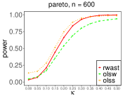
All the aforementioned test procedures require the important assumption of Gaussian or sub-Gaussian errors in the change-plane models, none of which apply to heavy-tailed data sets. Therefore, proposed herein is a robust test procedure based on WAST (Liu et al., 2024), called robust WAST (RWAST). Figure 2 shows the power curves of the proposed RWAST, WAST as introduced by Liu et al., (2024), and SST as considered by Davies, (1977); Kang et al., (2017). A total of 1000 bootstrap samples is set, and the other settings are the same as those in Section 1.1. With the nominal significance level , the type-I errors for these three methods are for , for , and for . It follows that RWAST controls the type-I errors well, while those of SST based on quadratic loss are larger and deviate far from 0.05. Figure 2 shows that in the presence of heavy tails, the proposed RWAST achieves larger power in comparison with WAST based on the ordinary quadratic loss.
In summary, from the demonstration examples in Section 1.1 and Section 1.2, compared with the existing nonrobust methods for heavy-tailed data, the proposed robust estimation procedure is characterized by lower estimation errors and higher accuracy, and the robust test procedure has more-accurate type-I errors and larger power.
1.3 Main contributions
The main contributions of this paper are summarized as follows. First, the robust estimation procedure for the change-plane model (1) with heavy-tailed errors is investigated carefully. The proposed robust estimator adapts to the sample size, the robustification parameter in the Huber loss, the smoothness parameter when approximating the indicator function in the subgroup classifier, and the moments of errors. The sacrifices made in pursuit of robustness and smoothness are analyzed theoretically, with the bias involving the robustification parameter arising from the pursuit of robustness, and the one involving the smoothness parameter arising from the approximation to the indicator function. The nonasymptotic properties for parameters and are established, as well as those for the grouping parameter. The theoretical results reveal that the proposed estimators of the grouping difference parameter and baseline parameter have Gaussian-type deviations (Devroye et al., 2016). Also provided is the nonasymptotic Bahadur representation of the proposed robust estimators, which is convenient for deriving the classical asymptotic results needed for statistical inference such as hypothesis tests and constructing confidence regions. Extensive simulation studies show that the proposed robust estimation procedure is superior to its several competitors.
Second, for the change-plane model with heavy-tailed errors, RWAST is proposed, which makes full use of the data’s heavy-tailed information and overcomes the drawbacks of loss of power in practice and the heavy computational burden of SST when the dimension of the grouping parameter is large. The asymptotic distributions of the proposed RWAST under the null and alternative hypotheses are established based on the theory of degenerate U-statistics. As with exponential average tests, the proposed asymptotic distributions are not standard (e.g., the normal or distribution), so a novel bootstrap method that is easily implemented and theoretically guaranteed is introduced to mimic the critical value or p-value. Comprehensive simulation studies conducted with finite sample sizes and for various heavy-tailed error distributions show the excellent performance of the proposed RWAST, which improves the power significantly and reduces the computational burden dramatically.
In summary, a novel robust estimator is proposed that adapts to the sample size, dimension, robustification parameter, moments, and smoothness parameter in pursuit of the optimal tradeoff among bias, robustness, and smoothness. To the best of the author’s knowledge about change-plane analysis, the literature contains no nonasymptotic results with sub-Gaussian tails for parameters and , and no nonasymptotic results with sub-exponential tails for the Bahadur representation of these parameters. Furthermore, a robust test procedure is proposed that improves on WAST in the change-plane model with heavy-tailed errors.
1.4 Notation and Organization of paper
Here, some useful notation is introduced for convenience of expression. For a vector and a square matrix , denote by the Euclidean norm of , by the trace of ; and . Denote by the induced operator norm for a matrix .
Denote by the ordinary probability measure such that for any measurable function , by the empirical measure of a sample of random elements from such that , and by the empirical process indexed by a class of measurable functions such that for any . Let be the space of all measurable functions such that , where and denotes the essential supremum when . Let be an -covering number of with respect to the seminorm , where is a class of measure functions and is finite discrete.
The remainder of this paper is organized as follows. Section 2 provides the robust estimators for the grouping difference parameter and grouping parameter as well as the subgroup classifier, and theorems reveal that these estimators achieve Gaussian-type deviations. Also derived is the Bahadur representation of the robust estimators, and it is shown that the remainder of the Bahadur representation achieves sub-Gaussian tails. Section 3 presents the RWAST statistic and establishes its limiting distributions under the null and alternative hypotheses. Section 4 reports the results of simulation studies conducted to evaluate the finite-sample performance of the proposed methods with competitors in the change-plane models with heavy-tailed errors. The performance of the proposed methods is illustrated further by applying them to a medical dataset in Section 5. Finally, Section 6 concludes with remarks and further extensions. The proofs are provided in the Supplementary Material, and an R package named “wasthub” is available at https://github.com/xliusufe/wasthub.
2 Robust subgroup-classifier learning
In this section, the subgroup classifier is learned to partition subjects into two subgroups, and nonasymptotic properties are provided for the robust estimators, whose deviations achieve sub-Gaussian tails. To adapt for different magnitudes of errors and to robustify the estimation, the Huber loss (Huber, 1964; Fan et al., 2017b ; Wang et al., 2021; Han et al., 2022) is considered, the definition of which begins this section.
Definition 2.1.
The Huber loss is a hybrid of the squared loss with small errors and absolute loss for large errors. Denoting by the ordinary quadratic loss, it is straightforward to see that .
2.1 Robust estimation
Rewrite model (1) as
| (6) |
where , with . To avoid the identifiability problem for , is assumed in this section. Denote , where is the product space.
Because the indicator function is not differentiable, it is natural to approximate it by a smooth function satisfying
Note that this smooth function characterizes the cumulative distribution function instead of the density function; see Seo and Linton, (2007); Li et al., (2021); Zhang et al., (2022); Mukherjee et al., (2020) for more details. The literature contains many commonly used smooth functions, such as the cumulative distribution function of standard normal distribution , the sigmoid function , and the mixture of the cumulative distribution function and density of standard normal distribution . Thus, model (6) can be approximated by
| (7) |
where , and is a predetermined tuning parameter associated with satisfying , called the smoothness parameter.
For any , let be the minimizer defined as
| (8) |
which approximates the minimizer
| (9) |
As did Sun et al., (2020), is called the Huber coefficient, which usually distinguishes from the true parameter . Measured by , the Huber error is caused by the robustification for the heavy-tailed errors, while the distance is a consequence of both robustification and smoothness. Theorem 2 reveals that is controlled by both and , with playing the role of the bandwidth in the nonparametric area.
Minimizing the empirical loss in (8) produces the robust estimator of interest, i.e.,
| (10) |
From (8), (9), and (10), the total estimation error can be decomposed into three parts, i.e.,
| (11) |
It is natural to use the alternating strategy to obtain the estimate, denoted by . Specifically, the parameters and can be estimated iteratively as follows. For given , and are obtained by minimizing
and for given and , is estimated by minimizing
Iterating these two maximizers leads to the desired robust estimator. The above alternating strategy is summarized in Algorithm A in Appendix A of the Supplementary Material.
2.2 Nonasymptotic properties
This section begins with assumptions needed to establish the nonasymptotic properties. Let be by removing , i.e., , and and .
-
(A1)
The conditional random vectors and given are sub-Gaussian, and is sub-Gaussian. There is a universal constant satisfying , , and . For any , the matrices , , and are uniformly positive definite, and there is a universal constant satisfying , , and .
-
(A2)
The error variable is independent of and satisfies and with . Denote .
-
(A3)
for any , and there is a constant satisfying .
-
(A4)
For almost every , the density of conditional on is everywhere positive. The conditional density of given has continuous derivative, and there is a constant such that and are uniformly bounded from above by over . is uniformly bounded from below by over , and is uniformly bounded from above by over , where and are constants.
-
(A5)
The smooth function is twice differentiable and . is symmetric around zero. Moveover, there is a universal constant satisfying with .
Remark 1.
Assumptions (A1)–(A5) are mild conditions for deriving the nonasymptotic bounds in Theorems 1–4 below. Assumption (A1) is the moment condition for covariates. Assumption (A2) is imposed to control the moment of error and to yield the adaptive nonasymptotic upper bounds; see Fan et al., 2017b ; Wang et al., (2021); Han et al., (2022). Assumption (A3) is mild and easily verified in practice, and it is usually imposed in change-plane analysis; see Kang et al., (2017); Liu et al., (2024). Assumption (A4) is required to establish nonasymptotic properties in dealing with the indicator function; see Horowitz, (1993); Zhang et al., (2022). By Lemmas C1–C3 in Appendix C of the Supplementary Material, Assumption (A5) holds for commonly used smoothing functions such as (i) the cumulative distribution function of standard normal distribution , (ii) the sigmoid function , and (iii) the function ; see Horowitz, (1993); Zhang et al., (2022).
Theorem 1.
Let . If Assumptions (A1)–(A4) hold, then for some , the minimizer given in (9) satisfies
and
where is a constant.
Theorem 1 states that the Huber error is of order for and of order for . As tends to infinity, because the Huber loss becomes the ordinary quadratic loss, the Huber error vanishes as expected. The next theorem studies the smooth error and Huber loss together.
Theorem 2.
If Assumptions (A1)–(A5) hold, then for some and , the minimizer given in (8) satisfies
and
where is a constant.
Theorem 2 reveals that and are associated with both the Huber error and the smooth error. The smoothness parameter can be of order , and because approximates as tends to zero, the upper bounds in Theorem 2 are of the same order as those in Theorem 1 when . Thus, the deviations and are sacrifices in pursuit of robustification and smoothness. The next theorem provides the exponential-type deviations for the baseline and grouping difference parameters and grouping parameter.
Theorem 3.
If Assumptions (A1)–(A5) hold, then for some and any , when and , the estimator given in (10) satisfies, with probability at least ,
| (12) | ||||
and
| (13) | ||||
where is a constant depending on only the constants , and
With appropriate choice of with , such as with , the nonasymptotic property of the sub-Gaussian estimator in Theorem 3 demonstrates that the deviation adapts to the sample size, dimension, robustification parameter , and moments in pursuit of the optimal tradeoff between bias and robustness, and the deviation adapts to the extra smooth parameter to achieve smoothness. Adaptation to the robustification parameter is caused by pursuing the robustness for linear regression with heavy-tailed errors. The deviations and coincide with the smoothed OLS estimator when , because as . The next theorem derives the nonasymptotic Bahadur representation of the robust estimators given in (10).
Theorem 4.
Theorem 4 shows that the remainder of the Bahadur representation of achieves the rate , which is the same as that for . Because of the rate restriction and , the remainder of the Bahadur representation in inequality (15) does not exhibit subexponential behavior as considered by Sun et al., (2020); Chen and Zhou, (2020). This reason is that there is a change plane involved a smooth function in model (1). To the best of the authors’ knowledge, this is the first time that this type of nonasymptotic Bahadur representation has been reported in the literature, especially for the robust estimator of the grouping parameter, with previous studies reporting only polynomial-type deviation bounds; see Liu et al., (2024); Zhang et al., (2022). It is convenient to derive the classical asymptotic results from the Bahadur representation, and Theorems 3 and 4 show that the robustification parameter and the smoothness parameter play the same role as bandwidth in constructing classical nonparametric estimators.
2.3 Implementation
The theoretical properties in Section 2.2 guarantee that the robust estimation performs well with appropriate choices of the robustification parameter and the smoothness parameter . Because the robustification parameter is treated as a tuning parameter to balance bias and robustness, it is natural to consider using the cross-validation (CV) method to select an appropriate in practice. However, as noted by Chen and Zhou, (2020) and Wang et al., (2021), because is typically unknown in practice, its empirical OLS estimator is poor when the errors are heavy-tailed. Instead, there are two good alternatives (Chen and Zhou, 2020): (i) an adaptive technique based on Lepski’s method Lepskii, (1992) and (ii) a Huber-type method by solving a so-called censored equation Hahn et al., (1990); see Chen and Zhou, (2020); Wang et al., (2021) for details. For the smoothness parameter , the CV method is always a natural choice for selecting an appropriate one. Alternatively, from the theoretical conditions on the smoothness parameter , a rule of thumb suggested by Seo and Linton, (2007), Li et al., (2021), and Zhang et al., (2022) is recommended by considering the computation reduction, where is a constant and is the estimated standard deviation of , with being the estimator of by using ordinary quadratic loss.
Attention now turns to the implementation for subgroup-classifier learning, with the parameters and estimated iteratively as follows. Let be the loss function for model (1), i.e.,
and let the smoothed loss function be
| (16) |
For given , one obtains and by minimizing the smoothed loss function
and for given and , one estimates by
Iterating these two minimizers leads to the desired robust estimators. These are summarized with the multiplier bootstrap calibration in Algorithm 1 in Appendix A of the Supplementary Material, which provides the strategy for estimating the confidence intervals for the estimators , , and .
Note that herein, and for given are obtained by a robust data-adaptive method proposed by Wang et al., (2021). Specifically, is estimated and is calibrated simultaneously by solving the following system of equations:
where , , and as suggested by Wang et al., (2021). The initial values and are set using the ordinary quadratic loss, where , with being the estimator of .
3 Robust subgroup testing
Before learning the subgroup classifier, it is of interest to test for the existence of subgroups, which guarantees avoidance of the identifiability problem of . This section considers the test problem (2). Recall the loss function in (9), i.e.,
| (17) |
the derivative of which with respect to under the alternative hypothesis is
and with respect to under the null hypothesis is
where is the first derivative of the Huber loss (5), defined as .
3.1 Robust estimation under null hypothesis
Under the null hypothesis, model (1) reduces to the ordinary linear regression model with heavy-tailed errors, i.e.,
| (18) |
Parametric estimation in model (18) is well-studied in the literature; see Huber, (1964, 1973); Fan et al., 2017b ; Sun et al., (2020); Wang et al., (2021); Han et al., (2022); Chen and Zhou, (2020); Zhou et al., (2018), among others. Let be the estimate of under the null hypothesis, i.e.,
| (19) |
Before establishing asymptotic properties for the robust estimator under the null hypothesis and the test statistic, the following required assumptions are made.
-
(B1)
The random vector is sub-Gaussian, is a finite and positive definite deterministic matrix, and there is a universal constant satisfying , .
-
(B2)
The error variable is independent of and satisfies and with .
-
(B3)
for any .
Remark 2.
Assumption (B1) is the moment condition of covariates for establishing the nonasymptotic properties under the null hypothesis and deriving the asymptotic distributions. Assumption (B2) is the same as Assumption (A2), and Assumption (B3) is the same as Assumption (A3).
3.2 Robust test statistic
As discussed by Liu et al., (2024), for any known , it is natural to consider an SST statistic for testing , i.e.,
| (21) |
where is given in (19) and . Here, and are consistent estimators of and , respectively, where is as defined in Assumption (B1) and
Lemma 2.
If Assumptions (B1)–(B3) hold, then for any fixed , converges in distribution to a one with degrees of freedom under as .
Although there is an unknown parameter that prevents from being used directly in practice, Lemma 2 reveals essentially that the asymptotic distribution of is free of the nuisance parameter . Thus, the supremum and the weighted average of over should guarantee the correct type-I errors, which motivates constructing the robust test statistic based on the weighted average of over the parametric space .
Fan et al., 2017a studied the supremum of the SST statistic (SST) over the grouping parameter for a semiparametric model, i.e.,
| (22) |
The test statistic has been investigated widely in the literature; see Andrews and Ploberger, (1994, 1995); Davies, (1977); Song et al., (2009); Shen and Qu, (2020); Liu et al., (2024). It is easy to extent the SST to model (1) with heavy-tailed errors according to the Bahadur representation in Theorem 4.
When the dimension of the parametric space is large, searching for the supremum value over may cause to lose power in practice and is time-consuming computationally. To avoid these drawbacks, proposed in this section is a robust test procedure that is a type of WAST statistic first introduced by Liu et al., (2024).
Proposed herein is RWAST, i.e.,
| (23) |
where
| (24) |
and . As noted by Liu et al., (2024), there is a Bayesian explanation for the weight . In fact, Lemma D1 in the Supplementary Material shows that
where is the standard multi-Gaussian density and can be chosen as another weight satisfying for all and . In the Bayesian motivation, the grouping parameter has a prior with density . Because the goal herein is to test for the existence of subgroups instead of estimating the grouping parameter, the difference is that there is no requirement for the posterior distribution.
The choice of the weight affect the computation of the test statistic because of the numerical integration over . Thus, taking the weight as the standard multi-Gaussian density offers good performance in practice, as illustrated in the simulation studies in Section 4 and the case studies in Section 5. To illustrate the performance in robust regression, numerical studies were conducted to investigate the sensitivity of the weight’s choice by comparing with the closed form in (24) and the approximated in (E.3) of Appendix E.3 in the Supplementary Material. From the numerical results, compared with the approximated , the test statistic with in (24) has higher power uniformly and takes only 10% of the time computationally when . This is a strong recommendation to use the closed-form RWAST in (24).
To establish the asymptotic distribution of RWAST, additional notation is introduced below. Denote the kernel of a U-statistic under the null hypothesis by
| (25) | ||||
where , and
with .
Theorem 5.
If Assumptions (B1)–(B3) hold, then under the null hypothesis, we have
where denotes convergence in distribution, , is a random variable of the form , and are independent variables, i.e., has the characteristic function
Here, is the imaginary unit, and are the eigenvalues of the kernel under , i.e., they are the solutions of for nonzero , where is the density of .
Investigated next is the power performance of the proposed test statistic under two types of alternative hypotheses under which subgroups exist. Considered first is the global alternative denoted by : , where is fixed. Theorem 6 provides the asymptotic distribution of the test statistic under the global alternative.
Theorem 6.
If Assumptions (B1)–(B3) hold, then under the global alternative , we have
where and .
To derive the asymptotic distribution under the local alternative hypothesis, denoted by , additional assumptions are required, where is a fixed vector.
-
(B4)
There is a positive function of relying on , such that
and and for all are bounded by , where , , is a constant relying on , is as defined in Theorem 5, and is generated from the null distribution with density .
Theorem 7.
If Assumptions (B1)–(B4) hold, then under the local alternative hypothesis , i.e., with a fixed vector , we have
where is as defined in Theorem 5, is a random variable of the form , and are independent noncentral variables, i.e., has the characteristic function
Here, are the eigenvalues of the kernel defined in (25) under , i.e., they are the solutions of for nonzero , and each noncentrality parameter of is
where denotes orthonormal eigenfunctions corresponding to the eigenvalues , and is generated from the null distribution .
Denote by the cumulative distribution function of . It follows from Theorem 7 that the power function of can be approximated theoretically by , and the proof of Theorem 7 shows that under the local alternative hypothesis. The additional mean under (or under ) can be viewed as a measure of the difference between and (or ). is difficult to use in practice because it is not common. In Appendix B of the Supplementary Material, a novel bootstrap method is recommended for calculating the critical value or p-value, of which the asymptotic consistency is established in Theorem B1 in the Supplementary Material.
4 Simulation studies
Consider the change-plane model (1)
where and , and and are generated independently from multivariate normal distributions and , respectively. The error is generated from following eight distributions: (i) ; (ii) ; (iii) Pareto distribution with shape parameter 2 and scale parameter 1; (iv) Weibull distribution with shape parameter 0.75 and scale parameter 0.75. For the limit of space, we put other four error’s distributions in Appendix E of the Supplementary Material: (v) Gaussian mixture; (vi) mixture of and Weibull ; (vii) mixture of Pareto and ; and (viii) mixture of lognormal and . is set under , and is chosen as the negative of 35% percentile of , which means that divides the population into two groups with 65% and 35% observations, respectively. To save space, we only present simulation results of robust subgroup-classifier learning, and we put performance of robust subgroup testing in Appendix E2 of the Supplementary Material.
The settings used herein are with the sigmoid function chosen as the smooth function. Finite-sample studies were performed for different smooth functions (such as and ), but the results were similar and so are omitted here. For comparison, three strategies are considered: (i) the proposed adaptive procedure (AHu), (ii) the classic Huber method (Hub), with the robustness parameter selected by with and , as suggested in Wang et al., (2021)), and (iii) the estimation method based on the ordinary quadratic loss considered in Li et al., (2021) (OLS). Here, the subscript in AHUn, Hubn and OLSn stands for the sample size with .
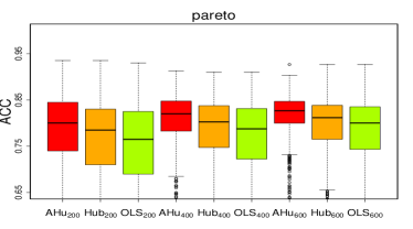
Figure 3 shows boxplots of the -norm of the estimation errors of the parameter with different errors and with , where the -norm is defined as , where is the robust estimator of the true parameter . Figure 4 shows boxplots of the accuracy (ACC) of subgroup identification with different errors and with . Here, ACC is defined as
with the robust estimator of the true parameter .
Figures 3 and 4 show that the -norms of the estimation errors decrease and the accuracies of subgroup identification increase as the sample size grows, which verifies the established theoretical results. Compared with the ordinary quadratic loss, the proposed estimation procedure achieves a uniformly lower median of the -norm of the estimation errors and higher accuracy of subgroup identification for all heavy-tailed distributions except for the distribution. The three methods are comparable for the symmetric distributions, such as the Gaussian and distributions. To limit the number of pages, the boxplots of the -norm of the estimation errors of the parameter and accuracy of subgroup identification for , and are shown in Figures E2–E4 and E6–E8 in Appendix E.1 of the Supplementary Material.


5 Case study
The proposed procedure is applied to cancer data for skin cutaneous melanoma (SKCM) downloaded from the Cancer Genome Atlas https://tcga-data.nci.nih.gov/. SKCM is one of the most aggressive types of cancer, and its incidence, mortality, and disease burden are increasing annually (Siegel et al., 2021; Xiong et al., 2019). It is believed that CREG1, TMEM201, and CCL8 are skin-cancer susceptibility genes (Hu et al., 2020), and the goal is to identify the subgroup of Breslow’s thickness based on mutations of those sensitive genes.
Consideration is given to the three environmental factors of (i) gender, (ii) age at diagnosis, and (iii) Clark level at diagnosis (CLAD), all of which have been studied extensively in the literature. Studies such as those by Dickson and Gershenwald, (2011) have found that these three environmental factors have positive effects. After removing missing values, there are 253 subjects, and the SKCM data are modeled by applying the change-plane model (1)
where , and . The three important genes CREG1, TMEM201, and CCL8 are high correlated with breast cancer (Hu et al., 2020).
Based on bootstrap samples and the Huber loss, the p-value with the proposed RWAST is , which implies that based on the proposed method, there is a strong evidence for rejecting the null hypothesis. However, based on the ordinary quadratic loss, the p-values with WAST and SST are 0.6454 and 0.0286, respectively, where and . Therefore, there is no evidence for rejecting the null hypothesis for WAST and SST based on the ordinary quadratic loss.
The parametric estimators are listed in Table 1, from which the indicator function partitions the population into two subgroups with 121 and 132 subjects based on the Huber loss, and two subgroups with 91 and 162 subjects based on the ordinary quadratic loss. Therefore, there would appear to be a subgroup with a higher chance of skin cancer based on mutations of these three genes CREG1, TMEM201, and CCL8.
| Change plane | Parameter | Intercept | AGE | GENDER | CLAD | Intercept | CREG1 | TMEM201 | CCL8 | |
|---|---|---|---|---|---|---|---|---|---|---|
| OLS | 0.002 | 0.050 | ||||||||
| 0.022 | 0.024 | 0.008 | ||||||||
| 1.000 | 0.179 | 4.970 | ||||||||
| Huber | 3.525 | 0.029 | 0.079 | 0.064 | ||||||
| 0.012 | 0.014 | |||||||||
| 1.000 | 0.384 | 4.860 |
6 Conclusion
Considered herein were subgroup classification and subgroup tests for change-plane models with heavy-tailed errors, which offer help in (i) narrowing down populations for modeling and (ii) providing recommendations for optimal individualized treatments in practice. A novel subgroup classifier was proposed by smoothing the indicator function and minimizing a smoothed Huber loss. Nonasymptotic properties were derived and nonasymptotic Bahadur representation was provided, in which the estimators of the parameters and achieve sub-Gaussian tails.
The novel test statistic RWAST was introduced to test whether subgroups of individuals exist. In a comparison with WAST Liu et al., (2024) and SST Andrews and Ploberger, (1994, 1995); Song et al., (2009); Fan et al., 2017a based on the ordinary change-plane regression with non-heavy-tailed errors, the proposed test statistic improved the power significantly because it is robust with the assistance of the Huber loss and avoids the drawbacks of taking the supremum over the parametric space when its dimension is large. Asymptotic distributions were derived under the null and alternative hypotheses. As studied by Liu et al., (2024) and Huang et al., (2020), it is easy to extend the proposed robust estimation procedure and RWAST to change-plane regression with multiple change planes with heavy-tailed errors.
In the age of big data, it is interesting to consider high-dimensional change-plane regression models and to provide high-dimensional robust estimation procedures and test statistics. As noted by Liu et al., (2024), the proposed RWAST can be applied to change-plane regression with high-dimensional grouping parameter . However, it remains open to provide estimation procedures for change-plane regression with high-dimensional . A possible strategy is to penalize the loss function with under the assumption of sparsity.
Supplementary Material
Appendix A includes Algorithm 1 for implementation in Section 2.3. Appendix B provides the computation of critical value in Section 3. Appendix C provides the proofs of Theorems 1–4 and the related Lemmas. Appendix D provides the proofs of Theorems 5–7. Appendix E provides additional simulation studies to illustrate the performance of the proposed estimation and test prcedures.
Acknowledgments
This work was supported in part by the NSFC (12271329, 72331005).
References
- Andrews and Ploberger, (1994) Andrews, D. W. K. and Ploberger, W. (1994). Optimal tests when a nuisance parameter is present only under the alternative. Econometrica, 62(6):1383–1414.
- Andrews and Ploberger, (1995) Andrews, D. W. K. and Ploberger, W. (1995). Admissibility of the Likelihood Ratio Test When a Nuisance Parameter is Present Only Under the Alternative. The Annals of Statistics, 23(5):1609 – 1629.
- Chen and Zhou, (2020) Chen, X. and Zhou, W.-X. (2020). Robust inference via multiplier bootstrap. The Annals of Statistics, 48(3):1665 – 1691.
- Davies, (1977) Davies, R. B. (1977). Hypothesis testing when a nuisance parameter is present only under the alternative. Biometrika, 64(2):247–254.
- Devroye et al., (2016) Devroye, L., Lerasle, M., Lugosi, G., and Oliveira, R. I. (2016). Sub-Gaussian mean estimators. The Annals of Statistics, 44(6):2695 – 2725.
- Dickson and Gershenwald, (2011) Dickson, P. V. and Gershenwald, J. E. (2011). Staging and prognosis of cutaneous melanoma. Surgical oncology clinics of North America, 20(1):1–17.
- (7) Fan, A., Rui, S., and Lu, W. (2017a). Change-plane analysis for subgroup detection and sample size calculation. Journal of the American Statistical Association, 112:769–778.
- (8) Fan, J., Li, Q., and Wang, Y. (2017b). Estimation of high dimensional mean regression in the absence of symmetry and light tail assumptions. Journal of the Royal Statistical Society: Series B (Statistical Methodology), 79(1):247–265.
- Foster et al., (2011) Foster, J. C., Taylor, J., and Ruberg, S. J. (2011). Subgroup identification from randomized clinical trial data. Statistics in Medicine, 30(24):2867–2880.
- Hahn et al., (1990) Hahn, M. G., Kuelbs, J., and Weiner, D. C. (1990). The Asymptotic Joint Distribution of Self-Normalized Censored Sums and Sums of Squares. The Annals of Probability, 18(3):1284 – 1341.
- Han et al., (2022) Han, D., Huang, J., Lin, Y., and Shen, G. (2022). Robust post-selection inference of high-dimensional mean regression with heavy-tailed asymmetric or heteroskedastic errors. Journal of Econometrics, 230(2):416 – 431.
- Horowitz, (1993) Horowitz, J. L. (1993). Optimal rates of convergence of parameter estimators in the binary response model with weak distributional assumptions. Econometric Theory, 9(1):1–18.
- Hu et al., (2020) Hu, B., Wei, Q., Zhou, C., Ju, M., Wang, L., Chen, L., Li, Z., Wei, M., He, M., and Zhao, L. (2020). Analysis of immune subtypes based on immunogenomic profiling identifies prognostic signature for cutaneous melanoma. International Immunopharmacology, 89:107162.
- Huang et al., (2020) Huang, Y., Cho, J., and Fong, Y. (2020). Threshold-based subgroup testing in logistic regression models in two-phase sampling designs. Applied Statistics, 70(2).
- Huber, (1964) Huber, P. J. (1964). Robust estimation of a location parameter. The Annals of Mathematical Statistics, 35(4):73–101.
- Huber, (1973) Huber, P. J. (1973). Robust Regression: Asymptotics, Conjectures and Monte Carlo. The Annals of Statistics, 1(5):799 – 821.
- Kang et al., (2024) Kang, C., Cho, H., Song, R., Banerjee, M., Laber, E. B., and Kosorok, M. R. (2024). Inference for change-plane regression. arXiv.org/abs/2206.06140.
- Kang et al., (2017) Kang, S., Lu, W., and Song, R. (2017). Subgroup detection and sample size calculation with proportional hazards regression for survival data. Statistics in Medicine, 36:4646 – 4659.
- Lee et al., (2011) Lee, S., Seo, M. H., and Shin, Y. (2011). Testing for threshold effects in regression models. Journal of the American Statistical Association, 106(493):220–231.
- Lepskii, (1992) Lepskii, O. V. (1992). Asymptotically minimax adaptive estimation. i: Upper bounds. optimally adaptive estimates. Theory of Probability & Its Applications, 36(4):682–697.
- Li et al., (2021) Li, J., Li, Y., Jin, B., and Kosorok, M. R. (2021). Multithreshold change plane model: Estimation theory and applications in subgroup identification. Statistics in Medicine, 40(15):3440–3459.
- Liu et al., (2024) Liu, X., Huang, J., Zhou, Y., Zhang, F., and Panpan, R. (2024). Efficient subgroup testing in change-planemodels. http://arxiv.org/abs/2408.00602.
- Mukherjee et al., (2020) Mukherjee, D., Banerjee, M., Mukherjee, D., and Ritov, Y. (2020). Asymptotic normality of a linear threshold estimator in fixed dimension with near-optimal rate. arXiv preprint arXiv:2001.06955.
- Mukherjee et al., (2022) Mukherjee, D., Banerjee, M., and Ritov, Y. (2022). On robust learning in the canonical change point problem under heavy tailed errors in finite and growing dimensions. Electronic Journal of Statistics, 16(1):1153 – 1252.
- Seo and Linton, (2007) Seo, M. H. and Linton, O. (2007). A smoothed least squares estimator for threshold regression models. Journal of Econometrics, 141(2):704–735.
- Shen and Qu, (2020) Shen, J. and Qu, A. (2020). Subgroup analysis based on structured mixedeffects models for longitudinal data. Journal of Biopharmaceutical Statistics, 30(4):607–622.
- Siegel et al., (2021) Siegel, R. L., Miller, K. D., Fuchs, H. E., and Jemal, A. (2021). Cancer statistics, 2021. CA: A Cancer Journal for Clinicians, 71(1):7–33.
- Song et al., (2009) Song, R., Kosorok, M. R., and Fine, J. P. (2009). On asymptotically optimal tests under loss of identifiability in semiparametric models. The Annals of Statistics, 37:2409 – 2444.
- Sun et al., (2020) Sun, Q., Zhou, W.-X., and Fan, J. (2020). Adaptive huber regression. Journal of the American Statistical Association, 115(529):254–265. PMID: 33139964.
- Wald, (1943) Wald, A. (1943). Tests of statistical hypotheses concerning several parameters when the number of observations is large. Transactions of the American Mathematical Society, 54(3):426–482.
- Wang et al., (2021) Wang, L., Zheng, C., Zhou, W., and Zhou, W.-X. (2021). A new principle for tuning-free huber regression. Statistica Sinica, 31:2153–2177.
- Wei and Kosorok, (2018) Wei, S. and Kosorok, M. R. (2018). The change-plane Cox model. Biometrika, 105(4):891–903.
- Xiong et al., (2019) Xiong, J., Bing, Z., and Guo, S. (2019). Observed survival interval: A supplement to tcga pan-cancer clinical data resource. Cancers, 11(3).
- Zhang et al., (2022) Zhang, Y., Wang, J. W., and Zhu, Z. (2022). Single-index thresholding in quantile regression. Journal of the American Statistical Association, 117(540):2222–2237.
- Zhou et al., (2018) Zhou, W.-X., Bose, K., Fan, J., and Liu, H. (2018). A new perspective on robust -estimation: Finite sample theory and applications to dependence-adjusted multiple testing. The Annals of Statistics, 46(5):1904 – 1931.