Robust Sequence Networked Submodular Maximization
Abstract
In this paper, we study the Robust optimization for sequence Networked submodular maximization (RoseNets) problem. We interweave the robust optimization with the sequence networked submodular maximization. The elements are connected by a directed acyclic graph and the objective function is not submodular on the elements but on the edges in the graph. Under such networked submodular scenario, the impact of removing an element from a sequence depends both on its position in the sequence and in the network. This makes the existing robust algorithms inapplicable. In this paper, we take the first step to study the RoseNets problem. We design a robust greedy algorithm, which is robust against the removal of an arbitrary subset of the selected elements. The approximation ratio of the algorithm depends both on the number of the removed elements and the network topology. We further conduct experiments on real applications of recommendation and link prediction. The experimental results demonstrate the effectiveness of the proposed algorithm.
Introduction
Submodularity is an important property that models a diminishing return phenomenon, i.e., the marginal value of adding an element to a set decreases as the set expands. It has been extensively studied in the literature, mainly accompanied with maximization or minimization problems of set functions (Nemhauser and Wolsey 1978; Khuller, Moss, and Naor 1999). This is called submodularity. Mathematically, a set function is submodular if for any two sets and an element , we have . Such property finds a wide range of applications in machine learning, combinatorial optimization, economics, and so on. (Krause 2005; Lin and Bilmes 2011; Li et al. 2022; Shi et al. 2021; Kirchhoff and Bilmes 2014; Gabillon et al. 2013; Kempe, Kleinberg, and Tardos 2003; Wang et al. 2021).
Further equipped with monotonicity, i.e., for any , a submodular set function can be maximized by the cardinality constrained classic greedy algorithm, achieving an approximation ratio up to (Nemhauser and Wolsey 1978) (almost the best). Since then, the study of submodular functions has been extended by a variety of different scenarios, such as non-monotone scenario, adaptive scenario, and continuous scenario, etc (Feige, Mirrokni, and Vondrak 2007; Golovin and Krause 2011; Das and Kempe 2011; Bach 2019; Shi et al. 2019).
The above works focus on the set functions. In real applications, the order of adding elements plays an important role and affects the function value significantly. Recently, the submodularity has been generalized to sequence functions (Zhang et al. 2015; Tschiatschek, Singla, and Krause 2017; Streeter and Golovin 2008; Zhang et al. 2013). Considering sequences instead of sets causes an exponential increase in the size of the search space, while allowing for much more expressive models.
In this paper, we consider that the elements are networked by a directed graph. The edges encode the additional value when the connected elements are selected in a particular order. Such setting is not given a specific name before. To distinguish from the classic submodularity, we in this paper name it as networked submodularity (Net-submodularity for short). More specifically, the Net-submodular function is a sequence function, which is not submodular on the induced element set by but is submodular on the induced edge set by . The Net-submodularity is first considered in (Tschiatschek, Singla, and Krause 2017), which mainly focuses on the case where the underlying graph is a directed acyclic graph. General graphs and hypergraphs are considered in (Mitrovic et al. 2018).
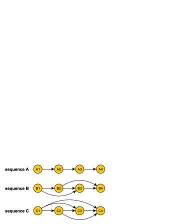
Recently, robust versions of the submodular maximization problem have arisen (Orlin, Schulz, and Udwani 2018; Mitrovic et al. 2017; Bogunovic et al. 2017; Sallam et al. 2020) to meet the increasing demand in the stability of the system. The robustness of the model mainly concerns with its ability in handling the malfunctions or adversarial attacks, i.e., the removal of a subset of elements in the selected set or sequence. Sample cases of elements removal in real world scenarios include items sold out or stop production in recommendation (Mitrovic et al. 2018), web failure of user logout in link prediction (Mitrovic et al. 2019) and equipment malfunction in sensor allocation or activation (Zhang et al. 2015). In this paper, we take one step further and study a new problem of robust sequence networked submodular maximization (RoseNets). We show an example in Figure 1 to illustrate the importance of RoseNets problem.
See in Figure 1. Suppose all edge weights in sequence A are 0.9, in sequence B are 0.5, in sequence C are 0.4. Let the net-submodular utility function of the sequence be the summation of all the weights of the induced edge set by the sequence. Such utility function is obviously monotone but not submodular.111Easy to see that in sequence B, the utility of is 0, but is 0.5, which violates the submodularity. However, it is submodular on the edge set. Now we can see, the utility of sequence A, B and C are 2.7 (largest), 2.5 and 2.4 respectively. We can easily check that if one node would be removed in each sequence, the worst utility after removal of sequence A, B and C is 0.9, 1.0 (largest), and 0.8. If we remove two nodes in each sequence, the utility of A, B and C becomes 0, 0, and 0.4 (largest). With different number of nodes removed, the three sequences show different robustness. Existing non-robust algorithm may select sequence A since it has the largest utility. However, sequence B and C are more robust against node removal.
Given a net-submodular function and the corresponding network, the RoseNets problem aims to select a sequence of elements with cardinality constraints, such that the value of the sequence function is maximized when a certain number of the selected elements may be removed. As far as sequence functions and net-submodularity are concerned, the design and analysis of robust algorithms are faced with novel technical difficulties. The impact of removing an element from a sequence depends both on its position in the sequence and in the network. This makes the existing robust algorithms inapplicable here. It is unclear what conditions are sufficient for designing efficient robust algorithm with provable approximation ratios for RoseNets problem. We aim to take a step for answering this question in this paper. Our contributions are summarized as follows.
-
1.
To the best of our knowledge, this is the first work that considers the RoseNets problem. Combining robust optimization and sequence net-submodular maximization requires subtle yet critical theoretical efforts.
-
2.
We design a robust greedy algorithm that is robust against the removal of an arbitrary subset of the selected sequence. The theoretical approximation ratio depends both on the number of the removed elements and the network topology.
-
3.
We conduct experiments on real applications of recommendation and link prediction. The experimental results demonstrate the effectiveness and robustness of the proposed algorithm, against existing sequence submodular baselines. We hope that this work serves as an important first step towards the design and analysis of efficient algorithms for robust submodular optimization.
Related Works
Submodular maximization has been extensively studied in the literature. Efficient approximation algorithms have been developed for maximizing a submodular set function in various settings (Nemhauser and Wolsey 1978; Khuller, Moss, and Naor 1999; Calinescu et al. 2011; Chekuri, Vondrák, and Zenklusen 2014). By considering the robustness requirement, recently, robust versions of submodular maximization have been extensively studied. These works aim at selecting a set of elements that is robust against the removal of a subset of elements. The first algorithm for the cardinality constrained robust submodular maximization problem is studied in (Orlin, Schulz, and Udwani 2018). A constant factored approximation ratio is achieved. The selected -sized set is robust against the removal of any elements of the selected set. The constant approximation ratio is valid as long as . An improvement is made in (Bogunovic et al. 2017), which provide an algorithm that guarantees the same constant approximation ratio but allows the removal of a larger number of elements (i.e.,. With a mild assumption, the algorithm proposed in (Mitrovic et al. 2017) allows the removal of an arbitrary number of elements. The restriction on is relaxed in (Tzoumas et al. 2017), while the derived approximation ratio is parameterized . This work is extended to a multi-stage setting in (Tzoumas, Jadbabaie, and Pappas 2018) and (Tzoumas, Jadbabaie, and Pappas 2020). The decision at each stage would takes into account the failures that happened in the previous stages. Other constrains that are combined with the robust optimization include fairness, privacy issues and so on (Mirzasoleiman, Karbasi, and Krause 2017; Kazemi, Zadimoghaddam, and Karbasi 2018).
The concept of sequence (or string) submodularity for sequence functions is a generalization of submodularity, which has been introduced recently in several studies (Zhang et al. 2015; Streeter and Golovin 2008; Zhang et al. 2013) The above works all consider element-based robust submodular maximization. Networked submodularity is considered in (Tschiatschek, Singla, and Krause 2017; Mitrovic et al. 2018), where the sequential relationship among elements is encoded by a directed acyclic graph. Following the networked submodularity setting, the work in (Mitrovic et al. 2019) introduces the idea of adaptive sequence submodular maximization, which aims to utilize the feedback obtained in previous iterations to improve the current decision. In this paper, we follow the networked submodularity setting, and study the RoseNets problem. It is unclear whether all of the above algorithms can be properly extended to our problem, as converting a set function to a sequence function and submodularity to networked submodularity could result in an arbitrarily bad performance. Establishing the approximation guarantees for RoseNets problem would require a more sophisticated analysis, which calls for more in-depth theoretical efforts.
System Model and Problem Definition
In this paper, we follow the networked submodular sequence setting (Tschiatschek, Singla, and Krause 2017; Mitrovic et al. 2018). Let be the set of elements. A set of edges represents that there is additional utility in picking certain elements in a certain order. More specifically, an edge represents that there is additional utility in selecting after has already been chosen. Self-loops (i.e., edges that begin and end at the same element) represents that there is individual utility in selecting an element.
Given a directed graph , a non-negative monotone submodular set function , and a parameter , the objective is to select a non-repeating sequence of unique elements that maximizes the objective function:
where contains all the edges that is select before in .
We say is the set of edges induced by the sequence . It is important to note that the function is a submodular set function over the edges, not over the elements. Furthermore, the objective function is neither a set function, nor is it necessarily submodular on the elements. We call such a function as a networked submodular function.
We define to represent the residual value of the objective function after the removal of elements in set . In this paper, the robust sequence networked submodular maximization (RoseNets) problem is formally defined below.
Definition 1.
Given a directed graph , a networked submodular function and robustness parameter , the RoseNets problem aims at finding a sequence such that it is robust against the worst possible removal of nodes:
The robustness parameter represents the size of the subset that is removed. After the removal, the objective value should remain as large as possible. For , the problem reduces to the classic sequence submodular maximization problem (Mitrovic et al. 2018).
Robust Algorithm and Theoretical Results
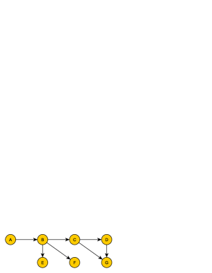
Direct applying the Sequence Greedy algorithm (Mitrovic et al. 2018) to solve the RoseNets problem would return an arbitrary bad solution. We can construct a very simple example for an illustration. See in Figure 2. Let the edge weights of be 0.9 and be 0.5. Let the net-submodular utility function of the selected sequence be the summation of all weights of the induced edge set by the sequence. Suppose we are to select a sequence with 5 elements. Using the Sequence Greedy algorithm, sequence will be selected222Suppose elements are selected in the alphabetic order if the edge weights are equal. Similar examples can be easily constructed when elements are selected at random. for maximizing the utility, i.e., . However, if , i.e., two elements would be removed, removing and any other one element (worst case) makes the utility become 0.
RoseNets Algorithm
We wish to design an algorithm that is robust against the removal of an arbitrary subset of selected elements. In this paper, we propose the RoseNets Algorithm, which can approximately solves the RoseNets problem and is shown in Algorithm 1. Note we consider the case that .
The limitation of the Sequence Greedy algorithm is that the selected sequence is vulnerable. The overall utility might be concentrated in the first few elements. Algorithm 1 is motivated by this key observation and works in two steps. In Step 1 (the first while loop), we select a sequence of elements from in a greedy manner as in Sequence Greedy. In Step 2 (the second while loop), we select another sequence of elements from , again in a greedy manner as in Sequence Greedy. Note that when we select sequence , we perform the greedy selection as if sequence does not exist at all. This ensures that the value of the final returned sequence is not concentrated in either or . The complexity of Algorithm 1 is , which is in terms of the number of function evaluations used in the algorithm.
To show the differences and benefits of the RoseNets algorithm, we go back to see the example in Figure 2. When and , the RoseNets algorithm will select the sequence and sequence . When selecting , the RoseNets algorithm would not consider element in . Thus element and are regarded as making not contribution to the utility function. The RoseNets algorithm will return the sequence . The worst case of removing elements, is to remove and any one element in . The residual utility is 0.5. Remember the case for Sequence Greedy algorithm, the residual utility of the worst case is 0. This example shows the benefits of the RoseNets algorithm.
Both the examples in Figure 1 and Figure 2 imply that a robust sequence should have complex network structure. The utility should not concentrate in a center element, but aggregated from all the edges among elements in the sequence. Such a robust sequence can only be selected by multiple trials of greedy selection, with the trials neglecting each other. Otherwise, the central element (if exists) with its high edge weight neighbors are probability selected, as node in Figure 2. If such a node is removed, the utility would slump. In this paper, we implement such intuitive strategy by using two trials of greedy selection. Intuitively, invoking more times of greedy selection trial may improve the approximation ratio. However, as we are to take a first step in the RoseNets problem while our theoretical analysis is already non-trivial, we leave the design of multi-part selection algorithm and the approximation ratio analysis for future works.
Theoretical Results
Let , , , . Note and are the maximum in and out degree of the network respectively. For convience, we denote and as the marginal gain of attending and to sequence respectively. We denote as the optimal solution of the RoseNets problem with element set , cardinality and robust parameter , and be the minimum value of after elements are removed from .
Theorem 1.
Consider , Algorithm 1 achieves an approximation ratio of
Theorem 2.
Consider , Algorithm 1 achieves an approximation ratio of
In Theorem 1, it is hard to compare the two approximation ratios directly due to their complex mathematical expression. Thus we consider specific network setting to show the different advantages of the two terms.
First, it is easy to verify that both the two terms are monotonically increasing function of . When , we have . Thus we know that when is small, the first term is larger. When , the first term has a limit value of , and the second term has a limit value of .When , then and . In this case, the second term is larger than the first term in Theorem 1. Thus we can conclude that under specific network structure, the second term would be larger with large .
Similarly, for Theorem 2, when and , . Thus we know when and is small, the first term is larger. When while remains a constant, the first term has a limit value of , the second term has a limit value of . When and , then , and . In this case, the second term is larger than the first term in Theorem 2. Thus we can conclude that under specific network structure, the second term would be larger with large .
According to the above analysis, we know that the value of and , together with the network topology, significantly affect the approximation ratio. It would be an interesting future direction to explore how the approximation ratio change when the parameters and network topology change.
To prove the above two theorems, we need the following three auxiliary lemmas. Due to space limitations, we here assume Lemma 1, 2 and 3 hold and show the proof of Theorem 1 below. We provide the proofs of Lemma 1, 2, 3 and Theorem 2 in the supplementary material.
Lemma 1.
There exists an element for sequence and satisfies that .
Lemma 2.
Consider and . Suppose that the sequence selected is with and that there exists a sequence with such that and . Then we have .
Lemma 3.
Consider . The following holds for any with : .
Proof of Theorem 1
Given , the selected sequence has one element. And we have . Let . Then the final sequence is . Suppose the the removed vertex from the sequence is .
First, we show a lower bound on :
| (1) | ||||
The first inequality is due to the approximation ratio of Sequence Greedy algorithm for net-submodular maximization (Mitrovic et al. 2018). The second inequality is due to Lemma 3.
Now, we can see the removed element can be either or an element in . In the following, we will consider these two cases:
Case 1. Let . Then we have
| (2) |
Case 2. Let . We then further consider two cases:
Case 2.1. Let .
In this case, the removal does not reduce the overall value of the remaining sequence . Then we have
| (3) | ||||
Case 2.2. Let .
We define , to represent the ratio of the loss of removing element from sequence to the value of the sequence . Obviously, we have since .
First, we have
| (4) | ||||
where / are the edge that has maximum utility over all the incoming/outgoing edges of . The first inequality is due to the fact that the marginal gain of a vertex to the prefix and subsequent sequence is at most and . Then the second inequality follows intuitively.
Given Equation (4), we need to prove four inequalities for finally proving the theorem.
First, suppose the first vertex of is . By the monotonicity of function and Equation (4), we have
| (5) | ||||
Given Equation (5), we have Inequality 1 as below.
Inequality 1:
We know for and .333As is monotone increasing and is monotone decreasing, the function achieves the maximum value when Thus we have Inequality 2 as below.
Inequality 2:
Note that the first two elements in satisfy that
Thus by replacing the parameters in Lemma 2 and Lemma 3, we have the following result, which implies Inequality 3.
Now define and . It is easy to verify that for and , / is monotonically increasing/decreasing. Note when , . We consider two cases for : (1) when , we have as is monotonically decreasing; (2) when , we have as is monotonically increasing. Thus we have the Inequality 4 as below.
Inequality 4:
Combining Inequality 1, Inequality 2 and Equation (1), we can have the first lower bound in Theorem 1:
Combining Inequality 1, Inequality 3 and Inequality 4, we can have the second lower bound in Theorem 1:
Now we are done.
Experiments
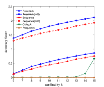
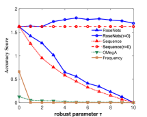
We compare the performance of our algorithms RoseNets to the non-robust version Sequence Greedy (Sequence for short) (Mitrovic et al. 2018), the existing submodular sequence baseline (OMegA) (Tschiatschek, Singla, and Krause 2017), and a naive baseline (Frequency) which outputs the most popular items the user has not yet reviewed.
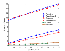
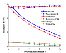
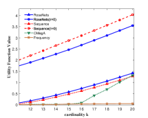
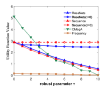
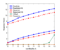
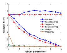
To evaluate the performance of the algorithms, we use three evaluation metrics in this paper. The first one is Accuracy Score, which simply counts the number of accurately recommended items. While this is a sensible measure, it does not explicitly consider the order of the sequence. Therefore, we also consider the Sequence Score, which is a measure based on the Kendall-Tau distance (Kendall 1938). This metric counts the number of ordered pairs that appear in both the predicted sequence and the true sequence. These two metrics are also used in (Mitrovic et al. 2019). The third metric is the Utility Function Value of the selected sequence.
We use a probabilistic coverage utility function as our Net-submodular function . Mathematically,
where is the edges induced by sequence . And to simulate the worst case removal, we remove the first elements to evaluate the robustness of the algorithms.
Amazon Product Recommendation
Using the Amazon Video Games review dataset (Ni, Li, and McAuley 2019), we conduct experiments for the task of recommending products to users. In particular, given a specific user with the first 4 products she has purchased, we want to predict the next products she will buy. We first build a graph , where is the set of all products and is the set of edges between these products. The weight of each edge, , is defined to be the conditional probability of purchasing product given that the user has previously purchased product . We compute by taking the fraction of users that purchased after having purchased among all the users that purchased . There are also self-loops with weight that represent the fraction of users that purchased product among all the users. We focused on the products that have been purchased at least 50 times each, leaving us with a total of 9383 unique products. Also we select the users that have purchased at least 29 products, leaving use 909 users. We conduct recommendation task on these 909 users and take the average value of each evaluation metric.
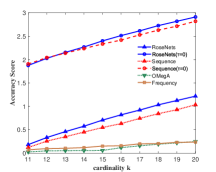
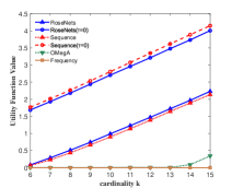
Figure 3 shows the performance of the comparison algorithms using the accuracy score, sequence score and utility function value respectively. In Figure 3(a), 3(b), 3(c) and 3(d), we find that after the removal of elements, the RoseNets outperforms all the comparisons. Such results demonstrate that the RoseNets algorithm is effective and robust in real applications since accuracy score and sequence score are common evaluation metrics in practical. In Figure 3(e) and 3(f), the only difference is that the OMegA algorithm is outperforming when is small or is large. The OMegA algorithm aims to find a global optimal solution. It topologically resorts all the candidates after each element selection. It can return a solution with better utility function value when is large and is small, but runs much slower than RoseNets or Sequence. Also, it shows poor performance in accuracy and sequence score. Thus the RoseNets algorithm is more effective and robust in real applications.
In addition, we also show the case of RoseNets and Sequence with . We can see that in all the experimental results for the three metrics, the RoseNets outperforms Sequence, which is consistent to our expectation. On utility function value, the Sequence() is better than the RoseNets(). However, on accuracy score and sequence score, the RoseNets() is very close to the Sequence(), sometimes shows better performance. The former result is due to the effectiveness of greedy framework. The RoseNets algorithm indeed invokes Sequence for two trials independently, which intuitively cannot achieve comparable performance with one trial Sequence execution, due to the Net-submodularity. But the latter result shows that directly implementing greedy selection is not always outperforming. This is due to the intrinsic property of the greedy algorithm. Though is almost the best approximation ratio, some heuristic algorithms may achieve better performance in specific cases. However, if we invoke more trials of Sequence algorithm, better robust experimental results and approximation ratio might be achieved but the utility value would become lower. This is because more trials of independent greedy selection would give high probability of triggering the diminishing return phenomenon. In real applications, this is a trade-off for designing robust algorithms that requires a balance between high efficiency on robustness and maximization of utility value.
Wikipedia Link Prediction
Using the Wikispeedia dataset (West, Pineau, and Precup 2009), we consider users who are surfing through Wikipedia towards some target article. Given a sequence of articles the user has previously visited, we want to guide her to the page she is trying to reach. Since different pages have different valid links, the order of pages we visit is critical to this task. Formally, given the first 4 pages each user visited, we want to predict which page she is trying to reach by making a series of suggestions for which link to follow. In this case, we build the graph , where is the set of all pages and is the set of existing links between pages. Similarly to the recommendation case, the weight of an edge is the probability of moving to page given that the user is currently at page , i.e., the fraction of moves from to among all the visit of . In this case, we build no self-loops as we assume we can only move using links. Thus we cannot jump to random pages. We condense the dataset to include only articles and edges that appeared in a path, leaving us 4170 unique pages and 55147 edges. We run the algorithm on paths with length at least 29, which leaves us 271 paths. We conduct link prediction task on these 271 paths and take the average value of each evaluation metric.
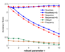
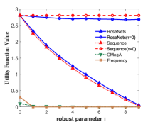
Figure 4 shows the performance of the comparison algorithms using the accuracy score, sequence score and utility function value respectively. In Figure 4, we find that after the removal of elements, the RoseNets outperforms all the comparisons in all the cases. These results demonstrate that the RoseNets algorithm is effective and robust in real applications. The OMegA algorithm does not show comparable performance to RoseNets algorithm any more. This is because that (1) the path need to be predicted is very long, and (2) the intersection part of different paths is not as large as the case in Amazon recommendation experiments. Thus the global algorithm OMegA cannot exploit its advantages. We still can find in Figure 4(a), 4(c) and 4(e) that when becomes larger, the performance of OMegA algorithm increases faster. This in turn demonstrates that the RoseNets algorithm is more general, effective and robust, which does not assume specific real application scenario.
Another difference in the link prediction application is that, the RoseNets() outperforms Sequence() almost in all the cases on accuracy and sequence score. This again verifies that directly implementing greedy selection may sometimes far away from the optimal solution. As discussed in the end of the recommendation case, an interesting future direction is to explore the trade-off between high efficiency on robustness and the maximization of utility value by invoking more independent greedy selection trials.
Conclusion
In this paper, we are the first to study the RoseNets problem, which combines the robust optimization and sequence networked submodular maximization. We design a robust algorithm with an approximation ratio that is bounded by the number of the removed elements and the network topology. Experiments on real applications of recommendation and link prediction demonstrate the effectiveness of the proposed algorithm. For future works, one direction is to develop robust algorithms that can achieve higher approximation ratio. An intuitive improvement is to invoke multiple trials of independent greedy selection. Another direction is to consider the robustness against the removal of edges. This is non-trivial since different removal operation would change the network topology and affect the approximation ratio.
Acknowledgments
This work is supported by the National Natural Science Foundation of China (Grant No: 62102357, U1866602, 62106221, 62102382), and the Starry Night Science Fund of Zhejiang University Shanghai Institute for Advanced Study (Grant No: SN-ZJU-SIAS-001). It is also partially supported by the Zhejiang Provincial Key Research and Development Program of China (2021C01164).
References
- Bach (2019) Bach, F. 2019. Submodular functions: from discrete to continuous domains. Mathematical Programming, 175(1): 419–459.
- Bogunovic et al. (2017) Bogunovic, I.; Mitrović, S.; Scarlett, J.; and Cevher, V. 2017. Robust submodular maximization: A non-uniform partitioning approach. In International Conference on Machine Learning, 508–516. PMLR.
- Calinescu et al. (2011) Calinescu, G.; Chekuri, C.; Pal, M.; and Vondrák, J. 2011. Maximizing a monotone submodular function subject to a matroid constraint. SIAM Journal on Computing, 40(6): 1740–1766.
- Chekuri, Vondrák, and Zenklusen (2014) Chekuri, C.; Vondrák, J.; and Zenklusen, R. 2014. Submodular function maximization via the multilinear relaxation and contention resolution schemes. SIAM Journal on Computing, 43(6): 1831–1879.
- Das and Kempe (2011) Das, A.; and Kempe, D. 2011. Submodular meets spectral: greedy algorithms for subset selection, sparse approximation and dictionary selection. In Proceedings of the 28th International Conference on International Conference on Machine Learning, 1057–1064.
- Feige, Mirrokni, and Vondrak (2007) Feige, U.; Mirrokni, V. S.; and Vondrak, J. 2007. Maximizing Non-Monotone Submodular Functions. In Proceedings of the 48th Annual IEEE Symposium on Foundations of Computer Science, 461–471.
- Gabillon et al. (2013) Gabillon, V.; Kveton, B.; Wen, Z.; Eriksson, B.; and Muthukrishnan, S. 2013. Adaptive submodular maximization in bandit setting. Advances in Neural Information Processing Systems, 26.
- Golovin and Krause (2011) Golovin, D.; and Krause, A. 2011. Adaptive submodularity: Theory and applications in active learning and stochastic optimization. Journal of Artificial Intelligence Research, 42: 427–486.
- Kazemi, Zadimoghaddam, and Karbasi (2018) Kazemi, E.; Zadimoghaddam, M.; and Karbasi, A. 2018. Scalable deletion-robust submodular maximization: Data summarization with privacy and fairness constraints. In International conference on machine learning, 2544–2553. PMLR.
- Kempe, Kleinberg, and Tardos (2003) Kempe, D.; Kleinberg, J.; and Tardos, É. 2003. Maximizing the spread of influence through a social network. In Proceedings of the ninth ACM SIGKDD international conference on Knowledge discovery and data mining, 137–146. ACM.
- Kendall (1938) Kendall, M. G. 1938. A new measure of rank correlation. Biometrika, 30(1/2): 81–93.
- Khuller, Moss, and Naor (1999) Khuller, S.; Moss, A.; and Naor, J. S. 1999. The budgeted maximum coverage problem. Information processing letters, 70(1): 39–45.
- Kirchhoff and Bilmes (2014) Kirchhoff, K.; and Bilmes, J. 2014. Submodularity for data selection in machine translation. In Proceedings of the 2014 Conference on Empirical Methods in Natural Language Processing (EMNLP), 131–141.
- Krause (2005) Krause, A. 2005. Near-optimal nonmyopic value of information in graphical models. In Proc. of the 21st Annual Conf. on Uncertainty in Artificial Intelligence (UAI 2005), 324–331.
- Li et al. (2022) Li, M.; Wang, T.; Zhang, H.; Zhang, S.; Zhao, Z.; Zhang, W.; Miao, J.; Pu, S.; and Wu, F. 2022. HERO: HiErarchical spatio-tempoRal reasOning with Contrastive Action Correspondence for End-to-End Video Object Grounding. In ACM MM.
- Lin and Bilmes (2011) Lin, H.; and Bilmes, J. 2011. A class of submodular functions for document summarization. In Proceedings of the 49th annual meeting of the association for computational linguistics: human language technologies, 510–520.
- Mirzasoleiman, Karbasi, and Krause (2017) Mirzasoleiman, B.; Karbasi, A.; and Krause, A. 2017. Deletion-robust submodular maximization: Data summarization with “the right to be forgotten”. In International Conference on Machine Learning, 2449–2458. PMLR.
- Mitrovic et al. (2018) Mitrovic, M.; Feldman, M.; Krause, A.; and Karbasi, A. 2018. Submodularity on hypergraphs: From sets to sequences. In International Conference on Artificial Intelligence and Statistics, 1177–1184. PMLR.
- Mitrovic et al. (2019) Mitrovic, M.; Kazemi, E.; Feldman, M.; Krause, A.; and Karbasi, A. 2019. Adaptive sequence submodularity. Advances in Neural Information Processing Systems, 32.
- Mitrovic et al. (2017) Mitrovic, S.; Bogunovic, I.; Norouzi-Fard, A.; Tarnawski, J. M.; and Cevher, V. 2017. Streaming robust submodular maximization: A partitioned thresholding approach. Advances in Neural Information Processing Systems, 30.
- Nemhauser and Wolsey (1978) Nemhauser, G. L.; and Wolsey, L. A. 1978. Best algorithms for approximating the maximum of a submodular set function. Mathematics of operations research, 3(3): 177–188.
- Ni, Li, and McAuley (2019) Ni, J.; Li, J.; and McAuley, J. 2019. Justifying recommendations using distantly-labeled reviews and fine-grained aspects. In Proceedings of the 2019 conference on empirical methods in natural language processing and the 9th international joint conference on natural language processing (EMNLP-IJCNLP), 188–197.
- Orlin, Schulz, and Udwani (2018) Orlin, J. B.; Schulz, A. S.; and Udwani, R. 2018. Robust monotone submodular function maximization. Mathematical Programming, 172(1): 505–537.
- Sallam et al. (2020) Sallam, G.; Zheng, Z.; Wu, J.; and Ji, B. 2020. Robust sequence submodular maximization. Advances in Neural Information Processing Systems, 33: 15417–15426.
- Shi et al. (2019) Shi, Q.; Wang, C.; Ye, D.; Chen, J.; Feng, Y.; and Chen, C. 2019. Adaptive influence blocking: Minimizing the negative spread by observation-based policies. In 2019 IEEE 35th international conference on data engineering (ICDE), 1502–1513. IEEE.
- Shi et al. (2021) Shi, Q.; Wang, C.; Ye, D.; Chen, J.; Zhou, S.; Feng, Y.; Chen, C.; and Huang, Y. 2021. Profit maximization for competitive social advertising. Theoretical Computer Science, 868: 12–29.
- Streeter and Golovin (2008) Streeter, M.; and Golovin, D. 2008. An online algorithm for maximizing submodular functions. Advances in Neural Information Processing Systems, 21.
- Tschiatschek, Singla, and Krause (2017) Tschiatschek, S.; Singla, A.; and Krause, A. 2017. Selecting sequences of items via submodular maximization. In Thirty-First AAAI Conference on Artificial Intelligence.
- Tzoumas et al. (2017) Tzoumas, V.; Gatsis, K.; Jadbabaie, A.; and Pappas, G. J. 2017. Resilient monotone submodular function maximization. In 2017 IEEE 56th Annual Conference on Decision and Control (CDC), 1362–1367. IEEE.
- Tzoumas, Jadbabaie, and Pappas (2018) Tzoumas, V.; Jadbabaie, A.; and Pappas, G. J. 2018. Resilient monotone sequential maximization. In 2018 IEEE Conference on Decision and Control (CDC), 7261–7268. IEEE.
- Tzoumas, Jadbabaie, and Pappas (2020) Tzoumas, V.; Jadbabaie, A.; and Pappas, G. J. 2020. Robust and adaptive sequential submodular optimization. IEEE Transactions on Automatic Control.
- Wang et al. (2021) Wang, C.; Shi, Q.; Xian, W.; Feng, Y.; and Chen, C. 2021. Efficient diversified influence maximization with adaptive policies. Knowledge-Based Systems, 213: 106692.
- West, Pineau, and Precup (2009) West, R.; Pineau, J.; and Precup, D. 2009. Wikispeedia: An online game for inferring semantic distances between concepts. In Twenty-First IJCAI.
- Zhang et al. (2015) Zhang, Z.; Chong, E. K.; Pezeshki, A.; and Moran, W. 2015. String submodular functions with curvature constraints. IEEE Transactions on Automatic Control, 61(3): 601–616.
- Zhang et al. (2013) Zhang, Z.; Wang, Z.; Chong, E. K.; Pezeshki, A.; and Moran, W. 2013. Near optimality of greedy strategies for string submodular functions with forward and backward curvature constraints. In 52nd IEEE Conference on Decision and Control, 5156–5161. IEEE.
Appendices: Omitted Proofs
Proof of Lemma 1
Lemma 1. There exists a vertex for sequence and satisfies that .
Proof.
Define and . We denote as the th to th elements in .
There must exist an index such that
Due to the submodularity of , we have
Thus there exists some element and some vertex such that
∎
Proof of Lemma 2
Lemma 2. Consider and . Suppose that the sequence selected by the Sequence Greedy Algorithm is with and that there exists a sequence with such that and . Then we have .
Proof.
Let be the -th vertex of sequence . Let be the sequence consisting of the first vertices of sequence . We can safely assume that .
where is the edge that selected by the algorithm making added into the returned sequence. The above inequalities hold due to the fact that the function is monotone, Sequence Greedy algorithm select the edge of largest marginal value each time, and adding to may add at most edges.
Rewriting the above inequality, we have
Writing for , we have
Thus we have
Suppose for some . Then we have
Then we have
∎
Proof of Lemma 3
Lemma 3. Consider . The following holds for any with : .
Proof.
Let be the set that minimizes . We can safely assume .
Let and . Obviously, . Also, we have
Thus the set is a feasible solution to minimize function with and . Thus we have
In addition, we have . This implies that
The elements in are not in . Thus we have
Note the sequence does not contain any element in and has elements. It is a feasible solution to minimize function with and . Thus we have
Also we have
Hence we proved . ∎
Proof of Theorem 2
Theorem 2. Consider , Algorithm 1 achieves an approximation ratio of
Proof.
After the execution of the RoseNets Algorithm, the selected sequence where and . Define as the removed set of vertices that can minimize , where and . First, we have a lower bound for :
The proof of Theorem 2 follows a similar line of the proof of Theorem 1. Specifically, we consider two cases as follows:
Case 1. , which means that all the removed vertices are in . Thus we have
Case 2. . In this case, we further consider two cases.
Case 2.1. Let .
In this case, the removal of elements in does not reduce the overall value of the remaining sequence. Then we have
Case 2.2. Let . Let and . Then we have and .
Let , denote the ratio of the loss of removing elements in from sequence to the value of the sequence . We have since .
Let the elements in be denoted by according to their order in sequence . Then we can rewrite as , where is the subsequence between item and , for and and are empty sequences. Note can be an empty sequence for any . Then we have
where / is the maximum in/out degree of the network, / are the edge that has maximum utility over all the incoming/outgoing edges of all the removed nodes . The first inequality is due to the fact that the marginal gain of a vertex to the prefix and subsequent sequence is at most and . Then the second inequality follows intuitively.
Given Equation (4), we need to prove four inequalities for finally proving the theorem.
First, suppose the first vertex of is . By the monotonicity of function and the above inequality, we have
Then we have Inequality 1 as below.
Inequality 1:
By similar analysis in the proof of Theorem 1, we have inequality 2 as below.
Inequality 2:
Let be the sequence consisting of the first elements of sequence . Then we have
Thus we have
Now define and . It is easy to verify that for and , / is monotonically increasing/decreasing. Note when , . We consider two cases for : (1) when , we have as is monotonically decreasing; (2) when , we have as is monotonically increasing. Thus we have the Inequality 4 as below.
Inequality 4:
Combining Inequality 1, Inequality 2 and the lower bound of , we can have the first lower bound in Theorem 2:
Combining Inequality 1, Inequality 3 and Equation Inequality 4, we can have the second lower bound in Theorem 2:
Since , the theorem holds. ∎