Robust Power Allocation for Integrated Visible Light Positioning and Communication Networks
Abstract
Integrated visible light positioning and communication (VLPC), capable of combining advantages of visible light communications (VLC) and visible light positioning (VLP), is a promising key technology for the future Internet of Things. In VLPC networks, positioning and communications are inherently coupled, which has not been sufficiently explored in the literature. We propose a robust power allocation scheme for integrated VLPC Networks by exploiting the intrinsic relationship between positioning and communications. Specifically, we derive explicit relationships between random positioning errors, following both a Gaussian distribution and an arbitrary distribution, and channel state information errors. Then, we minimize the Cramer-Rao lower bound (CRLB) of positioning errors, subject to the rate outage constraint and the power constraints, which is a chance-constrained optimization problem and generally computationally intractable. To circumvent the nonconvex challenge, we conservatively transform the chance constraints to deterministic forms by using the Bernstein-type inequality and the conditional value-at-risk for the Gaussian and arbitrary distributed positioning errors, respectively, and then approximate them as convex semidefinite programs. Finally, simulation results verify the robustness and effectiveness of our proposed integrated VLPC design schemes.
Index Terms:
Visible light communication, Visible light positioning, Robust power allocation, Outage probability.I INTRODUCTION
As predicted by Cisco, over billion Internet of Things (IoT) devices will be connected to the Internet globally by 2030, and about of the mobile traffic occurs in indoor environments[1]. This would also lead to growing demands for indoor location-based services, which are supported by accurate positioning and high data rates[2, 3]. The related applications include smart manufacturing, safety monitoring, logistics management, and indoor navigation. For indoor environments, the global navigation satellite system (GNSS) signals are usually weak due to the multipath effect and signal blocking. Meanwhile, conventional radio frequency (RF) based indoor positioning approaches, e.g., Wi-Fi, radio frequency identification (RFID), and ultra-wideband (UWB), generally suffer from electromagnetic interference, sensitivity to the changing environment, and multipath effects. Besides, the RF spectrum scarcity is also a challenging issue as the number of electronic devices sharing it becomes large.
Visible light positioning and communications (VLPC) provide alternative solutions for indoor location-based services. At present, most of the existing works study visible light positioning (VLP) and visible light communications (VLC) separately[4, 5, 6, 2, 3]. Some recent advances in integrated VLPC networks motivate us to investigate a unified system, capable of fulfilling the requirements of both positioning and communications [7, 8]. Specifically, in the integrated VLPC network, both the positioning and communication operations can be jointly optimized via the shared use of a single hardware platform and a joint signal processing framework. Owing to its inherent advantages, including, but not limited to, no electromagnetic interference, low multipath effects, and low deployment cost, integrated VLPC networks have drawn more and more research attention in both industrial and academic communities.
For VLP, there are many positioning algorithms based on received signal strength (RSS) [9, 10, 11, 12], hybrid RSS/angle of arrival (AOA) [13], time of arrival (TOA)[14], time difference of arrival (TDOA) [15, 16] and the maximum likelihood estimators [17]. In [18], a position estimation deep neural network (PE-DNN) aided VLC receiver was designed to achieve data transmission and location positioning simultaneously. In [19], the authors experimentally demonstrated an indoor VLC and a VLP system using the orthogonal frequency division multiple access (OFDMA). The integrated VLPC system also was proposed by other different modulations or signal processing, such as code division multiple access (CDMA)[20], -CAP[21], retroreflectors[22], and adaptive feedback threshold[23]. Based on the reinforcement learning framework, an intelligent resource allocation scheme was studied in [24] for integrated VLC and VLP systems, where the sum rate is maximized subject to the constraints of minimum data rates and positioning accuracy. In [25], an OFDMA-based integrated VLPC system was proposed to estimate the receiver’s position based on the power of the data sequence. By using filter bank multicarrier-based subcarrier multiplexing (FBMC-SCM) and phase difference of arrival, the authors in [26] experimentally tested the integrated VLPC system. Based on FBMC-SCM, a joint subcarrier and power allocation method was presented in [27] for multi-cell integrated VLPC systems to maximize the sum rate under both the minimum data rate and positioning accuracy constraints. For the integrated VLPC IoT network [28], the authors jointly optimized AP selection, bandwidth allocation, adaptive modulation, and power allocation to maximize the data rate. Note that, in the above existing literature, the estimated position information is not fully utilized in the data transmission. In [29], the relationship between channel gain distributions and UE’s position and orientation was studied, and the symbol error probability was derived based on the least-square channel estimation and channel gain distributions, while the relationship between positioning and communication performance is not revealed. In [30], the intrinsic relationship between positioning errors and channel estimation errors was derived, and a robust joint power allocation scheme was proposed through the time division multiple access (TDMA). However, this relationship is statistical and implicit.
In this paper, we study the integrated VLPC network based on the frequency division multiple access (FDMA) to transmit VLP and VLC signals simultaneously. Then, we reveal the fundamental relationship between positioning and communication performance, in terms of exploring the intrinsic explicit relationship between positioning errors and channel estimation errors. Moreover, we propose two robust power allocation schemes by addressing Gaussian distributed and arbitrary distributed positioning errors, respectively.
Accordingly, the contributions of this paper are summarized as follows:
-
•
Based on the derived the Cramer-Rao lower bound (CRLB) of VLP and achievable rates of VLC, we describe the relationship between positioning errors and channel estimation errors for the integrated VLPC network, and there exists an optimal tradeoff relationship between the VLP and VLC. On the one hand, VLP can enhance VLC, i.e., location information can be used to increase the information transmission signal-to-noise ratio (SNR) and rate. On the other hand, VLP and VLC are mutually restricted. Both positioning accuracy and communication rate depend on the allocated power. Moreover, positioning accuracy affects channel estimation error, and channel estimation error further affects the communication rate. To our best knowledge, this inherent coupling between VLP and VLC is revealed for the first time.
-
•
Next, we propose a robust power allocation optimization framework to minimize the CRLB of VLP subject to the rate outage chance constraint and the optical and electrical power constraint. This chance-constrained optimization problem is generally intractable. Meanwhile, due to the matrix inverse, the problem usually is nonconvex, which make the problem more challenging.
-
–
For Gaussian distributed positioning errors, we conservatively transform the chance constraint to a deterministic form, based on the Bernstein-type inequality to circumvent the intractability of the chance constraints. Furthermore, the non-convex deterministic form constraints are approximated by a convex form based on the matrix norm feature.
-
–
Arbitrary distributed positioning errors are a more practical scenario to cover Gaussian and non-Gaussian distributions, where only the mean and variance are known, but the distribution form is uncertain. To tackle a variety of the chance constraint on the uncertainty set, the worst-case distribution of the Conditional Value-at-Risk (CVaR) is conservatively approximated to a more tractable form. Then, by adopting successive convex approximation (SCA), the joint nonconvex optimization problem can be transformed into a series of convex subproblems.
Finally, both of these probability-constrained problems can be reformulated as a convex semidefinite program (SDP), which can be solved by the interior point method.
-
–
The rest of this paper is organized as follows. We present the VLPC system model in Section II. The key performance metrics for the VLPC system are derived in Section III. In Section IV, we investigate the chance-constrained robust integrated VLPC design. Extensive simulation results are presented in Section V. Section VI concludes the paper. Moreover, Tables I and II present the main acronyms and the key notations of this paper, respectively.
Notations: Boldfaced lowercase and uppercase letters represent vectors and matrices, respectively. . and denote the trace and transpose of a matrix, respectively. denotes the identity matrix. represents the space of -dimensional real symmetric matrices. represents the space of -dimensional real vectors. is a column vector where all elements are . denotes the norm of a vector or the -norm of a matrix. denotes the Frobenius norm of a matrix.
| Notation | Description |
|---|---|
| VLP | Visible light positioning |
| VLC | Visible light communication |
| VLPC | Visible light positioning and communication |
| UE | User equipment |
| RSS | Received signal strength |
| CRLB | Cramer-Rao lower bound |
| CSI | Channel state information |
| SNR | Signal-to-noise ratio |
| SDP | Semidefinite program |
| CVaR | Conditional Value-at-Risk |
| SCA | Successive convex approximation |
| Notation | Description |
|---|---|
| Allocated positioning power vector | |
| Allocated positioning power for -th LED | |
| Allocated communication power | |
| Maximum total power | |
| Location vector of UE | |
| Estimated location vector of UE | |
| Positioning error vector | |
| Location vector of -th LED | |
| CSI between -th LED and UE | |
| Estimated CSI between -th LED and UE | |
| CSI estimation error between -th LED and UE | |
| Index of the data-transmission LED | |
| Duration of the positioning subframe | |
| Fisher information matrix | |
| , | VLC achievable rate and its lower bound |
| Set of distributions for | |
| Minimum rate requirement | |
| Maximum tolerable outage probability | |
| Set of the LED’s index |
II SYSTEM MODEL
As illustrated in Fig. 1(a), consider an integrated VLPC network that includes a central controller, non-collinear LEDs, photodetector-based user equipment (UE), such as robots and automated guided vehicles move on the factory ground, where and denote the locations of the UE and the -th LED (), respectively. The center controller connects all LEDs and controls the transmit signal of each LED. It also can tackle and share information from all LEDs and uplinks. Without loss of generality, characteristics of the LEDs and the UE’s photodetector (PD) can be known by measurement or sensors. To simplify the analysis, we assume that the LEDs are identical, the orientation of the UE’s PD is upward, all LED orientation is downward, and all LED positions are exactly known.

(a)
(b)
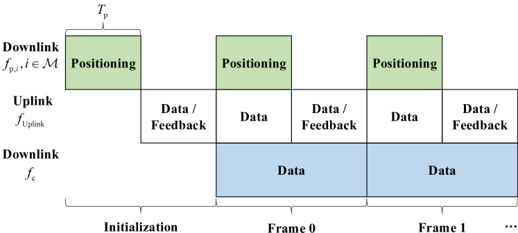
To avoid interference among different functions, the communication frame of the system includes a downlink positioning subframe, a downlink data subframe, and an uplink subframe with different frequencies , and , respectively, as shown in Fig. 1(b). This structure can be implemented by the classical frequency-division multiple access. Besides, the allocated frequencies is an ID of -th LED to distinguish the source of the positioning signals. For the positioning subframe with the duration , LEDs simultaneously transmit positioning signals to the UE, which can estimate the RSS. Although the center controller can use the RSS information to calculate the UE’s location, the issues of the UE privacy and the computing load at the center controller make it reasonable that the UE directly undertakes all the computation tasks. Thus, we assume that the UE is powerful enough to perform the positioning, channel state information (CSI) estimation, and the joint power allocation for the next subframe. In the uplink feedback subframe, the UE only feeds back the CSI and the result of the power allocation to the center controller by infrared communications or RF communications. Finally, the center controller deploys the power allocation results, and selects the LED with the best CSI to transmit data to the UE during the next downlink data subframe. The model can be extended into the multi-UE scenario through a proper multiple-access protocol, which can refer to the classical theory of multi-user networks. For example, based on the TDMA, each UE will be independently served at the allocated slot, which is equivalent to the single-UE case.
II-A Downlink Positioning Subframe
In the positioning subframe, the UE estimates the RSS based on the received signals from LEDs. Specifically, for , the -th LED transmits the positioning symbol , where , , , and . For brevity, we drop the time index throughout the paper, where is denoted by . Hence, the transmitted positioning signal of the -th LED is given as
| (1) |
where indicates the allocated positioning power of the -th LED, and denotes the direct current (DC) bias.
At the UE side, the received light is detected by the PD and usually travels via the line of sight (LOS) and diffuse links, and a DC blocking circuit is adopted to filter the DC component. The received positioning signal from the -th LED can be expressed as
| (2) |
where is the channel gain between the -th LED and the UE, and is the zero-mean Gaussian noise .
Generally, the channel gain can be decomposed as
| (3) |
where and are the channel gains of the LOS and diffuse links between the -th LED and the UE, respectively. For the LOS link, the channel gain is given by[31]
| (4) |
where is the Lambertian index of the LED, denotes the semi-angle, is the effective area of PD, is the electric-optical conversion coefficient, is the optical-electric conversion coefficient, indicates the FoV of PD, denotes the distance from the -th LED to the UE, denotes the angle of irradiance of the -th LED, and denotes the angle of the PD incidence from the -th LED.
On the other hand, the CSI of the diffuse links is always unknown, and the gain of the LOS link is significantly higher than that of the diffuse link [32, 33]. Therefore, to simplify the analysis, we assume that the diffuse links can be ignored, and only the LOS link needs to be considered, i.e., .
Finally, according to the frequency components of the received positioning signal, the UE can detect which LED is in the UE’s FoV and estimate the RSS. Let denote the set of the received LED’s index, and denote the power vector of the received signals from the received LEDs to the UE, where . Without loss of generality, we assume that .
II-B Positioning and Channel Estimation
When at least 3 non-collinear LEDs can be received, using the RSS-based positioning method, the UE’s location estimation can be transformed into a RSS-related estimation problem. For example, utilizing the least squares method[34], the positioning result of the UE can be solved by where denotes the corresponding received power vector at the UE’s Location . Thus, the positioning error is defined as
| (5) |
Generally, the positioning error is assumed to follow two typical probability distribution models: Gaussian distribution and arbitrary distribution.
-
•
Gaussian distribution: If only the mean and variance are known, the Gaussian distribution can maximize the entropy of the uncertain parameter without additive constraints. This model has been adopted in [35, 36, 37] because the CRLB is asymptotically achieved by the maximum-likelihood (ML) estimator even for finite data size[38, 39].
-
•
Arbitrary distribution: The location estimators based on approximate ML[40, 41], and multidimensional scaling (MDS) [42] can also achieve the CRLB. However, the estimation errors do not necessarily follow a Gaussian distribution[43, 35]. In this case, although the distribution of the position error is unavailable, its mean and variance also can be assumed to be known [44, 35, 42].
Based on the RSS and the signal , we can select the -th LED to transmit the downlink data, which is assumed to correspond to the maximum channel gain, i.e.,
| (6) |
and the corresponding LED location is .
If only the LOS link is considered, according to the channel model (4), the estimated CSI between the -th LED and the UE is given by
| (7) |
where .
Due to the positioning error , the channel estimation (7) is imperfect. The corresponding estimated CSI error between the -th LED and the UE is defined as follows
| (8) |
Based on (7) and (8), the channel estimation error is given as
| (9) |
Therefore, is a function of , i.e., .
Based on the result of positioning and channel estimation, the UE can solve the expected power allocation of each LED to optimize the performance of the integrated VLPC system, and the power allocation result can be fed back to the central controller by the uplink. The designed robust power allocation scheme in this paper will be presented in the following section.
II-C Downlink Data Subframe
During the downlink data subframe, the -th LED transmits the data symbol to the UE, where , , and . Then, the transmitted data signal of the -th LED is given by
| (10) |
where indicates the allocated power of the -th LED. In addition, because the -th LED simultaneously transmits the data and positioning signal, the practical transmitted signal can be represented by
| (11) |
Then, the received data signal from the -th LED is given as
| (12) |
where is the received noise, and is independent of .
To ensure that the transmitted signals of VLC are nonnegative, i.e., and , the positioning signal power in (1) and the communication signal power in (10) are, respectively, constrained by
| (13a) | |||
| (13b) | |||
For eye safety and practical illumination requirements, the maximum optical power of VLC signals should also be limited, i.e., , where denotes the maximum optical power of each LED. According to (1) and (10), and are, respectively, limited by
| (14a) | |||
| (14b) | |||
Due to the limited power budget of the practical electrical circuit, the average electrical powers of the signal and signal are also constrained, i.e.,
| (15a) | |||
| (15b) | |||
where denotes the maximum electrical transmitted power.
Meanwhile, considering the limited load capability in practical circuits, the total power of a VLPC integrated system should be constrained, i.e.,
| (17) |
where denotes the maximum total power of the VLPC integrated system.
III Tradeoff Between Positioning and Communication
In this section, we first present the performance metric for positioning and communication, and then we discuss their tradeoff.
III-A CRLB of VLP
In this paper, we adopt the CRLB as the performance metrics for quantifying the localization accuracy of the UE [45, 46, 47]. The CRLB can be achieved by the unbiased estimator since VLC links inherently offer high SNR due to the short transmission distance with the dominant LOS path.
Specifically, we first fix the height of the UE, and focus on the two-dimensional location estimation. Let denote the arbitrary UE location vector, and the vertical height is a known constant perfectly, i.e., . Based on the received signal (2), the log-likelihood function of the received signal is given as
| (18) |
where is a constant and is independent of .
Moreover, let denote the Fisher Information matrix (FIM) of , which is a function of the positioning power . Specifically, the FIM is given as
| (21) |
where
| (22a) | |||
| (22b) | |||
The derivations of (21) are given in Appendix A. Thus, the variance of the zero-mean positioning error is lower bounded by the CRLB [45], i.e.,
| (23) |
III-B Achievable Rates of VLC
Let denote the achievable rate of the UE in the downlink data subframe. Based on the received signal (12), is lower bounded by
| (24a) | ||||
| (24b) | ||||
| (24c) | ||||
where the inequality (24b) holds because of the entropy power inequality (EPI), and (24c) holds since follows the ABG distribution that can achieve the maximum differential entropy [48]. Here, the ABG distribution of signal is given by
| (27) |
where the parameters , , are the solutions of the following equations
| (28a) | |||
| (28b) | |||
| (28c) | |||
where is the error function.
III-C Tradeoff Between Positioning and Communication
The CSI estimation error affects the achievable rate . Furthermore, since and depend on the positioning signal power , the achievable rate not only depends on the communication signal power , but also depends on the positioning signal power . Therefore, there exists an optimal tradeoff between communication power and positioning power for the integrated VLPC system design.
IV Robust Integrated VLPC Design
For any given distribution of the positioning errors, it is hard to design an integrated VLPC scheme for the UE, which always meets the positioning or throughput requirements due to the unbounded errors. However, it is reasonable to make a robust design within the tolerance of uncertainty in practice. In this section, we investigate a chance-constrained robust integrated VLPC design for the two types of positioning error distributions: Gaussian distribution and arbitrary distribution. Specifically, by exploiting the relationship between positioning errors and CSI errors, we focus on designing a VLPC power allocation scheme to minimize the CRLB of VLP under the QoS chance constraint and power constraints.
IV-A VLPC Design With Prefect CSI
Under the minimum rate requirement, the optical and electrical power constraints, the optimal VLPC power allocation to minimize the CRLB of VLP with perfect CSI can be formulated as follows:
| (29a) | ||||
| (29b) | ||||
where denotes the minimum rate requirement. After replacing the constraint (29b) with a more stringent constraint , problem (29) can be rewritten as a convex programming problem, which can be solved by standard optimization solvers such as CVX [49]. In addition, (29) also corresponds to the nonrobust design ignoring the coupling between the positioning error and the estimated CSI error . The optimal communication power and positioning power are denoted by and , respectively.
IV-B Robust VLPC Design with Gaussian Distributed
Considering the relationship between and , we propose the outage chance constraint to handle the minimum rate requirement (29b). When follows the Gaussian distribution, the corresponding chance-constrained VLPC programming problem can be stated as
| (30a) | ||||
| (30b) | ||||
| (30c) | ||||
where denotes the maximum tolerable outage probability.
The robust integrated VLPC design problem (30) is nonconvex and computationally intractable. The main challenge lies in the chance constraint (30b), which does not admit closed-form expressions. In order to handle the chance-constrained problem (30), we first reformulate the chance constraint (30b). Based on the lower bound of the achievable rate (24c), the probability constraint (30b) can be conservatively transformed into the following constraint
| (31) |
Specifically, the constraint can be equivalently reformulated as
| (32) |
where .
Then, by substituting into (32), we have
| (33) |
Moreover, the positioning error can be rewritten as , where . Then, the chance constraint (30b) can be reformulated as
| (34) |
where , , and .
Furthermore, to reformulate the chance constraint (34) into a deterministic form, we invoke the Bernstein-type inequality in Lemma .
Lemma [50] [51]: Let , where is a real symmetric matrix, and . Then, for any , we have
| (35) |
where and is the maximum eigenvalue of matrix .
According to the Bernstein-type inequality, the chance constraint (34) can be conservatively transformed into the following constraint
| (36) |
where . Furthermore, constraint (36) can be equivalently reformulated as
| (37a) | |||
| (37b) | |||
| (37c) | |||
where and are slack variables.
Note that constraint (37a) is convex, but constraints (37b) and (37c) are nonconvex because the matrix inverse is non-convexity-preserving. To tackle this issue, constraints (37b) and (37c) can be transformed to convex forms by exploiting the eigenvalue and singular value properties.
Specifically, the left-hand side of constraint (37b) can be approximated as
| (40) | ||||
| (41) |
where denotes the maximum singular value, and the first inequality is due to , and the second inequality is because the norm is equal to the sum of all singular values. Because the FIM is invertible and semidefinite, we have
| (42a) | ||||
| (42b) | ||||
| (42c) | ||||
where denotes the minimum eigenvalue of the matrix. Thus, an upper bound on the left-hand side of constraint (37b) can be derived, and constraint (37b) can be rewritten with a convex form as follows
| (45) |
Meanwhile, because the positive semidefinite matrix means that its minimum eigenvalue is nonnegative, constraint (37c) can be transformed to a concave form as follows
| (46) |
IV-C Robust VLPC Design with Arbitrary Distributed
In this subsection, we investigate a more practical robust VLPC design scenario, where the central controller has no prior knowledge of the distribution of the position error except for its first and second-order moments, i.e., only the mean and variance of are known. Specifically, although the distribution of is arbitrary, the positioning error variance can achieve the CRLB, i.e., , and the mean of is zero, i.e., .
With the arbitrary distributed , we aim to minimize the CRLB of VLP by optimizing the power allocation subject to the VLC chance constraint and power constraints. Mathematically, the robust VLPC problem can be formulated as follows:
| (48a) | ||||
| (48b) | ||||
Problem (48) appears to be more challenging than problem (30) since less information about the distribution of is known. To reformulate the intractable chance constraints to computationally tractable constraints, (30b) can be equivalently expressed as
| (49) |
Furthermore, the chance constraint (49) can be transformed into a distributionally robust chance constraint, which is given by
| (50) |
where denotes the probability lower bound under the probability distribution and is called the ambiguity set, which includes all the possible position error distributions.
Lemma [52, 53]: Consider a continuous loss function that is concave or quadratic in . The distributionally robust chance constraint is equivalent to the worst-case constraint, which is given by
| (51) |
where is denoted as the CVaR of at the threshold with respect to , defined as
| (52) |
Moreover, is the set of real numbers and , and is an auxiliary variable introduced by the CVaR.
Lemma [52, 53]: Let be a quadratic function of , . The worst-case CVaR can be computed as
| (53a) | ||||
| (53b) | ||||
| (53c) | ||||
where and are the auxiliary variables, and is a matrix defined as
| (54) |
where and are the mean and covariance matrix of random vector , respectively.
The arbitrary distributed positioning error makes the chance constraint lower bound intractable. However, a CVaR-based method can overcome this challenge effectively, which is known as a good convex approximation of the worst-case chance constraint[52, 53]. As is described by Lemmas 2 and 3, for the continuous quadratic function , the distributionally robust chance constraint (50) can be made equivalent to the worst-case CVaR constraint as follows:
| (55a) | |||
| (55b) | |||
| (55c) | |||
where and are two auxiliary variables, and .
The successive convex approximation (SCA) based on the first-order Taylor expansion can be exploited to process the nonconvex constraint (55c). The first-order Taylor expansion of the terms , and is substituted into (55c) to find an affine approximation, which is given by
| (56) |
where , and denote the approximations of , and through
| (57a) | |||
| (57b) | |||
| (57c) | |||
Thus, the chance-constrained problem (48) can be reformulated as follows
| (58) | ||||
For any known and , the joint optimization problem (58) becomes the convex SDP, which can be solved by standard convex programming solvers such as CVX[49]. Toward this end, we transform problem (58) into a series of convex subproblems, which can be solved efficiently through iterations. At the -th iteration, the corresponding convex subproblem is given as
| (59a) | ||||
| (59b) | ||||
Then, the iterations repeat until the termination condition is satisfied, and the optimal solutions and are output. The details of the robust integrated VLPC method for the arbitrary distributed are summarized as Algorithm 1. The proposed SCA algorithm can converge to a stationary point of the original problem after using the CVaR-based method[54]. At each iteration, the subproblem (50) can be efficiently solved with a worst-case complexity , where is the accuracy of the interior-point method[49, 55].
V numerical results
This section presents numerical results to show the proposed robust power allocation schemes for the integrated VLPC system. We consider an indoor VLPC system installed with multiple LEDs on the ceiling, where the room height is , and a corner of a square room denotes the origin of a three-dimensional Cartesian coordinate system . The receiver’s location is , and four numbers of transmitters are considered, namely, 3 LEDs, 4 LEDs, 5 LEDs, and 6 LEDs, where their locations are shown in Fig. 2. According to the channel model (4), it can be verified that all LEDs are within the UE’s FoV. The signal is assumed to be drawn from a uniform distribution , i.e., , . Without loss of generality, we assume that the total power is . According to [27, 28, 45], the other simulation parameters are listed in TABLE III.
| Definition | Value |
|---|---|
| Lambertian index, | |
| Angle of FoV, | |
| Half power angle, | |
| PD effective area, | |
| Conversion coefficient, , | |
| Bandwidth, | |
| DC bias, , | |
| Noise power, , | |
| Maximum optical power, | W |
| Maximum electrical power, | W |
| Positioning subframe length, | s |

V-A Cumulative Distribution Functions of Communication Rates
We first evaluate the robust performance of the proposed power allocation schemes by Monte Carlo simulation, and the cumulative distribution functions (CDF) of the achievable data rate are presented in Fig. 3 and Fig. 4. In the initial stages, there is only a DC signal at each LED to provide illumination and positioning, i.e., , . Then, the random samples of the positioning error are independently generated based on the distribution . The estimated location can be derived by (5). Finally, the result of power allocation is fed into a practical simulation environment to evaluate the achievable data rate . Besides, the mean of is considered as the replacement of the actual location in problems (29), (32), and (48).
Meanwhile, the proposed schemes are also verified by both LOS and diffuse links (LOS+diffuse). According to the classical optical wireless channel model [56], the channel impulse response is given by
| (60) |
where is the power efficiency of the diffuse link, denotes the exponential decay time, is the delay between the LOS signal and the diffuse signal, is the Dirac function, and is the unit step function. We assume that , , and . If the inter-symbol interference (ISI) due to the diffuse link is treated as noise, the achievable rate of the LOS+diffuse link is given by[57, 58]
| (61) |
where and denote the power without ISI and the power with ISI, respectively,
| (62a) | ||||
| (62b) | ||||
| (62c) | ||||
| (62d) | ||||
| (62e) | ||||
| (62f) | ||||
Fig. 3(a) illustrates the CDF of the achievable rate under the assumption of the Gaussian distributed positioning error with LEDs, and different maximum tolerable outage probabilities , and nonrobust () for only the LOS link and the LOS+diffuse link, respectively. For the nonrobust method, the outage probability with only the LOS link is about , and it is close to for the LOS+diffuse case, which significantly exceeds the maximum tolerated outage probability requirement. On the other hand, the outage probability of the proposed robust power allocation in Section IV-B is close to , even for the LOS+diffuse case, which is well below the requirements and . Fig. 3(b) depicts the same results for LEDs. For the same and channel type, the CDF curves in Fig. 3(b) are lower than those in Fig. 3(a). In other words, the conservatism of the proposed robust scheme can be reduced slightly as the number of LEDs increases. In addition, if the other settings are the same, the achievable rate with is highest, and the rate of the nonrobust case is lowest. Thus, it leads to a higher actual rate to guarantee stricter outage probability constraint.
Fig. 4 shows the case of the arbitrary positioning error distribution, and the chance constraint of the achievable rate is also satisfied. Comparing with Fig. 3, the CVaR-based scheme provides a higher communication rate than the Bernstein-based scheme for the same scenario. Thus, the CVaR-based scheme is more robust than the scheme based on the Bernstein-type inequality, because of less utilized prior information. On the other hand, the CVaR-based scheme can be applied widely in practical scenarios.

(a)

(b)

(a)

(b)
V-B CRLB Versus the Rate Threshold
In this subsection, we show the relationship between the positioning error and the communication requirement for the nonrobust and two proposed robust schemes. The square root of the CRLB versus the achievable rate threshold is investigated in Fig. 5(a) and Fig. 5(b) under the Gaussian and arbitrary positioning error distributed assumptions, respectively. To represent the average performance, it is assumed that there is only the LOS channel, and the UE’s location estimation is the actual position, i.e., .

(a)

(b)
Fig. 5(a) shows the results under the Gaussian distributed assumption with LEDs, and the maximum tolerable outage probabilities are , and nonrobust case. Since , the nonrobust case is equivalent to the perfect positioning case. We observe that the positioning performance degrades as the minimum rate requirement increases, which means that there is a tradeoff between the communication performance and the positioning precision. When the LED number is fixed, and the rate threshold is low enough, such as , the CRLB changes slowly. However, if is high enough, it degrades rapidly. Besides, for the same rate threshold and the LED number, stricter will lead to worse CRLB. On the other hand, the CRLB can be obviously reduced as the LED number increases from to .
Comparing with Fig. 5(a), Fig. 5(b) is set to the same scenario except for the distribution assumption, and there are similar trends of the CRLB versus the rate for different parameters. However, the CVaR-based scheme leads to more drastic positioning performance loss versus the rate threshold and the outage probabilities threshold .
V-C Power Allocation Versus the Rate Threshold
To further derive the performance tradeoff between communication and positioning, the power allocation results versus the rate threshold are illustrated in Fig. 6 and Fig. 7, assuming Gaussian and arbitrary distributed positioning error, respectively. Other design parameters are the same as those in Section V-B.

(a)

(b)

(a)

(b)
From Fig. 6 and Fig. 7, the allocated communication power increases as the minimum rate requirement increases, and the rate of change also increases continuously. To minimize the CRLB, the remaining power is always allocated to the positioning signals as much as possible within the constraints. For problems (29), (30), and (48), the allocated positioning power should satisfy . Due to the limited total power, will decrease as the minimum rate requirement increases, which leads to the CRLB degradation.
In addition, more power will be allocated to VLC, if a stricter outage probability constraint or a more robust power allocation scheme is adopted. This causes the sort of achievable rates in Fig. 3 and Fig. 4. When other settings are the same, the achievable rate with is the highest, and the rate of the nonrobust case is the lowest. Meanwhile, the CVaR-based scheme provides a higher communication rate than the Bernstein-based scheme for the same scenario. This is also the reason for the variation of the CRLB, as shown in Fig. 5 with different parameters and schemes.
According to (9), (30c) and (48b), the positioning error distribution can directly influence the distribution of the channel estimation error. Although the allocated positioning power with LEDs approximates the power with LEDs in both Fig. 6 and Fig. 7, the more LEDs can improve the positioning performance, as illustrated in Fig. 5. Thus, it can reduce the variance of the channel estimation error to increase the LED number. For communication, the conservatism of the robust schemes can be mitigated, as shown in Fig. 3 and Fig. 4.
V-D Cumulative Distribution Functions of Positioning Errors
To evaluate the positioning performance loss of robust VLPC schemes, the RSS-based triangulation process was simulated with only the LOS link and the LOS+diffuse link. The location is estimated using the nonlinear least squares method. Besides, the positioning error is calculated using the root-square error (RSE). The CDFs of positioning errors are shown in Fig. 8.
From both Fig. 8(a) and Fig. 8(b), two robust VLPC power allocation schemes lead to only a slight loss of positioning precision. Thus, the proposed robust power allocation schemes are also effective for VLP.

(a)

(b)
VI conclusion
In this work, we investigated the inherent coupling between VLP and VLC through the relationship between the optical channel and the location. In other words, channel estimation can be implemented using the positioning result. After deriving the CRLB for VLP and the achievable rate for VLC, we unveiled the tradeoff between VLP and VLC by the relationship between the channel estimation error and the positioning error. Furthermore, we proposed two robust power allocation schemes for VLPC to minimize the CRLB under the power constraints and QoS requirements, where the positioning error distributions are assumed to follow either the Gaussian distribution or an arbitrary distribution with a known mean and variance. Under the Gaussian distributed assumption, the Bernstein-type inequality is utilized to tackle the communication rate outage constraints, and the problem was converted into a stricter convex SDP by exploiting the matrix norm. For the arbitrary distributed case, the problem was approximated by a more tractable form through the worst-case CVaR and SCA based on the first-order Taylor expansion. Finally, our simulation results demonstrated the effectiveness of our two proposed robust VLPC power allocation schemes for both localization and communications.
Appendix A Derivation of the formulation (21)
The derivative of the log-likelihood function with respect to is given by[38]
| (63) | ||||
| (64) |
where and can be expressed as
| (65) | |||
| (66) |
Furthermore, the FIM can be denoted as an explicit function between the position power and the unknown UE location in the 2D plane.
| (69) |
where the elements of (69) are given as
| (70) | ||||
| (71) | ||||
| (72) | ||||
| (73) |
References
- [1] “Cisco service provider Wi-Fi: A platform for business innovation and revenue generation,” http://www.cisco.com/c/en/us/solutions/collateral/service-provider/serviceprovider-wi-fi/solutionoverviewc22-642482.html.
- [2] P. S. Farahsari, A. Farahzadi, J. Rezazadeh, and A. Bagheri, “A Survey on Indoor Positioning Systems for IoT-Based Applications,” IEEE Internet Things J., vol. 9, no. 10, pp. 7680–7699, May 2022.
- [3] F. Alam, N. Faulkner, and B. Parr, “Device-Free Localization: A Review of Non-RF Techniques for Unobtrusive Indoor Positioning,” IEEE Internet Things J., vol. 8, no. 6, pp. 4228–4249, Mar. 2021.
- [4] T. Kamalakis, Z. Ghassemlooy, S. Zvanovec, and L. Nero Alves, “Analysis and simulation of a hybrid visible-light/infrared optical wireless network for IoT applications,” J. Opt. Commun. Netw., vol. 14, no. 3, pp. 69–78, Mar. 2022.
- [5] A. Memedi and F. Dressler, “Vehicular Visible Light Communications: A Survey,” IEEE Commun. Surv. Tutor., vol. 23, no. 1, pp. 161–181, Firstquarter 2021.
- [6] L. E. M. Matheus, A. B. Vieira, L. F. M. Vieira, M. A. M. Vieira, and O. Gnawali, “Visible Light Communication: Concepts, Applications and Challenges,” IEEE Commun. Surv. Tutor., vol. 21, no. 4, pp. 3204–3237, Fourthquarter 2019.
- [7] J. Luo, L. Fan, and H. Li, “Indoor positioning systems based on visible light communication: State of the art,” IEEE Commun. Surv. Tutor., vol. 19, no. 4, pp. 2871–2893, Aug. 2017.
- [8] M. F. Keskin, A. D. Sezer, and S. Gezici, “Localization via visible light systems,” Proc. IEEE, vol. 106, no. 6, pp. 1063–1088, Jun. 2018.
- [9] X. Zhang, J. Duan, Y. Fu, and A. Shi, “Theoretical accuracy analysis of indoor visible light communication positioning system based on received signal strength indicator,” J. Lightw. Technol., vol. 32, no. 21, pp. 4180–4186, Nov 2014.
- [10] F. Alam, N. Faulkner, M. Legg, and S. Demidenko, “Indoor visible light positioning using spring-relaxation technique in real-world setting,” IEEE Access, vol. 7, pp. 91347–91359, Jul. 2019.
- [11] P. Du, S. Zhang, C. Chen, H. Yang, W. Zhong, R. Zhang, A. Alphones, and Y. Yang, “Experimental demonstration of 3D visible light positioning using received signal strength with low-complexity trilateration assisted by deep learning technique,” IEEE Access, vol. 7, pp. 93986–93997, Jul. 2019.
- [12] X. Sun, Y. Zhuang, J. Huai, L. Hua, D. Chen, Y. Li, Y. Cao, and R. Chen, “RSS-Based Visible Light Positioning Using Nonlinear Optimization,” IEEE Internet Things J., vol. 9, no. 15, pp. 14137–14150, Aug. 2022.
- [13] A. Şahin, Y. S. Eroğlu, İ. Gğvenç, N. Pala, and M. Yüksel, “Hybrid 3-D localization for visible light communication systems,” J. Lightw. Technol., vol. 33, no. 22, pp. 4589–4599, Nov. 2015.
- [14] X. Sun, J. Duan, Y. Zou, and A. Shi, “Impact of multipath effects on theoretical accuracy of TOA-based indoor VLC positioning system,” Photon. Res., vol. 3, no. 6, pp. 296–299, Dec 2015.
- [15] W. Gu, M. Aminikashani, P. Deng, and M. Kavehrad, “Impact of multipath reflections on the performance of indoor visible light positioning systems,” J, Lightw. Technol., vol. 34, no. 10, pp. 2578–2587, May 2016.
- [16] P. Du, S. Zhang, C. Chen, A. Alphones, and W. Zhong, “Demonstration of a low-complexity indoor visible light positioning system using an enhanced TDOA scheme,” IEEE Photon. J., vol. 10, no. 4, pp. 1–10, May 2018.
- [17] M. F. Keskin, S. Gezici, and O. Arikan, “Direct and two-step positioning in visible light systems,” IEEE Trans. Commun., vol. 66, no. 1, pp. 239–254, Jan. 2018.
- [18] X. Lin and L. Zhang, “Intelligent and practical deep learning aided positioning design for visible light communication receivers,” IEEE Commun. Lett., vol. 24, no. 3, pp. 577–580, Mar. 2020.
- [19] B. Lin, X. Tang, Z. Ghassemlooy, C. Lin, and Y. Li, “Experimental demonstration of an indoor VLC positioning system based on OFDMA,” IEEE Photon. J., vol. 9, no. 2, pp. 1–9, Apr. 2017.
- [20] D. Chen, K. Fan, J. Wang, H. Lu, J. Jin, L. Feng, H. Chen, Z. Xue, and Y. Wang, “Integrated visible light communication and positioning CDMA system employing modified ZCZ and Walsh code,” Opt. Express, vol. 30, no. 22, pp. 40455–40469, Oct 2022.
- [21] L. Shi, B. Béchadergue, L. Chassagne, and H. Guan, “Joint visible light sensing and communication using -CAP modulation,” IEEE Trans. Broadcast., vol. 69, no. 1, pp. 276–288, 2023.
- [22] S. Shao, A. Salustri, A. Khreishah, C. Xu, and S. Ma, “R-VLCP: Channel modeling and simulation in retroreflective visible light communication and positioning systems,” IEEE Internet of Things J., pp. 1–1, 2023 (Early Access).
- [23] J. Jin, H. Lu, J. Wang, J. Huang, L. Feng, D. Chen, H. Chen, T. Dong, Y. Su, and Y. Wang, “Adaptive feedback threshold based demodulation for mobile visible light communication and positioning integrated system,” Opt. Express, vol. 30, no. 8, pp. 13331–13344, Apr 2022.
- [24] H. Yang, P. Du, W. Zhong, C. Chen, A. Alphones, and S. Zhang, “Reinforcement learning-based intelligent resource allocation for integrated VLCP systems,” IEEE Wireless Commun. Lett., vol. 8, no. 4, pp. 1204–1207, Aug. 2019.
- [25] Y. Xu, Z. Wang, P. Liu, J. Chen, S. Han, C. Yu, and J. Yu, “Accuracy analysis and improvement of visible light positioning based on VLC system using orthogonal frequency division multiple access,” Opt. Express, vol. 25, no. 26, pp. 32618–32630, Dec. 2017.
- [26] H. Yang, C. Chen, W.-D. Zhong, A. Alphones, S. Zhang, and P. Du, “Demonstration of a quasi-gapless integrated visible light communication and positioning system,” IEEE Photon. Technol. Lett., vol. 30, no. 23, pp. 2001–2004, Dec. 2018.
- [27] H. Yang, W.-D. Zhong, C. Chen, A. Alphones, P. Du, S. Zhang, and X. Xie, “Coordinated resource allocation-based integrated visible light communication and positioning systems for indoor IoT,” IEEE Trans. Wireless Commun., vol. 19, no. 7, pp. 4671–4684, Jul. 2020.
- [28] H. Yang, W.-D. Zhong, C. Chen, A. Alphones, and P. Du, “QoS-driven optimized design-based integrated visible light communication and positioning for indoor IoT networks,” IEEE Internet Things J., vol. 7, no. 1, pp. 269–283, Jan. 2020.
- [29] R. K. Pal, S. P. Dash, S. Joshi, and D. Ghose, “Channel estimation and performance analysis of a wide-FOV visible light communication system with random receiver orientation and location,” IEEE Trans. Wireless Commun., vol. 22, no. 3, pp. 1964–1979, 2023.
- [30] S. Ma, R. Yang, B. Li, Y. Chen, H. Li, Y. Wu, M. Safari, S. Li, and N. Al-Dhahir, “Optimal power allocation for integrated visible light positioning and communication system with a single LED-lamp,” IEEE Trans. Commun., vol. 70, no. 10, pp. 6734–6747, 2022.
- [31] J. M. Kahn and J. R. Barry, “Wireless infrared communications,” Proc. IEEE, vol. 85, no. 2, pp. 265–298, Feb 1997.
- [32] T. Fath and H. Haas, “Performance comparison of MIMO techniques for optical wireless communications in indoor environments,” IEEE Trans. Commun., vol. 61, no. 2, pp. 733–742, Feb. 2013.
- [33] T. Q. Wang, Y. A. Sekercioglu, and J. Armstrong, “Analysis of an optical wireless receiver using a hemispherical lens with application in MIMO visible light communications,” J. Lightwave Technol., vol. 31, no. 11, pp. 1744–1754, Apr. 2013.
- [34] K. Cengiz, “Comprehensive Analysis on Least-Squares Lateration for Indoor Positioning Systems,” IEEE Internet Things J., vol. 8, no. 4, pp. 2842–2856, Feb. 2021.
- [35] T. Wang, G. Leus, and L. Huang, “Ranging energy optimization for robust sensor positioning based on semidefinite programming,” IEEE Trans. on Sig. Process., vol. 57, no. 12, pp. 4777–4787, Jul. 2009.
- [36] V. Lottici, A. DÁndrea, and U. Mengali, “Channel estimation for ultra-wideband communications,” IEEE J. Sel. Areas Commun., vol. 20, no. 9, pp. 1638–1645, Dec. 2002.
- [37] S. Gezici, Z. Tian, and G. B. Giannakis, “Localization via ultrawideband radios,” IEEE Sig. Process. Mag., vol. 22, no. 4, pp. 70–84, Jul. 2005.
- [38] S. M. Kay, Fundamentals of Statistical Signal Processing-Estimation Theory, Englewood Cliffs, NJ: Prentice-Hall, 1993.
- [39] K. W. Cheung, H. C. So, W. . Ma, and Y. T. Chan, “Least squares algorithms for time-of-arrival-based mobile location,” IEEE Trans. on Sig. Process, vol. 52, no. 4, pp. 1121–1130, Apr. 2004.
- [40] Y. Chan, H. Y. C. Hang, and P. Ching, “Exact and approximate maximum likelihood localization algorithms,” IEEE Trans. Veh. Technol., vol. 55, no. 1, pp. 10–16, Jan. 2006.
- [41] K. W. Cheung, W. K. Ma, and H. C. So, “Accurate approximation algorithm for TOA-based maximum likelihood mobile location using semidefinite programming,” in 2004 IEEE International Conference on Acoustics, Speech, and Signal Processing, vol. 2, pp. ii–145, May 2004.
- [42] H. Wei, Q. Wan, Z. Chen, and S. Ye, “A novel weighted multidimensional scaling analysis for time-of-arrival-based mobile location,” IEEE Trans. Signal Process., vol. 56, no. 7, pp. 3018–3022, Jul. 2008.
- [43] F. Gustafsson and F. Gunnarsson, “Mobile positioning using wireless networks: possibilities and fundamental limitations based on available wireless network measurements,” IEEE Signal Process. Mag., vol. 22, no. 4, pp. 41–53, Jul. 2005.
- [44] D. J. Torrieri, “Statistical theory of passive location systems,” IEEE Trans. Aerosp. Electron. Syst., vol. AES-20, no. 2, pp. 183–198, Mar. 1984.
- [45] M. F. Keskin, A. D. Sezer, and S. Gezici, “Optimal and robust power allocation for visible light positioning systems under illumination constraints,” IEEE Trans. Commun., vol. 67, no. 1, pp. 527–542, Jan. 2019.
- [46] H. L. V., Trees, Detection, Estimation, and Modulation Theory, NY,USA:Wiley, 2004.
- [47] H. V. Poor, An Introdunction to Signal Detection and Estimation, NY, USA: Springer-Verlag, 1994.
- [48] S. Ma, R. Yang, H. Li, Z.-L. Dong, H. Gu, and S. Li, “Achievable rate with closed-form for SISO channel and broadcast channel in visible light communication networks,” J. Lightw. Technol., vol. 35, no. 14, pp. 2778–2787, Jul. 2017.
- [49] M. Grant and S. Boyd, “CVX: Matlab software for disciplined convex programming, version 2.1,” http://cvxr.com/cvx, Mar. 2014.
- [50] K. Wang, A. M. So, T. Chang, W. Ma, and C. Chi, “Outage constrained robust transmit optimization for multiuser MISO downlinks: Tractable approximations by conic optimization,” IEEE Trans. Signal Process., vol. 62, no. 21, pp. 5690–5705, Nov. 2014.
- [51] S. Ma, Y. He, J. Dai, M. Zhang, H. Li, and S. Li, “Robust beamforming for downlink non-orthogonal multiple access network,” in 2017 IEEE/CIC ICCC, pp. 1–6, Oct. 2017.
- [52] S. Zymler, D. Kuhn, and B. Rustem, “Distributionally robust joint chance constraints with second-order moment information,” Math. Program., vol. 137, no. 1, pp. 167–198, Feb. 2013.
- [53] Y. Zhang, B. Li, F. Gao, and Z. Han, “A robust design for ultra reliable ambient backscatter communication systems,” IEEE Internet Things J., vol. 6, no. 5, pp. 8989–8999, Oct. 2019.
- [54] R. Zhou and D. P. Palomar, “Solving High-Order Portfolios via Successive Convex Approximation Algorithms,” IEEE Trans. Signal Process., vol. 69, pp. 892–904, 2021.
- [55] Z.-q. Luo, W.-k. Ma, A. So, Y. Ye, and S. Zhang, “Semidefinite Relaxation of Quadratic Optimization Problems,” IEEE Signal Process. Mag., vol. 27, no. 3, pp. 20–34, May 2010.
- [56] V. Jungnickel, V. Pohl, S. Nonnig, and C. von Helmolt, “A physical model of the wireless infrared communication channel,” IEEE J. Sel. Areas Commun., vol. 20, no. 3, pp. 631–640.
- [57] J. Chen and T. Shu, “Impact of multiple reflections on secrecy capacity of indoor VLC system,” in Information and Communications Security, J. Zhou, X. Luo, Q. Shen, and Z. Xu, Eds., Cham, pp. 105–123, Springer International Publishing, 2020.
- [58] S. Ma, H. Li, Y. He, R. Yang, S. Lu, W. Cao, and S. Li, “Capacity Bounds and Interference Management for Interference Channel in Visible Light Communication Networks,” IEEE Trans. Wirel. Commun., vol. 18, no. 1, pp. 182–193.