Robust minimum divergence estimation
in a spatial Poisson point process

Species distribution modeling (SDM) is critical to evaluate biodiversity, conservation and management planning, impacts on human activities, and so on (Fithian and Hastie, 2013; Schmeller et al., 2018). The presence-absence (PA) data for a species of interest require dedicated surveys per spatial unit; thus, such data are difficult and expensive to obtain. In some cases, the only available data are from museum or herbarium records of locations where the species were observed. In recent years, the development of geographic information systems has enabled ecologists to obtain knowledge of the environment of the study area without conducting field surveys. As a result, presence-only (PO) data have become readily available and research based on the PO data has become more active. However, the PO data often consist of observational surveys rather than the designed surveys, and thus require special attention in the data analysis.

Several statistical and machine learning approaches have been developed to estimate the relative probability or intensity that reflects habitat suitability or abundance of the species of interest. Some methods are based on the joint likelihood of the presence and environmental variables, or on the partial likelihood (Lancaster and Imbens, 1996; Lele and Keim, 2006; Lele, 2009). The application of the spatial Poisson point process (PPP) model to the PO data has been proposed (Warton and Shepherd, 2010; Chakraborty et al., 2011); this model is closely related to the maximum entropy (Maxent) model familiar to ecologists (Fithian and Hastie, 2013; Renner and Warton, 2013). These models can be considered essentially the same method in the sense that they are based on equivalent likelihoods and estimate the equivalent relative probability (or intensity) of presence (Wang and Stone, 2019).

The present paper focuses on the spatial PPP model. In the data analysis of the PO data, it is necessary to be aware of bias due to some reasons. Various methods have been discussed to deal with the sampling bias because the PO data usually suffer from the sampling bias due to heterogeneity in sampling efforts. These methods involve identifying and estimating the effect of bias on presence and then thinning or eliminating it (Dudík et al., 2005; Fithian et al., 2015; Komori et al., 2020). On the other hand, heterogeneous observations of presence occur due to several reasons, such as incorrect or missing geo-coordinates, taxonomic misidentification, and taxonomic shifts in the PO data (Thessen and Patterson, 2011; Wiser, 2016; Serra-Diaz et al., 2017). In fact, Serra-Diaz et al. (2017) noted that a median of 10$\%$ (up to 30$\%$) of presence locations per species across 60,065 tree species were either in highly urbanized areas or outside typical habitat areas, which can have a significant effect in assessing habitat suitability. The heterogeneous observation can have a negative impact on the predictive performance of SDM, e.g., area under the operating characteristic curve (AUC), sensitivity, specificity, and true skill statistic (Liu et al., 2018). Filtering the dataset improves the performance of SDM; however, the contaminated data cannot be automatically corrected because the specialized knowledge and the time-consuming manual checking are required (Belbin et al., 2013; Mesibov, 2013; Velásquez-Tibatá et al., 2019). For large datasets, manually checking the species information introduces exorbitant costs.

Maximum likelihood estimation is usually employed for the PPP model, although it is known that the maximum likelihood estimation is not robust against heterogeneous observations. Despite the PO data are frequently contaminated by heterogeneous observations, to the best of our knowledge, statistical methods for dealing with this issue are rarely discussed, e.g., an M-estimation (Assunção and Guttorp, 1999), and a residual analysis for spatial point process (Baddeley et al., 2005). Robust methods for parameter estimation have been developed on the basis of information divergences to which the Kullback-Leibler (KL) divergence extends (see, e.g., Basu et al., 1998; Fujisawa and Eguchi, 2008; Eguchi and Komori, 2022). The present paper proposes a robust parameter estimation based on the Bregman divergence of intensity functions for the thinned PPP models. The proposed method is characterized by weighting the log-likelihood equation by an influence of heterogeneous observation.

The rest of this paper is organized as follows. Section 2 introduces the spatial PPP model. Section 3 provides a robust parameter estimation method for the thinned PPP model and discusses the robustness to the heterogeneous observation. Section 4 conducts some simulation studies to evaluate the performance of the proposed method. Section 5 presents the analysis of the vascular plant data in Japan. Finally, Section 6 discusses the findings.

Consider a PPP that occurs in the two-dimensional Euclidean space $\mathbb{R}^{2}$. For a study area $\mathscr{A}\subset\mathbb{R}^{2}$, let $\lambda(s)$ denote an intensity function for any site $s\in\mathscr{A}$ and let $\{s_{1},\dots,s_{m}\}$ denote $m$ presence locations in $\mathscr{A}$. Assume that (i) the total number $m$ is a sample from a Poisson distribution with intensity $\int_{\mathscr{A}}\lambda(s)ds$ and that (ii) the presence locations $(s_{i})$ are independent and identically distributed samples of a random variable with the probability function $\lambda(s)/\int_{\mathscr{A}}\lambda(s)ds$ for $s\in\mathscr{A}$. The intensity function can be modeled in a complicated form. For simplicity, this paper assumes a log-linear model for the intensity function; that is, $\log\lambda_{\mbox{\tiny\boldmath$\beta$}}(s)=\mbox{\boldmath$\beta$}^{\top}\mbox{\boldmath$x$}(s)$, where $\mbox{\boldmath$\beta$}=(\beta_{0},\beta_{1},\dots,\beta_{p})^{\top}$ is a coefficient parameter vector, and $\mbox{\boldmath$x$}(s)=(1,x_{1}(s),\dots,x_{p}(s))^{\top}$ is an environmental variable vector at a location $s$. To deal with the bias due to the heterogeneity of sampling effort, the thinned PPP was developed (Dudík et al., 2005; Fithian et al., 2015). Consider the modeling of a PPP by the thinning PPP with the intensity $\lambda_{\mbox{\tiny\boldmath$\theta$}}(s)=\lambda_{\mbox{\tiny\boldmath$\beta$}}(s)b_{\mbox{\tiny\boldmath$\alpha$}}(s)$ using a detection probability $b_{\mbox{\tiny\boldmath$\alpha$}}(s)$ for a site $s\in\mathscr{A}$, where $\mbox{\boldmath$\alpha$}=(\alpha_{1},\dots,\alpha_{q})^{\top}$ is a parameter vector and $\mbox{\boldmath$\theta$}=(\mbox{\boldmath$\beta$}^{\top},\mbox{\boldmath$\alpha$}^{\top})^{\top}$. This paper assumes a logistic-linear model for the detection probability; that is, $\mathop{\rm logit}b_{\mbox{\tiny\boldmath$\alpha$}}(s)=\mbox{\boldmath$\alpha$}^{\top}\mbox{\boldmath$z$}(s)$, where $\mbox{\boldmath$z$}(s)=(z_{1}(s),\dots,z_{q}(s))^{\top}$ is a vector of sampling-bias variable, e.g., distance from a road or an urbanized area.

The log-likelihood function of the thinned PPP model is defined by

$\displaystyle l(\mbox{\boldmath$\theta$})=\sum_{i=1}^{m}\log\left\{\lambda_{\mbox{\tiny\boldmath$\theta$}}(s_{i})\right\}-\int_{\mathscr{A}}\lambda_{\mbox{\tiny\boldmath$\theta$}}(s)ds.$

(1)

Noting that the integral over a study area in equation (1) cannot be exactly calculated, a numerical approximation method has been proposed to estimate the integral using quadrature weights (Berman and Turner, 1992). Without loss of generality, we set up a location vector $\{s_{1},\dots,s_{r}\}$ when the study area $\mathscr{A}$ is split into $n$ grid cells, where $r=n+m-m^{(n)}$, $m^{(n)}$ is the number of grid cells that contain at least one presence location, and $\{s_{m+1},\dots,s_{r}\}$ are the centers of the grid cells that contain no presence location. The approximated log-likelihood function is then given by

$\displaystyle l(\mbox{\boldmath$\theta$})=\sum_{i=1}^{r}\left[d_{i}\log\left\{\lambda_{\mbox{\tiny\boldmath$\theta$}}(s_{i})\right\}-w_{i}\lambda_{\mbox{\tiny\boldmath$\theta$}}(s_{i})\right],$

(2)

where $d_{i}=I(i\in\{1,\dots,m\})$, $I(\cdot)$ is the indicator function, and $w_{i}$ is a quadrature weight for a location $s_{i}$. We regard the area of a grid cell divided by the number of locations $\{s_{1},\dots,s_{r}\}$ contained in the cell as the quadrature weight $w_{i}$ in the same manner as Renner and Warton (2013). That is, $w_{i}=|\mathscr{A}|/(nm_{i}^{+})$, where $|\mathscr{A}|$ is the area of $\mathscr{A}$, $m_{i}^{+}=\max\{1,m_{i}\}$, and $m_{i}$ is the number of presence locations at a grid cell $s_{i}$. The likelihood equations can be obtained by

	$\displaystyle\frac{\partial}{\partial\mbox{\boldmath$\beta$}}l(\mbox{\boldmath$\theta$})$	$\displaystyle=\sum_{i=1}^{r}\varepsilon_{\mbox{\tiny\boldmath$\beta$}}(\mbox{\boldmath$\theta$},s_{i})=\sum_{i=1}^{r}\{d_{i}-w_{i}\lambda_{\mbox{\tiny\boldmath$\theta$}}(s_{i})\}\mbox{\boldmath$x$}(s_{i})=\mbox{\boldmath$0$}_{1+p},$		(3)
	$\displaystyle\frac{\partial}{\partial\mbox{\boldmath$\alpha$}}l(\mbox{\boldmath$\theta$})$	$\displaystyle=\sum_{i=1}^{r}\varepsilon_{\mbox{\tiny\boldmath$\alpha$}}(\mbox{\boldmath$\theta$},s_{i})=\sum_{i=1}^{r}\frac{1}{1+\exp\left(\mbox{\boldmath$\alpha$}^{\top}\mbox{\boldmath$z$}(s_{i})\right)}\{d_{i}-w_{i}\lambda_{\mbox{\tiny\boldmath$\theta$}}(s_{i})\}\mbox{\boldmath$z$}(s_{i})=\mbox{\boldmath$0$}_{q},$		(4)

where $\mbox{\boldmath$0$}_{k}$ indicates a $k$-dimensional zero vector. Solving the likelihood equations, the maximum likelihood estimator (MLE) of parameter $\theta$ is obtained. The intensity function is estimated by plugging the MLEs into the intensity model, $\lambda_{\mbox{\tiny\boldmath$\beta$}}(s)=\exp\{\mbox{\boldmath$\beta$}^{\top}\mbox{\boldmath$x$}(s)\}$, and setting $\mbox{\boldmath$\alpha$}=\mbox{\boldmath$0$}$ that means the sampling-bias effect is removed.

If the species distribution model is correctly specified, then the maximum likelihood method would yield accurate conclusions, even in the presence of sampling bias. However, we must be cautious in situations where model misspecification occurs in practical ecological studies. A non-negligible degree of misspecification can render the MLE unreliable and lead to incorrect inference. For instance, unobservable feature variables might cause the underlying intensity function to deviate slightly from parametric intensity functions, such as interactions with other species. The following section will address this issue and propose a new estimation method.

We are concerned with various possibilities for the misspecification of the thinned PPP model with the parametric intensity function $\lambda_{\mbox{\tiny\boldmath$\theta$}}(s)$ as introduced in section 2. Our main objective is to propose a robust estimation method for the parameter $\theta$. To achieve this, we employ a weighted likelihood equation approach. We focus on the values of parametric intensities $\{\lambda_{\mbox{\tiny\boldmath$\theta$}}(s_{i}):i=1,..,r\}$, which should represent the species abundance. Suppose that occurrences are partially generated by a heterogeneous point process different from the assumed model with the parameter $\theta$. In this case, the values of parametric intensities corresponding to heterogeneous processes have a small magnitude. In light of this, we propose a weighted likelihood equation for $\mbox{\boldmath$\theta$}=(\mbox{\boldmath$\beta$}^{\top},\mbox{\boldmath$\alpha$}^{\top})^{\top}$ as follows:

	$\displaystyle\sum_{i=1}^{r}F(\tau\lambda_{\mbox{\tiny\boldmath$\theta$}}(s_{i}))\varepsilon_{\mbox{\tiny\boldmath$\beta$}}(\mbox{\boldmath$\theta$},s_{i})$	$\displaystyle=\mbox{\boldmath$0$}_{1+p},$		(5)
	$\displaystyle\sum_{i=1}^{r}F(\tau\lambda_{\mbox{\tiny\boldmath$\theta$}}(s_{i}))\varepsilon_{\mbox{\tiny\boldmath$\alpha$}}(\mbox{\boldmath$\theta$},s_{i})$	$\displaystyle=\mbox{\boldmath$0$}_{q},$		(6)

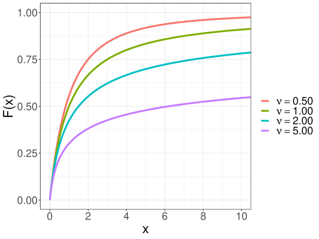
where $\tau>0$ is a constant tuning parameter and $F(\cdot)$ is a cumulative distribution function for the value of the intensity function. We refer to the estimator of $\beta$ of interest, say $\hat{\mbox{\boldmath$\beta$}}_{\tau}$, based on equations (5) and (6) as the minimum intensity divergence estimator (MIDE). Here we adopt the Pareto type II distribution

$\displaystyle F(x)=1-\big{(}1+{\nu}x\big{)}^{-\frac{1}{\nu}}$

(7)

for $x>0$, where $\nu>0$ is a shape parameter. See Figure 1. This distribution has a long tail, which achieves stable estimation by preventing extremely large weights. For practical purposes, we will fix $\nu=1$. The weight function $F(\tau\lambda(s_{i},\theta))$ expresses the magnitude of the intensity function at point $s_{i}$, and calibrates the model correctness by suppressing the influence of heterogeneous observations in the weighted likelihood function. We derive the estimating equations (5) and (6) in terms of minimization of a specific example of Bregman divergence from the true intensity function to the parametric intensity function $\lambda_{\mbox{\tiny\boldmath$\theta$}}(s)$. A detailed derivation of equations (5) and (6) are provided in Appendix A. The property of the divergence automatically leads to the consistency of the proposed estimator for $\theta$. The consistency and asymptotic normality of the MIDE can be derived (see Appendix B for the details). When the tuning parameter $\tau$ goes to $\infty$, then the MIDE reduces to the MLE from equations (3) and (4) because all the weights of the estimating equations are equal to 1. Therefore, the MLE has no chance of suppressing the influence of heterogeneous observations.

To simultaneously carry out the shrinkage estimation and the variable selection, we consider the penalized loss function with an $L_{1}$ penalty (Tibshirani, 1996) as follows.

$\displaystyle l^{\phi}_{\Xi}(\mbox{\boldmath$\beta$},\mbox{\boldmath$\alpha$})=l_{\Xi}(\mbox{\boldmath$\beta$},\mbox{\boldmath$\alpha$})+\sum_{k=0}^{p}\phi_{k}|\beta_{k}|,$

(8)

where $l_{\Xi}$ is the loss function minimized by solving the estimating equations (5) and (6) and is given by equation (13) in Appendix A, $\phi_{0}=0$, and $\phi_{k}=\phi$ ($k\neq 0$, $\phi\geq 0$) is a constant tuning parameter. The loss function has no penalties for the intercept parameter $\beta_{0}$ of the intensity function and the coefficient paramter $\alpha$ for the detection probability model. The gradient ascent method (Goeman, 2010) can be used to compute the $L_{1}$ penalized estimates. The detailed computation algorithm is provided in Appendix C.

The root trimmed mean squared prediction error (RTMSPE) is employed to select the appropriate values of the tuning parameters $\tau$ and $\phi$ by removing heterogeneous observations. The RTMSPE is given by

$\displaystyle{\rm RTMSPE}_{\delta}=\sqrt{\frac{1}{h_{\delta}}\sum_{i=1}^{h_{\delta}}e^{2}_{[i]}}\qquad(0<\delta<1),$

(9)

where $h_{\delta}=\lfloor(n+1)\delta\rfloor$ and $e^{2}_{[1]}\leq\cdots\leq e^{2}_{[n]}$ are the order statistics of $[m_{[1]}-\lambda_{\hat{\mbox{\tiny\boldmath$\theta$}}}(s_{[1]})]^{2},\dots,[m_{[n]}-\lambda_{\hat{\mbox{\tiny\boldmath$\theta$}}}(s_{[n]})]^{2}$ for grid cells ($s_{[1]},\dots,s_{[n]}$) that do not overlap each other and the number of observations ($m_{[1]},\dots,m_{[n]}$) in the cells with a estimate $\hat{\mbox{\boldmath$\theta$}}$.

We evaluated the robustness of the MIDE compared with that of the MLE. Two types of situations were considered: one where the data were generated from the target PPP distribution with no contamination, and another where the data were contaminated by heterogeneous distribution.

Consider target and contamination PPPs on a study area $\mathscr{S}$ divided into 2,000 grid cells. The intensity function of the target PPP is $\lambda_{\mbox{\tiny\boldmath$\beta$}}(s)=\exp(\mbox{\boldmath$\beta$}^{\top}\mbox{\boldmath$x$}(s))$, $\mbox{\boldmath$\beta$}=(\beta_{0},\beta_{1},\beta_{2},\beta_{3},\beta_{4})^{\top}$, and that of the contamination PPP is $\lambda_{\mbox{\tiny\boldmath$\gamma$}}(s)=\exp(\mbox{\boldmath$\gamma$}^{\top}\mbox{\boldmath$x$}(s))$, $\mbox{\boldmath$\gamma$}=(\gamma_{0},\gamma_{1},\gamma_{2},\gamma_{3},\gamma_{4})^{\top}$. We note that $\lambda_{\mbox{\tiny\boldmath$\gamma$}}(s)$ is in the log-linear model, but the parameter $\gamma$ is specified a totally different value of $\beta$. The detection probability is $b(s)=\mathop{\rm expit}(\mbox{\boldmath$\alpha$}^{\top}\mbox{\boldmath$z$}(s))$, $\mbox{\boldmath$\alpha$}=(1,-1)^{\top}$. In the no contamination case, the simulated data were sampled from the thinned target distribution with the intensity $\lambda_{\mbox{\tiny\boldmath$\beta$}}(s)b(s)$. In the contamination case, the data were sampled from a thinned superposed PPP for the target and contamination distributions with the intensity $(\lambda_{\mbox{\tiny\boldmath$\beta$}}(s)+\lambda_{\mbox{\tiny\boldmath$\gamma$}}(s))b(s)$. The expected contamination rate is $\Sigma_{s}\lambda_{\mbox{\tiny\boldmath$\gamma$}}(s)/(\Sigma_{s}\lambda_{\mbox{\tiny\boldmath$\beta$}}(s)+\Sigma_{s}\lambda_{\mbox{\tiny\boldmath$\gamma$}}(s))$. The true values of parameters $\beta$ and $\gamma$ were set such that the expected contamination rate was sufficiently small. Moreover, the intensity of the contamination distribution was relatively large in some areas where the intensity of the target distribution was relatively small. Therefore, we set $\gamma_{i}=-\beta_{i}$, $i\neq 0$. The environmental variable and the bias variable were generated from the standard normal distribution. The number of presence locations $m$ was generated from a Poisson distribution with the mean which is the total intensity summed over the study area. The presence locations were then generated from the multinomial distribution with the probability which is the intensity divided by the total intensity.

We investigated the performances of MLE and MIDE via three simulation scenarios: a no-contamination case, and light- and heavy-contamination cases with expected contamination rates of about 10$\%$ and 20$\%$, respectively. The 200 datasets were simulated in each case. The tuning parameter $\tau$ was selected by a grid search among the candidate values $\{0.1,1,5,10,20,\infty\}$ to minimize the RTMSPE_0.9 in simulations. The details of the simulation settings and results for the slope parameters of interest are provided in Figures 2a-c. In addition, the selected percentages of values of tuning parameter $\tau$ are given in Table 1. In the no-contamination case, both the MLE and MIDE correctly estimated the true values of the coefficient parameters. For the MIDE, 21.5$\%$ of simulations selected $\tau$ as $\infty$ (the MLE). In both the light- and heavy-contamination cases, the MIDEs of the coefficient parameters were close to the true values of the target distribution, whereas the MLEs were not. For the results of MIDE, the variations of estimates were slightly larger in the heavy-contamination case than in the light-contamination case; however, the estimates were given around the true values in both cases. The value of $\tau$ was selected as not $\infty$ in 96.5-100$\%$ of the simulations, and the MLE was selected as 0-3.5$\%$ in the light- and heavy-contamination cases.

The PO data and the independent PA data of vascular plants in Japan have been compiled in Kubota et al. (2015). These two datasets for 40 species are available in the R package ‘qPPP’ (Komori et al., 2020). The study area was split into 10km $\times$ 10km grid cells ($n=4,684$) on the basis of a regular mesh in the PO data. Duplicate presence locations in each cell were removed to reduce spatial clumping and to avoid inflating of the model accuracy (Veloz, 2009). The study area was divided into seven subregions: Hokkaido, Tohoku, Kanto, Chubu, Kinki, Chugoku-Shikoku, and Kyushu regions. Subregions with a small number of observations or large discrepancy between the observations of PO and PA data were excluded from the analysis. Therefore, the thinned PPP model was applied to the 27 combinations of species and subregions where $m\geq 50$ and the proportion of presence locations of intersection of the PO and PA data to those of the union was greater than 0.5. We then calculated the MLE and MIDE with the tuning parameter $\tau$ selected among $\{0.1,1,5,10,20,\infty\}$ to minimize the RTMSPE_0.9. The 37 environmental variables included in the qPPP package were used as shown later. The sampling-bias variable was the number of presence in the target group (Dudík et al., 2005; Phillips et al., 2009). All the environmental and bias variables were standardized to have mean 0 and variance 1. The predictive performances of the MLE and MIDE were evaluated on the basis of the AUC calculated from the independent PA data.

Fig 3 displays the AUCs calculated from the PA data based on the MLE and MIDE. This figure shows that the AUCs for the MIDE were similar to or improved over those for the MLE in most combinations of species and subregions.

The PO and PA data of $Carpinus$ $Laxiflora$ in the Chugoku-Shikoku region are illustrated in Figures 4a-b. The number of presence locations is 121, and the number of pseudo-absence locations is 254 in the PO data. Most of the presence locations in the PA data are included among the presence locations in the PO data. Conversely, if the PA data are considered as the true distribution, some presence locations included only in the PO data may be suspicious. The predictive performance was improved; the AUC based on the MLE was $0.626$, and that based on the MIDE with the selected value $\tau=1$ was $0.707$. The standardized predicted intensity functions for the PA data of the MLE and MIDE are displayed in Figures 4c-d. Some characteristic differences between the predicted intensity functions based on the MLE and MIDE were observed. In particular, results based on MIDE showed that the northern region has a relatively high habitat suitability, whereas results based on MLE showed no such trend. The estimated regression coefficients for the environmental variables were consistent in sign between the MLE and MIDE, although differences were observed in the magnitude of the values (Figure 5). The estimated coefficient on the bias variable was positive and may correctly reflect the amount of sampling effort.

To explain the improvement in the AUC, we compared the weights of the estimating function of the MIDE between two groups of the presence locations in the PO data. One group had presence locations in the PA data within the area of a disc of radius of 5km centered at the location and the other group had no presence location in the vicinity. That is, the former locations were relatively reliable, whereas the latter locations might be associated with suspicious data. The weights for the latter locations were relatively smaller than those for the former locations (Figure 6). Therefore, the MIDE might reduce the effect of suspect observational information by adding weights to the estimation function, resulting in better prediction results.

We proposed a new robust estimation method for the thinned PPP model against heterogeneous observations in which a species is observed even though the probability (or intensity) of its presence is low. The weight of the estimating function of the proposed estimator plays an important role in the robust and stable estimation.

We attempted to consider estimators based on information divergences other than the proposed divergence, but they were unstable. The loss functions can be considered based on the $\beta$- and $\gamma$-divergences (Basu et al., 1998; Fujisawa and Eguchi, 2008). Then the estimating functions have weights that increases exponentially with the magnitude of the model intensity. In our simulation studies, the results based on the estimating functions differed dramatically and the computation algorithm did not converge when the value of the tuning parameter which is an exponent was slightly changed. At that time, the weights of the power of the intensity function were extremely large for a small subset of the data, which might have led to the unstable estimation. On the other hand, the proposed estimator uses a weight that is rescaled by a distribution function $F$ and drops the weight into the range from 0 to 1, which might have achieved the stable estimation.

The proposed method can be used in combination with some other useful statistical methods. The methods to reduce sampling bias by filtering the dataset (e.g., the target-group background method (Phillips et al., 2009), and the spatial thinning (Veloz, 2009) employed in Section 5) can be used simultaneously. If there is spatial dependence (or autocorrelation) in species distribution (Dormann, 2007), the proposed estimator can be used to train a spatial dependence model such as the area-interaction process (Baddeley and van Lieshout, 1995). Further study is needed for robust estimation by the proposed method of mixed-effects models such as the Cox process (Møller et al., 1998).

SE conceived the ideas and designed methodology; YS and OK conducted the simulation and analysed the data; YS wrote the original draft; All authors contributed critically to the drafts and gave final approval for publication.

An R code implementing the proposed method is available at GitHub
(https://github.com/saigusay/MIDE).

11999Assunção and GuttorpAssunção and Guttorp (1999)a99 Assunção R, Guttorp P. (1999). Robustness for inhomogeneous Poisson point processes. Annals of the Institute of Statistical Mathematics 51(4), 657-678. 21995Baddeley and van LieshoutBaddeley and van Lieshout (1995)b95 Baddeley AJ, van Lieshout MNM. (1995). Area-interaction point processes. Annals of the Institute of Statistical Mathematics 47(4), 601–619. 32005Baddeley et al.Baddeley et al. (2005)b05 Baddeley AJ, Turner R, Møller J, Hazelton M (2005). Residual analysis for spatial point processes. Journal of the Royal Statistics Society, Series B 67, 617-666. 41998Basu et al.Basu et al. (1998)b98 Basu A, Harris IR, Hjort NL, Jones MC. (1998). Robust and efficient estimation by minimising a density power divergence. Biometrika 85(3), 549-559. 52013Belbin et al.Belbin et al. (2013)b13 Belbin L, Daly J, Hirsch T, Hobern D, La Salle J. (2013). A specialist’s audit of aggregated occurrence records: An ‘aggregator’s’ perspective. ZooKeys 305, 67-76. 61992Berman and TurnerBerman and Turner (1992)b92 Berman M, Turner T. (1992). Approximating point process likelihoods with GLIM. Journal of the Royal Statistics Society, Series C 41(1), 31-38. 72011Chakraborty et al.Chakraborty et al. (2011)c11 Chakraborty A, Gelfand AE, Wilson AM, Latimer AM, Silander JA. (2011). Point pattern modelling for degraded presence-only data over large regions. Journal of the Royal Statistical Society, Series C 60(5), 757-776. 82007DormannDormann (2007)d07 Dormann CF. (2007). Effects of incorporating spatial autocorrelation into the analysis of species distribution data. Global Ecology and Biogeography 16(2), 129–138. 92005Dudík et al.Dudík et al. (2005)d05 Dudík M, Schapire RE, Phillips SJ. (2005). Correcting sample selection bias in maximum entropy density estimation. Advances in Neural Information Processing Systems 17, 323–330. 102022Eguchi and KomoriEguchi and Komori (2022)e22 Eguchi S, Komori O. (2022). Minimum Divergence Methods in Statistical Machine Learning: From an Information Geometric Viewpoint. Springer Japan KK, part of Springer Nature, Tokyo. 112015Fithian et al.Fithian et al. (2015)f15 Fithian W, Elith J, Hastie T, Keith DA. (2015). Bias correction in species distribution models: pooling survey and collection data for multiple species. Methods in Ecology Evolution 6, 424–438. 122013Fithian and HastieFithian and Hastie (2013)f13 Fithian W, Hastie T. (2013) Finite-sample equivalence in statistical models for presence-only data. The Annals of Applied Statistics 7(4), 1917-1939. 132008Fujisawa and EguchiFujisawa and Eguchi (2008)f08 Fujisawa H, Eguchi S. (2008). Robust parameter estimation with a small bias against heavy contamination. Journal of Multivariate Analysis 99, 2053-2081. 142010GoemanGoeman (2010)g10 Goeman JJ. (2010). L1 penalized estimation in the Cox proportional hazards model. Biometrical Journal 52(1), 70-84. 152015Komori et al.Komori et al. (2015)k15 Komori O, Eguchi S, Copas JB. (2015). Generalized t-statistic for two-group classification. Biometrics 71(2), 404-416. 162020Komori et al.Komori et al. (2020)k20 Komori O, Eguchi S, Saigusa Y, Kusumoto B, Kubota Y. (2020). Sampling bias correction in species distribution models by quasi-linear Poisson point process. Ecological Informatics 55, 101015. 172015Kubota et al.Kubota et al. (2015)k15b Kubota Y, Shiono T, Kusumoto B. (2015). Role of climate and geohistorical factors in driving plant richness patterns and endemicity on the east Asian continental islands. Ecography 38(6), 639-648. 181996Lancaster and ImbensLancaster and Imbens (1996)l96 Lancaster T, Imbens GW. (1996). Case-control studies with contaminated controls. Journal of Econometrics 70, 145-160. 192009LeleLele (2009)l09 Lele SR. (2009). A new method for estimation of resource selection probability function. The Journal of Wildlife Management 73(1), 122-127. 202006Lele and KeimLele and Keim (2006)l06b Lele SR, Keim JT. (2006). Weighted distributions and estimation of resource selection probability functions. Ecology 87(12), 3021-3028. 212018Liu et al.Liu et al. (2018)l18 Liu C, White M, Newell G. (2018). Detecting outliers in species distribution data. Journal of Biogeography 45, 164-176. 222008Meier et al.Meier et al. (2008)m08 Meier L, van de Geer S, Buhlmann P. (2008). The group lasso for logistic regression. Journal of the Royal Statistical Society, Series B 70(1), 53-71. 232013MesibovMesibov (2013)m13 Mesibov R. (2013). A specialist’s audit of aggregated occurrence records. ZooKeys 293, 1-18. 241998Møller et al.Møller et al. (1998)m98 Møller J, Syversveen AR, Waagepetersen RP. (1998). Log Gaussian Cox processes. Scandinavian Journal of Statistics 25(3), 451–482. 251978OgataOgata (1978)o78 Ogata, Y. (1978). The asymptotic behaviour of maximum likelihood estimators for stationary point processes. Annals of the Institute of Statistical Mathematics, 30(1), 243-261. 262009Phillips et al.Phillips et al. (2009)p09 Phillips SJ, Dudík M, Elith J, Graham CH, Lehmann A, Leathwick J, Ferrier S. (2009). Sample selection bias and presence-only distribution models: implications for background and pseudo-absence data. Ecological Applications 19(1), 181–197. 271994Rathbun and CressieRathbun and Cressie (1994)r94 Rathbun SL, Cressie N. (1994). Asymptotic properties of estimators for the parameters of spatial inhomogeneous Poisson point processes. Advances in Applied Probability, 26(1), 122-154. 282013Renner and WartonRenner and Warton (2013)r13 Renner IW, Warton DI. (2013). Equivalence of MAXENT and Poisson point process models for species distribution modeling in ecology. Biometrics 69(1), 274–281. 292018Schmeller et al.Schmeller et al. (2018)s18 Schmeller DS, Weatherdon LV, Loyau A, Bondeau A, Brotons L, Brummitt N, Geijzendorffer IR, Haase P, Kuemmerlen M, Martin CS, Mihoub J-B, Rocchini D, Saarenmaa H, Stoll S and Regan EC. (2018). A suite of essential biodiversity variables for detecting critical biodiversity change. Biological Reviews 93, 55–71. 302017Serra-Diaz et al.Serra-Diaz et al. (2017)s17 Serra-Diaz JM, Enquist BJ, Maitner B, Merow C, Svenning J-C. (2007). Big data of tree species distributions: how big and how good? Forest Ecosystems 4, 30. 312010StreitStreit (2010)s10 Streit RL. (2010). Poisson Point Processes: Imaging, Tracking, and Sensing. Springer, New York. 322011Thessen and PattersonThessen and Patterson (2011)t11 Thessen A, Patterson D. (2011). Data issues in the life sciences. ZooKeys 150, 15–51. 331996TibshiraniTibshirani (1996)t96 Tibshirani R. (1996). Regression shrinkage and selection via the lasso. Journal of the Royal Statistical Society, Series B 58(1), 267-288. 342019Velásquez-Tibatá et al.Velásquez-Tibatá et al. (2019)v19 Velásquez-Tibatá J, Olaya-Rodríguez MH, López-Lozano D, Gutiérrez C, González I, Londoño-Murcia MC. (2019). BioModelos: A collaborative online system to map species distributions. PLoS one 14, e0214522. 352009VelozVeloz (2009)v09 Veloz SD. (2009). Spatially autocorrelated sampling falsely inflates measures of accuracy for presence-only niche models. Journal of Biogeography 36, 2290–2299. 362019Wang and StoneWang and Stone (2019)w19 Wang Y, Stone L. (2019). Understanding the connections between species distribution models for presence-background data. Theoretical Ecology 12, 73-88. 372010Warton and ShepherdWarton and Shepherd (2010)w10 Warton DI, Shepherd LC. (2010). Poisson point process models solve the pseudo-absence problem for presence-only data in ecology. The Annals of Applied Statistics 4, 1383–1402. 382016WiserWiser (2016)w16 Wiser SK. (2016). Achievements and challenges in the integration, reuse and synthesis of vegetation plot data. Journal of Vegetation Science 27, 868–879.