Robust Marginal Fermi Liquid In Birefringent Semimetals

The one-loop contribution to the fermion self-energy due to the long-range Coulomb interaction is

$\displaystyle\Sigma_{c}(k_{0},\mathbf{k})$

$\displaystyle=-\frac{e^{2}\,H_{1}(\mathbf{k})}{c_{d_{0}}\,\varepsilon}\left(\frac{\mu}{|\mathbf{k}|}\right)^{\varepsilon}+\mathcal{O}(\varepsilon^{0})\,,\text{where }c_{d_{0}}=\begin{cases}{4\,\pi}&\text{ for }d_{0}=2\\ {3\,\pi^{2}}&\text{ for }d_{0}=3\end{cases}\,.$

(4)

Ref. [12] missed a factor of $2$ which comes from the two possible exchange contractions ¹¹1 There are two possible contractions (matching one $\tilde{\psi}^{{\dagger}}$ with one $\tilde{\psi}$) of the interaction term in Eq. (2) that gives the fermion self-energy. In the real space, the ‘Hartree’ contractions are of the form $\langle\psi^{{\dagger}}(t,x)\,\psi(t,x)\rangle\,\psi^{{\dagger}}(t^{\prime},{x^{\prime}})\,\psi(t^{\prime},{x^{\prime}})$, and correspond to tadpole diagrams. These simply shift the overall chemical potential, and can be ignored (since we assume that the renormalized chemical potential is at the band-crossing point). However, the ‘exchange’ contractions contribute (cannot be ignored). These latter contributions are of the form $\langle\psi^{{\dagger}}(t,x)\,\psi(t^{\prime},{x^{\prime}})\rangle\,\psi^{{\dagger}}(t^{\prime},{x^{\prime}})\,\psi(t,x)$, and $\langle\psi^{{\dagger}}(t^{\prime},x^{\prime})\,\psi(t,{x})\rangle\,\psi^{{\dagger}}(t,{x})\,\psi(t^{\prime},x^{\prime})$. Due to two ways of contractions, we get a factor of 2. .

Since $V(|\mathbf{q}|)$ is an analytic function of momentum in $d_{0}=3$, we need to compute the corrections to the Coulomb interaction coming from fermion loops. On the other hand, the Coulomb interaction does not receive any correction in $d_{0}=2$, as it is non-analytic, implying a non-local term in the position space. This is because a fermion loop can only yield corrections that are analytic in momentum. The absence of corrections in 2d is also clearly demonstrated by explicitly computing the loop-integrals.

1. 1.

   First let us consider the ZS diagram, where the contractions of the fermion lines can be made in four distinct ways. Including the proper combinatorial factor, we get the correction

   $\displaystyle\Pi_{cc}^{ZS}(q_{0},\mathbf{q})=-\frac{4\,e^{4}\,\mu^{2\,\varepsilon}}{2\,\mathbf{q}^{4}}\int\frac{dk_{0}\,d^{d_{c}-\varepsilon}{\mathbf{k}}}{(2\,\pi)^{d_{c}+1-\varepsilon}}\text{Tr}\left[G_{0}(k_{0},\mathbf{k}+\mathbf{q})\,G_{0}(k_{0},\mathbf{k})\right]=\frac{e^{4}\,\mu^{\varepsilon}}{3\,\pi^{2}\,{\mathbf{q}^{2}}\,\varepsilon}\left(\frac{\mu}{|\mathbf{q}|}\right)^{\varepsilon}\,\delta_{d_{0},3}+\mathcal{O}(\varepsilon^{0})\,.$

   (5)

2. 2.

   The second is the vertex correction (VC) diagram, which gives

   $\displaystyle\Gamma_{cc}^{VC}(q_{0},\mathbf{q})=\frac{e^{4}\,\mu^{2\,\varepsilon}}{\mathbf{q}^{2}}\int\frac{dk_{0}\,d^{d_{c}-\varepsilon}{\mathbf{k}}}{(2\,\pi)^{d_{c}+1-\varepsilon}}\frac{G_{0}(k_{0},\mathbf{k}+\mathbf{q})\,G_{0}(k_{0},\mathbf{k})}{\mathbf{k}^{2}}=0+\mathcal{O}(\varepsilon^{0})\,.$

   (6)

3. 3.

   Finally, we can show that the ZS^′ and BCS diagrams do not contribute to the clean-system RG flows, as the concerned loop-integrals are convergent.

For the clean system with Coulomb interactions, the counterterm action is given by

	$\displaystyle S^{c}_{clean}$	$\displaystyle=\int\frac{dk_{0}\,d^{d}{\mathbf{k}}}{(2\,\pi)^{d+1}}\,{\tilde{\psi}}^{{\dagger}}(k_{0},\mathbf{k})\left(-i\,A_{1}\,k_{0}+A_{2}\,\Gamma_{j0}\,k_{j}+A_{3}\,\zeta\,\Gamma_{0j}\,k_{j}\right){\tilde{\psi}}(k_{0},\mathbf{k})$
		$\displaystyle\qquad-e^{2}\,\mu^{\varepsilon}\int\frac{dq_{0}\,dk_{0}\,dk_{0}^{\prime}\,d^{d}{\mathbf{q}}\,d^{d}{\mathbf{k}}\,d^{d}{\mathbf{k}^{\prime}}}{(2\pi)^{3(d+1)}}\,A_{4}\,V(|\mathbf{q}|)\,\tilde{\psi}^{{\dagger}}(k_{0},\mathbf{k})\,\tilde{\psi}^{{\dagger}}(k_{0}^{\prime},{\mathbf{k}}^{\prime})\,\tilde{\psi}(k_{0}+q_{0},{\mathbf{k}}+\mathbf{q})\,\tilde{\psi}(k_{0}^{\prime}-q_{0},{\mathbf{k}}^{\prime}-\mathbf{q})\,,$
	$\displaystyle A_{n}$	$\displaystyle\equiv\,Z_{n}-1=\sum_{\lambda=1}^{\infty}\frac{Z_{n,\lambda}}{\varepsilon^{\lambda}}\text{ with }n=1,2,3,4\,,$		(7)

and $d=d_{c}-\varepsilon$.

Adding the counterterms to the original $\mathcal{S}_{0}$, and denoting the bare quantities by the index “B”, we obtain the renormalized action as:

	$\displaystyle{\mathcal{S}}^{ren}_{clean}$	$\displaystyle=\int\frac{d{k_{0}}_{B}\,d^{d}{\mathbf{k}}_{B}}{(2\,\pi)^{d+1}}\,{\tilde{\psi}}_{B}^{{\dagger}}({k_{0}}_{B},{\mathbf{k}}_{B})\left[-i\,{k_{0}}_{B}+\Gamma_{j0}\,{k_{j}}_{B}+\zeta_{B}\,\Gamma_{0j}\,{k_{j}}_{B}\right]{\tilde{\psi}}({k_{0}}_{B},\mathbf{k}_{B})$
		$\displaystyle\quad-e_{B}^{2}\,\mu^{\varepsilon}\int\frac{d{q_{0}}_{B}\,d{k_{0}}_{B}\,d{k_{0}^{\prime}}_{B}\,d^{d}{\mathbf{q}}_{B}\,d^{d}{\mathbf{k}}_{B}\,d^{d}{\mathbf{k}^{\prime}}_{B}}{(2\pi)^{3(d+1)}}\,V(|\mathbf{q}_{B}|)\,\tilde{\psi}_{B}^{{\dagger}}({k_{0}}_{B},\mathbf{k}_{B})\,$
		$\displaystyle\hskip 56.9055pt\times\tilde{\psi}_{B}^{{\dagger}}({k_{0}^{\prime}}_{B},{\mathbf{k}}^{\prime}_{B})\,\tilde{\psi}_{B}({k_{0}}_{B}+{q_{0}}_{B},{\mathbf{k}}_{B}+{\mathbf{q}}_{B})\,\tilde{\psi}_{B}({k_{0}^{\prime}}_{B}-{q_{0}}_{B},{\mathbf{k}}^{\prime}_{B}-\mathbf{q}_{B})\,.$		(8)

The bare and renormalized quantities are related by the following convention:

$\displaystyle{k_{0}}_{B}=Z_{1}\,k_{0}\,,\quad\mathbf{k}_{B}={Z_{2}}\,\mathbf{k}\,,\quad\tilde{\psi}_{B}=Z_{\psi}^{1/2}\tilde{\psi}\,,\quad Z_{\psi}=\frac{1}{Z_{1}\,Z_{2}^{2-\varepsilon}}\,,\quad\zeta_{B}=\frac{Z_{3}\,\zeta}{Z_{2}}\,,\quad e^{2}_{B}=\frac{Z_{4}\,e^{2}\,\mu^{\varepsilon}}{Z_{1}\,Z_{2}^{1-\varepsilon}}\,.$

(9)

Note that if we had kept the velocity $v$ in Eq. (2), we would obtain $v_{B}=v$, which means that it does not flow under RG, which also justifies our setting $v=1$ at the outset. To one-loop order, we have $Z_{n}=1+\frac{Z_{n,1}}{\varepsilon}$, where

$\displaystyle Z_{1,1}$

$\displaystyle=0\,,\quad Z_{2,1}=-\frac{e^{2}}{c_{d_{0}}}\,,\quad Z_{3,1}=0\,,\quad Z_{4,1}=\frac{e^{2}}{3\,\pi^{2}}\,\delta_{d_{0},3}\,.$

(10)

Let us define:

$\displaystyle z=1-\frac{\partial\ln\left(\frac{Z_{2}}{Z_{1}}\right)}{\partial\ln\mu}\,,\quad\eta=\frac{1}{2}\frac{\partial\ln Z_{\psi}}{\partial\ln\mu}\,,$

(11)

where $z$ is the dynamical critical exponent, and $\eta$ is the anomalous dimension of the fermions. Since the bare quantities do not depend on $\mu$, their total derivative with respect to $\mu$ should vanish. Therefore, $\frac{d\ln\zeta_{B}}{d\ln\mu}=0$ and $\frac{d\ln e^{2}_{B}}{d\ln\mu}=0$ give:

$\displaystyle\frac{\partial\zeta}{\partial\ln\mu}\equiv\beta_{\zeta}=\left(\frac{\partial\ln Z_{2}}{\partial\ln\mu}-\frac{\partial\ln Z_{3}}{\partial\ln\mu}\right)\zeta\,,\text{ and }\frac{\partial e^{2}}{\partial\ln\mu}\equiv\beta_{e}=-\left[\varepsilon-\frac{\partial\ln Z_{1}}{\partial\ln\mu}-\left(1-\varepsilon\right)\frac{\partial\ln Z_{2}}{\partial\ln\mu}+\frac{\partial\ln Z_{4}}{\partial\ln\mu}\right]e^{2}\,,$

(12)

respectively.

Using the expansions $z=z^{(0)},$ and $\beta_{\zeta}=\beta_{\zeta}^{(0)}+\varepsilon\,\beta_{\zeta}^{(1)},$ and $\beta_{e}=\beta_{e}^{(0)}+\varepsilon\,\beta_{e}^{(1)},$ and comparing the powers of $\varepsilon$ from the regular (non-divergent) terms of the equations

	$\displaystyle Z_{1}\,Z_{2}\left(z-1\right)=Z_{2}\,\frac{\partial Z_{1}}{\partial\ln\mu}-Z_{1}\,\frac{\partial Z_{2}}{\partial\ln\mu}\,,\quad Z_{2}\,Z_{3}\,\beta_{\zeta}=\left(Z_{3}\,\frac{\partial Z_{2}}{\partial\ln\mu}-Z_{2}\,\frac{\partial Z_{3}}{\partial\ln\mu}\right)\zeta\,,$
	$\displaystyle Z_{1}\,Z_{2}\,Z_{4}\,\beta_{e}=-\left[Z_{1}\,Z_{2}\,Z_{4}\,\varepsilon-Z_{2}\,Z_{4}\frac{\partial Z_{1}}{\partial\ln\mu}-Z_{1}\,Z_{4}\left(1-\varepsilon\right)\frac{\partial Z_{2}}{\partial\ln\mu}+Z_{1}\,Z_{2}\,\frac{\partial Z_{4}}{\partial\ln\mu}\right]e^{2}\,.$		(13)

we get:

$\displaystyle z=1-\frac{e^{2}}{c_{d_{0}}}\,,\quad\frac{d\zeta}{dl}=-\frac{e^{2}\,\zeta}{c_{d_{0}}}\,,\quad\frac{de^{2}}{dl}=\begin{cases}\left(\varepsilon-\frac{e^{2}}{4\,\pi}\right)e^{2}&\text{ for }d_{0}=2\\ \left(\varepsilon-\frac{2\,e^{2}}{3\,\pi^{2}}\right)e^{2}&\text{ for }d_{0}=3\end{cases}\,,$

(14)

where $l=-\ln\mu$ is the RG flow parameter (or the floating length scale).

There are two fixed points: (1) the Gaussian fixed point at which $\zeta=0$, $e^{2}=0$, $z=1$, and $\eta=0$; and (2) the marginal Fermi liquid fixed point at which $\zeta=0$, $e^{2}=\begin{cases}4\,\pi\,\varepsilon&\text{ for }d_{0}=2\\ \frac{3\,\pi^{2}\,\varepsilon}{2}&\text{ for }d_{0}=3\end{cases}\,,$ $z=\begin{cases}1-\varepsilon&\text{ for }d_{0}=2\\ 1-\frac{\varepsilon}{2}&\text{ for }d_{0}=3\end{cases}\,,$ and $\eta=\begin{cases}-\varepsilon&\text{ for }d_{0}=2\\ -\frac{3\,\varepsilon}{4}&\text{ for }d_{0}=3\end{cases}\,.$ The former is unstable, while the latter is a stable fixed point. This can be confirmed by writing down the linearized flow equations in the vicinity of the fixed points, and computing the stability matrix. This matrix has all negative eigenvalues for the marginal Fermi liquid fixed point.

If we consider disorder which is a scalar both in the spinor and position spaces (i.e. $\Gamma_{00}$), then we find that the loop corrections generate disorder terms having all possible matrix structures in the spinor space, captured by the generic matrix $\Gamma_{\mu\nu}$. Hence, we need to keep all these couplings from the start. This makes the calculation unwieldy. In order to keep it simple, while still being to extract the essential physics, we will then set $\zeta=0$ and analyze the system for which the two velocities coincide. This seems to be a reasonable simplification to employ, as for the clean system with Coulomb interactions, $\zeta$ is marginal and indeed flows to zero under RG.

For the $\zeta=0$ Hamiltonian, the minimal set of disorder couplings we need to consider is given by

	$\displaystyle\mathcal{S}^{2d}_{\text{dis}}$	$\displaystyle=-\mu^{\varepsilon}\sum\limits_{a,b=1}^{n}\int d\tau\,d\tau^{\prime}\,d^{2-\varepsilon}\mathbf{x}\,\Big{[}\,W_{0}\left(\psi_{a}^{{\dagger}}\,{\psi_{a}}\right)_{\mathbf{x},\tau}\left(\psi_{b}^{{\dagger}}\,\psi_{b}\right)_{\mathbf{x},\tau^{\prime}}+W_{1}\left(\psi_{a}^{{\dagger}}\,\Gamma_{30}\,{\psi_{a}}\right)_{\mathbf{x},\tau}\left(\psi_{b}^{{\dagger}}\,\Gamma_{30}\,\psi_{b}\right)_{\mathbf{x},\tau^{\prime}}$
		$\displaystyle\hskip 128.0374pt+W_{2}\sum\limits_{j=1,2}\left(\psi_{a}^{{\dagger}}\,\Gamma_{j0}\,{\psi_{a}}\right)_{\mathbf{x},\tau}\left(\psi_{b}^{{\dagger}}\,\Gamma_{j0}\,\psi_{b}\right)_{\mathbf{x},\tau^{\prime}}\Big{]}\,,$		(15)

after disorder-averaging using the replica trick. Here, the replica indices have been indicated by $a$ and $b$, which run over $n$ replicas of the fermion fields. The limit $n\rightarrow 0$ has to be taken at the end of the computations. We have assumed that the disorder terms respect the isotropy (rotational invariance) in the 2d position space.

Using the ansatz of a replica-diagonal solution, and taking the limit $n\rightarrow 0$, we obtain a self-energy that is diagonal in the replica space, and can be written as

$\displaystyle\Sigma^{2d}_{\text{dis}}(k_{0},\mathbf{k})$

$\displaystyle=2\,\mu^{\varepsilon}\int\frac{d^{2-\varepsilon}\mathbf{q}}{(2\,\pi)^{2-\varepsilon}}\,G_{0}(k_{0},\mathbf{q})=\frac{i\,k_{0}\left(\frac{\mu}{|k_{0}|}\right)^{\varepsilon}}{\pi\,\varepsilon}\left(W_{0}+W_{1}+2\,W_{2}\right)+\mathcal{O}(\varepsilon^{0})\,.$

(16)

Next let us consider the loop corrections to the disorder lines themselves. A ZS diagram comes with a factor of $n$, which vanishes upon taking the replica limit $n\rightarrow 0$. The contributions from the VC, BCS, and ZS^′ diagrams are shown in Tables 1 and 2 respectively.

Lastly, we need to consider the loop-diagrams, each of which originates from a Coulomb vertex and a disorder vertex. The loop integrals for the ZS diagrams vanish. The VC diagrams add a correction term of $\frac{2\,e^{2}\left(W_{0}+W_{1}+2\,W_{2}\right)}{\pi\,\varepsilon}$ to the bare coupling of $-e^{2}$. The BCS and ZS^′ diagrams have no logarithmic divergence.

The minimal set of disorder, including a scalar vertex, is given by

$\displaystyle\mathcal{S}^{3d}_{\text{dis}}$

$\displaystyle=-\sum\limits_{a,b=1}^{n}\int d\tau\,d\tau^{\prime}\,d^{3-\varepsilon}\mathbf{x}\left({\bar{\mathcal{V}}\,\mu^{\varepsilon-1}}+\frac{{\mathcal{V}}\,\mu^{\varepsilon}}{|\mathbf{x}|^{2}}\right)\left(\psi_{a}^{{\dagger}}\,{\psi_{a}}\right)_{\mathbf{x},\tau}\left(\psi_{b}^{{\dagger}}\,\psi_{b}\right)_{\mathbf{x},\tau^{\prime}},$

(17)

with the Fourier transformed expression

$\displaystyle\mathcal{S}^{3d}_{\text{dis}}$

$\displaystyle=-\sum\limits_{a,b}\int\frac{dk_{0}\,dk_{0}^{\prime}\,d^{3-\varepsilon}{\mathbf{q}}\,d^{3-\varepsilon}{\mathbf{k}}\,d^{3-\varepsilon}{\mathbf{k}^{\prime}}}{(2\pi)^{3\left(3-\varepsilon\right)+2}}\,\left\{\tilde{\psi}_{a}^{{\dagger}}(k_{0},\mathbf{k})\,\tilde{\psi}_{a}(k_{0},{\mathbf{k}}+\mathbf{q})\right\}\left\{\tilde{\psi}^{{\dagger}}_{b}(k_{0}^{\prime},{\mathbf{k}}^{\prime})\,\tilde{\psi}_{b}(k_{0}^{\prime},{\mathbf{k}}^{\prime}-\mathbf{q})\right\}\left(\bar{\mathcal{V}}\,\mu^{\varepsilon-1}+\frac{{\mathcal{V}}\,\mu^{\varepsilon}}{|\mathbf{q}|}\right).$

(18)

The fermion self-energy correction from disorder takes the form:

$\displaystyle\Sigma^{3d}_{dis}(k_{0},\mathbf{k})$

$\displaystyle=\frac{i\,k_{0}\left(1+\zeta^{2}-3\,\zeta\sum\limits_{j=1}^{3}\Gamma_{jj}\right)\mathcal{V}\left(\frac{\mu}{|k_{0}|}\right)^{\varepsilon}}{2\,\pi\left(1-\zeta^{2}\right)^{2}\varepsilon}\,.$

(19)

The presence of the term $\sum\limits_{j=1}^{3}\Gamma_{jj}$ indicates that a mass term is generated, which however does not fully gap out all the bands (as it does not anticommute with all terms of the Hamiltonian). We will ignore this term in our RG framework.

The disorder-disorder ZS contribution vanishes as we take the number of replicas $n\rightarrow 0$ limit. For the disorder-only VC diagrams, we get the correction $\frac{2\,\left(1+\zeta^{2}\right)}{\pi^{2}\left(1-\zeta^{2}\right)^{2}\varepsilon}\,\mathcal{V}\,\bar{\mathcal{V}}$ and $\frac{2\,\left(1+\zeta^{2}\right)}{\pi^{2}\left(1-\zeta^{2}\right)^{2}\varepsilon}\,\mathcal{V}^{2}\,,$ to the bare couplings $-\bar{\mathcal{V}}$ and $-{\mathcal{V}}$, respectively. The disorder-disorder BCS and ZS^′ diagrams have no logarithmic divergences.

Lastly, we consider the mixed Coulomb-disorder diagrams. The ZS ones contribute to $\delta{\bar{\mathcal{V}}}=\frac{e^{2}\,\bar{\mathcal{V}}}{3\,\pi^{2}\,\varepsilon}$ and $\delta{\mathcal{V}}=\frac{e^{2}\,\mathcal{V}}{3\,\pi^{2}\,\varepsilon}\,.$ The VC diagrams shift the Coulomb coupling by $\delta(e^{2})=-\frac{2\left(1+\zeta^{2}\right)}{\pi^{2}\left(1-\zeta^{2}\right)^{2}\varepsilon}\,e^{2}\,\mathcal{V}$. The BCS and ZS^′ diagrams have no logarithmic divergence.

To the counterterm action in Eq. (III.2), we now add the one required for the disorder. This is represented by

	$\displaystyle\mathcal{S}^{2d,c}_{\text{dis}}$	$\displaystyle=-\mu^{\varepsilon}\sum\limits_{a,b=1}^{n}\int d{k_{0}}\,d{p_{0}}\,\left(\prod\limits_{\eta=1}^{4}\int d^{2-\varepsilon}{\bf k}_{\eta}\right)\frac{\delta^{2-\varepsilon}\left({\bf k}_{1}+{\bf k}_{3}-{\bf k}_{2}-{\bf k}_{4}\right)}{\left(2\,\pi\right)^{2+3\left(2-\varepsilon\right)}}\Big{[}\,A_{5}\,{W_{0}}\left\{\tilde{\psi}_{a}^{{\dagger}}({k_{0}},\mathbf{k}_{1})\,{\tilde{\psi}_{a}}({k_{0}},\mathbf{k}_{2})\right\}\left\{\tilde{\psi}_{b}^{{\dagger}}({p_{0}},\mathbf{k}_{3})\,\tilde{\psi}_{b}({p_{0}},\mathbf{k}_{4})\right\}$
		$\displaystyle\hskip 170.71652pt+A_{6}\,{W_{1}}\left\{\tilde{\psi}_{a}^{{\dagger}}({k_{0}},\mathbf{k}_{1})\,\Gamma_{30}\,{\tilde{\psi}_{a}}({k_{0}},\mathbf{k}_{2})\right\}\left\{\tilde{\psi}_{b}^{{\dagger}}({p_{0}},\mathbf{k}_{3})\,\Gamma_{30}\,\tilde{\psi}_{b}({p_{0}},\mathbf{k}_{4})\right\}$
		$\displaystyle\hskip 170.71652pt+A_{7}\,{W_{2}}\sum\limits_{j=1,2}\left\{\tilde{\psi}_{a}^{{\dagger}}({k_{0}},\mathbf{k}_{1})\,\Gamma_{j0}\,{\tilde{\psi}_{a}}({k_{0}},\mathbf{k}_{2})\right\}\left\{\tilde{\psi}_{b}^{{\dagger}}({p_{0}},\mathbf{k}_{3})\,\Gamma_{j0}\,\tilde{\psi}_{b}({p_{0}},\mathbf{k}_{4})\right\}\Big{]}\,,$
		$\displaystyle A_{n}\equiv\,Z_{n}-1=\sum_{\lambda=1}^{\infty}\frac{Z_{n,\lambda}}{\varepsilon^{\lambda}}\text{ with }n=5,6,7\,,$		(20)

where

$\displaystyle{W_{0}}_{B}=Z_{5}\,Z_{2}^{\varepsilon-2}\,W_{0}\,\mu^{\varepsilon}\,,\quad{W_{1}}_{B}=Z_{6}\,Z_{2}^{\varepsilon-2}\,W_{1}\,\mu^{\varepsilon}\,,\quad{W_{2}}_{B}=Z_{7}\,Z_{2}^{\varepsilon-2}\,W_{2}\,\mu^{\varepsilon}\,.$

(21)

We then get the corresponding renormalized action as

	$\displaystyle\mathcal{S}^{2d,ren}_{\text{dis}}$	$\displaystyle=-\sum\limits_{a,b=1}^{n}\int dk_{0_{B}}\,dp_{0_{B}}\,\left(\prod\limits_{\eta=1}^{4}\int d^{2-\varepsilon}{\bf k}_{\eta_{B}}\right)\frac{\delta^{2-\varepsilon}\left({\bf k}_{1_{B}}+{\bf k}_{3_{B}}-{\bf k}_{2_{B}}-{\bf k}_{4_{B}}\right)}{\left(2\,\pi\right)^{2+3\left(2-\varepsilon\right)}}$
		$\displaystyle\hskip 56.9055pt\times\Big{[}\,{W_{0}}_{B}\left\{\tilde{\psi}_{a}^{{\dagger}}({k_{0}}_{B},\mathbf{k}_{1_{B}})\,{\tilde{\psi}_{a}}({k_{0}}_{B},\mathbf{k}_{2_{B}})\right\}\left\{\tilde{\psi}_{b}^{{\dagger}}({p_{0}}_{B},\mathbf{k}_{3_{B}})\,\tilde{\psi}_{b}({p_{0}}_{B},\mathbf{k}_{4_{B}})\right\}$
		$\displaystyle\hskip 71.13188pt+{W_{1}}_{B}\left\{\tilde{\psi}_{a}^{{\dagger}}({k_{0}}_{B},\mathbf{k}_{1_{B}})\,\Gamma_{30}\,{\tilde{\psi}_{a}}({k_{0}}_{B},\mathbf{k}_{2_{B}})\right\}\left\{\tilde{\psi}_{b}^{{\dagger}}({p_{0}}_{B},\mathbf{k}_{3_{B}})\,\Gamma_{30}\,\tilde{\psi}_{b}({p_{0}}_{B},\mathbf{k}_{4_{B}})\right\}$
		$\displaystyle\hskip 71.13188pt+{W_{2}}_{B}\sum\limits_{j=1,2}\left\{\tilde{\psi}_{a}^{{\dagger}}({k_{0}}_{B},\mathbf{k}_{1_{B}})\,\Gamma_{j0}\,{\tilde{\psi}_{a}}({k_{0}}_{B},\mathbf{k}_{2_{B}})\right\}\left\{\tilde{\psi}_{b}^{{\dagger}}({p_{0}}_{B},\mathbf{k}_{3_{B}})\,\Gamma_{j0}\,\tilde{\psi}_{b}({p_{0}}_{B},\mathbf{k}_{4_{B}})\right\}\,\Big{]}\,.$		(22)

Since we have set $\zeta=0$, the $Z_{3}$ is no longer in consideration. To one-loop order, we now have

		$\displaystyle Z_{1,1}=-\frac{W_{0}+W_{1}+2W_{2}}{\pi}\,,\quad Z_{2,1}=-\frac{e^{2}}{4\,\pi}\,,\quad Z_{4,1}=-\frac{2(W_{0}+W_{1}+2W_{2})}{\pi}\,,$
		$\displaystyle Z_{5,1}=\frac{-2\,W_{0}^{2}-2W_{0}\,W_{1}-4W_{0}\,W_{2}-4\,W_{0}\,W_{2}+2\,W_{1}\,W_{2}}{\pi\,W_{0}}\,,\quad Z_{6,1}=\frac{-2\,W_{0}^{2}+2\,W_{0}\,W_{1}-4\,W_{0}\,W_{2}+2\,W_{1}^{2}-6\,W_{1}\,W_{2}}{\pi\,W_{1}}\,,$
		$\displaystyle Z_{7,1}=\frac{-2\,W_{0}\,W_{2}-W_{1}^{2}+2\,W_{1}\,W_{2}-8W_{2}^{2}}{\pi W_{2}}\,.$		(23)

We have used the results from Tables 1 and 2.

The beta functions are calculated in the same way as in the clean case. We get:

	$\displaystyle\frac{de^{2}}{dl}=e^{2}\left[\varepsilon+\frac{-e^{2}+4\left(W_{0}+W_{1}+2\,W_{2}\right)}{4\,\pi}\right],\quad\frac{dW_{0}}{dl}=\varepsilon\,W_{0}+\frac{4\left[W_{0}^{2}+W_{0}\left(W_{1}+4\,W_{2}\right)-W_{1}\,W_{2}\right]-e^{2}\,W_{0}}{2\,\pi}\,,$
	$\displaystyle\frac{dW_{1}}{dl}=\varepsilon\,W_{1}+\frac{4\left(W_{0}^{2}-W_{0}\,W_{1}+2\,W_{0}\,W_{2}-W_{1}^{2}+3\,W_{1}\,W_{2}\right)-e^{2}\,W_{1}}{2\,\pi}\,,$
	$\displaystyle\frac{dW_{2}}{dl}=\varepsilon\,W_{2}+\frac{2\left[2\,W_{2}\left(W_{0}+4W_{2}\right)+W_{1}^{2}-2\,W_{1}\,W_{2}\right]-e^{2}\,W_{2}}{2\,\pi}\,.$		(24)

The fixed points are given by the zeros of the above derivatives of the four coupling constants. We get several fixed points, where the values of the coupling constants $\left\{{e^{2}},W_{0},W_{1},W_{2}\right\}$ are given by:

$\displaystyle\left\{0,0,0,0\right\},\quad\left\{4\,\pi\,\varepsilon,0,0,0\right\},\quad\left\{6\,\pi\,\varepsilon,0,0,\frac{\pi\,\varepsilon}{4}\right\},\quad\left\{34.74\,\varepsilon,1.02\,\varepsilon,1.10\,\varepsilon,1.71\,\varepsilon\right\},\quad\left\{71.27\,\varepsilon,8.93\,\varepsilon,3.76\,\varepsilon,0.99\,\varepsilon\right\}.$

(25)

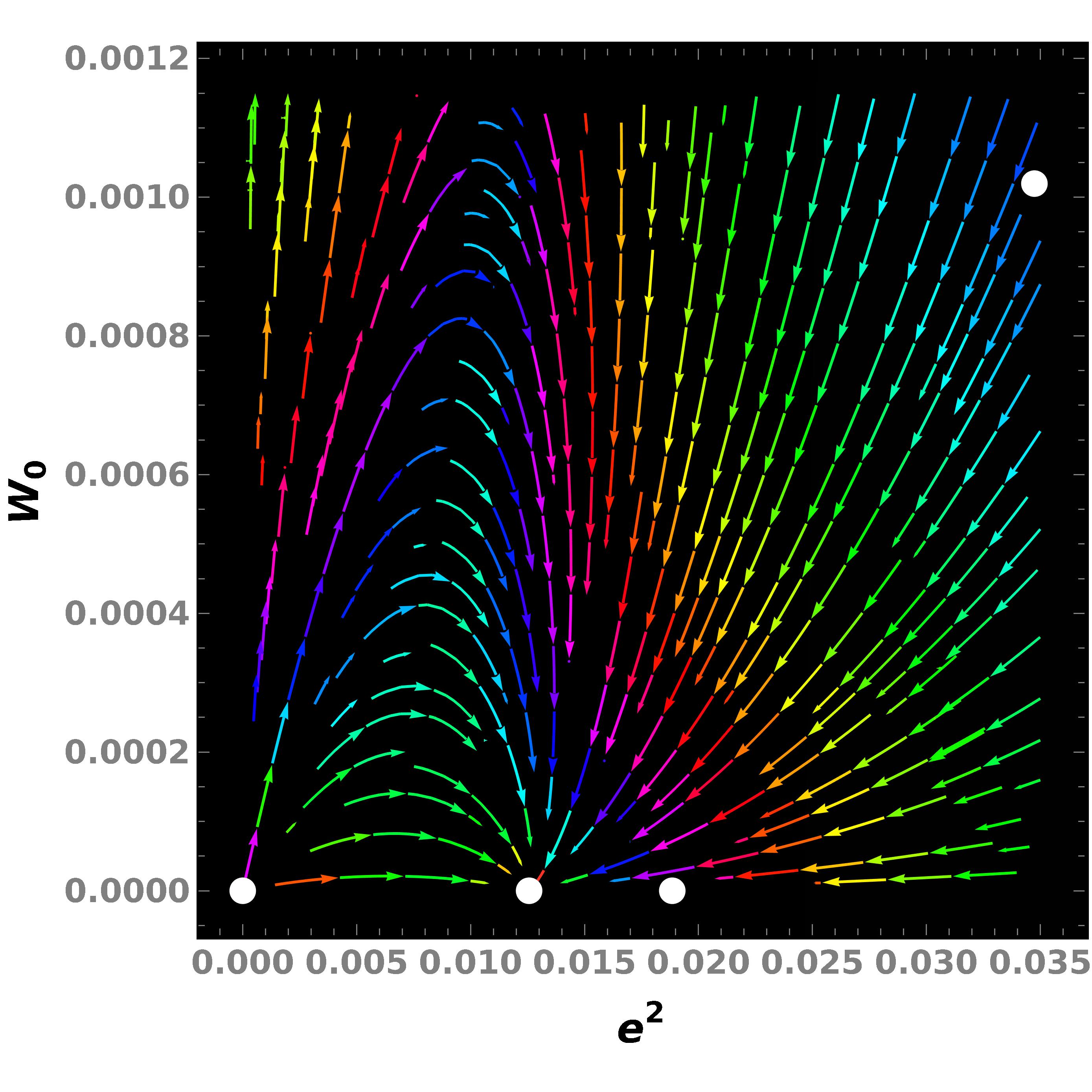
Expanding the coupling constants about each fixed point, we determine the stability matrix. Only for the fixed point $\left\{4\,\pi\,\varepsilon,0,0,0\right\}$, all eigenvalues of the stability matrix are negative, implying that it is the stable fixed point. The RG flows in three different planes are shown in Fig. 2. Hence, the marginal Fermi liquid fixed point survives in the presence of disorder.

To the counterterm action in Eq. (III.2), we now add the one required for the disorder. This is represented by

	$\displaystyle\mathcal{S}^{3d,c}_{\text{dis}}$	$\displaystyle=-\sum\limits_{a,b=1}^{n}\int d{k_{0}}\,d{p_{0}}\,\left(\prod\limits_{\eta=1}^{4}\int d^{3-\varepsilon}{\bf k}_{\eta}\right)\frac{\delta^{3-\varepsilon}\left({\bf k}_{1}+{\bf k}_{3}-{\bf k}_{2}-{\bf k}_{4}\right)}{\left(2\,\pi\right)^{2+3\left(2-\varepsilon\right)}}\left(A_{5}\,\bar{\mathcal{V}}\,\mu^{\varepsilon-1}+\frac{A_{6}\,{\mathcal{V}}\,\mu^{\varepsilon}}{|\mathbf{q}|}\right)$
		$\displaystyle\hskip 142.26378pt\times\left\{\tilde{\psi}_{a}^{{\dagger}}({k_{0}},\mathbf{k}_{1})\,{\tilde{\psi}_{a}}({k_{0}},\mathbf{k}_{2})\right\}\left\{\tilde{\psi}_{b}^{{\dagger}}({p_{0}},\mathbf{k}_{3})\,\tilde{\psi}_{b}({p_{0}},\mathbf{k}_{4})\right\},$
		$\displaystyle A_{n}\equiv\,Z_{n}-1=\sum_{\lambda=1}^{\infty}\frac{Z_{n,\lambda}}{\varepsilon^{\lambda}}\text{ with }n=5,6\,,$		(26)

where

$\displaystyle{\bar{\mathcal{V}}}_{B}=Z_{5}\,Z_{2}^{\varepsilon-3}\,{\bar{\mathcal{V}}}\,\mu^{\varepsilon-1}\,,\quad{\mathcal{V}}_{B}=Z_{6}\,Z_{2}^{\varepsilon-2}\,{\mathcal{V}}\,\mu^{\varepsilon}\,.$

(27)

We then get the corresponding renormalized action as

	$\displaystyle\mathcal{S}^{3d,ren}_{\text{dis}}$	$\displaystyle=-\sum\limits_{a,b=1}^{n}\int dk_{0_{B}}\,dp_{0_{B}}\,\left(\prod\limits_{\eta=1}^{4}\int d^{3-\varepsilon}{\bf k}_{\eta_{B}}\right)\frac{\delta^{3-\varepsilon}\left({\bf k}_{1_{B}}+{\bf k}_{3_{B}}-{\bf k}_{2_{B}}-{\bf k}_{4_{B}}\right)}{\left(2\,\pi\right)^{2+3\left(3-\varepsilon\right)}}\left(\bar{\mathcal{V}}_{B}+\frac{{\mathcal{V}}_{B}}{|\mathbf{q}_{B}|}\right)$
		$\displaystyle\hskip 142.26378pt\times\left\{\tilde{\psi}_{a}^{{\dagger}}({k_{0}}_{B},\mathbf{k}_{1_{B}})\,{\tilde{\psi}_{a}}({k_{0}}_{B},\mathbf{k}_{2_{B}})\right\}\left\{\tilde{\psi}_{b}^{{\dagger}}({p_{0}}_{B},\mathbf{k}_{3_{B}})\,\tilde{\psi}_{b}({p_{0}}_{B},\mathbf{k}_{4_{B}})\right\}.$		(28)

References

• Kennett et al. [2011] M. P. Kennett, N. Komeilizadeh, K. Kaveh, and P. M. Smith, Birefringent breakup of dirac fermions on a square optical lattice, Phys. Rev. A 83, 053636 (2011).
• Roy et al. [2012] B. Roy, P. M. Smith, and M. P. Kennett, Asymmetric spatial structure of zero modes for birefringent dirac fermions, Phys. Rev. B 85, 235119 (2012).
• Komeilizadeh and Kennett [2014] N. Komeilizadeh and M. P. Kennett, Instabilities of a birefringent semimetal, Phys. Rev. B 90, 045131 (2014).
• Dóra et al. [2011] B. Dóra, J. Kailasvuori, and R. Moessner, Lattice generalization of the dirac equation to general spin and the role of the flat band, Phys. Rev. B 84, 195422 (2011).
• Watanabe et al. [2011] H. Watanabe, Y. Hatsugai, and H. Aoki, Manipulation of the dirac cones and the anomaly in the graphene related quantum hall effect, Journal of Physics: Conference Series 334, 012044 (2011).
• Lan et al. [2011a] Z. Lan, N. Goldman, A. Bermudez, W. Lu, and P. Öhberg, Dirac-weyl fermions with arbitrary spin in two-dimensional optical superlattices, Phys. Rev. B 84, 165115 (2011a).
• Lan et al. [2011b] Z. Lan, A. Celi, W. Lu, P. Öhberg, and M. Lewenstein, Tunable multiple layered dirac cones in optical lattices, Phys. Rev. Lett. 107, 253001 (2011b).
• Bradlyn et al. [2016] B. Bradlyn, J. Cano, Z. Wang, M. G. Vergniory, C. Felser, R. J. Cava, and B. A. Bernevig, Beyond dirac and weyl fermions: Unconventional quasiparticles in conventional crystals, Science 353, aaf5037 (2016).
• Ezawa [2016] M. Ezawa, Pseudospin-32\frac{3}{2} fermions, type-ii weyl semimetals, and critical weyl semimetals in tricolor cubic lattices, Phys. Rev. B 94, 195205 (2016).
• Hsieh et al. [2014] T. H. Hsieh, J. Liu, and L. Fu, Topological crystalline insulators and dirac octets in antiperovskites, Phys. Rev. B 90, 081112 (2014).
• Chen et al. [2017] C. Chen, S.-S. Wang, L. Liu, Z.-M. Yu, X.-L. Sheng, Z. Chen, and S. A. Yang, Ternary wurtzite caagbi materials family: A playground for essential and accidental, type-i and type-ii dirac fermions, Phys. Rev. Materials 1, 044201 (2017).
• Roy et al. [2018] B. Roy, M. P. Kennett, K. Yang, and V. Juričić, From birefringent electrons to a marginal or non-fermi liquid of relativistic spin-1/21/2 fermions: An emergent superuniversality, Phys. Rev. Lett. 121, 157602 (2018).
• Nandkishore and Parameswaran [2017] R. M. Nandkishore and S. A. Parameswaran, Disorder-driven destruction of a non-fermi liquid semimetal studied by renormalization group analysis, Phys. Rev. B 95, 205106 (2017).
• Mandal and Nandkishore [2018] I. Mandal and R. M. Nandkishore, Interplay of coulomb interactions and disorder in three-dimensional quadratic band crossings without time-reversal symmetry and with unequal masses for conduction and valence bands, Phys. Rev. B 97, 125121 (2018).
• Dalidovich and Lee [2013] D. Dalidovich and S.-S. Lee, Perturbative non-fermi liquids from dimensional regularization, Phys. Rev. B 88, 245106 (2013).
• Mandal and Lee [2015] I. Mandal and S.-S. Lee, Ultraviolet/infrared mixing in non-fermi liquids, Phys. Rev. B 92, 035141 (2015).
• Mandal [2016] I. Mandal, UV/IR Mixing In Non-Fermi Liquids: Higher-Loop Corrections In Different Energy Ranges, Eur. Phys. J. B 89, 278 (2016).
• Mandal [2020] I. Mandal, Critical fermi surfaces in generic dimensions arising from transverse gauge field interactions, Phys. Rev. Research 2, 043277 (2020).
• Note [1] There are two possible contractions (matching one ψ~\tilde{\psi}^{{\dagger}} with one ψ~\tilde{\psi}) of the interaction term in Eq. (2\@@italiccorr) that gives the fermion self-energy. In the real space, the ‘Hartree’ contractions are of the form ψ(t,x)ψ(t,x)ψ(t,x)ψ(t,x)\langle\psi^{{\dagger}}(t,x)\,\psi(t,x)\rangle\,\psi^{{\dagger}}(t^{\prime},{x^{\prime}})\,\psi(t^{\prime},{x^{\prime}}), and correspond to tadpole diagrams. These simply shift the overall chemical potential, and can be ignored (since we assume that the renormalized chemical potential is at the band-crossing point). However, the ‘exchange’ contractions contribute (cannot be ignored). These latter contributions are of the form ψ(t,x)ψ(t,x)ψ(t,x)ψ(t,x)\langle\psi^{{\dagger}}(t,x)\,\psi(t^{\prime},{x^{\prime}})\rangle\,\psi^{{\dagger}}(t^{\prime},{x^{\prime}})\,\psi(t,x), and ψ(t,x)ψ(t,x)ψ(t,x)ψ(t,x)\langle\psi^{{\dagger}}(t^{\prime},x^{\prime})\,\psi(t,{x})\rangle\,\psi^{{\dagger}}(t,{x})\,\psi(t^{\prime},x^{\prime}). Due to two ways of contractions, we get a factor of 2.
• Pimenov et al. [2018] D. Pimenov, I. Mandal, F. Piazza, and M. Punk, Non-fermi liquid at the fflo quantum critical point, Phys. Rev. B 98, 024510 (2018).
• Eberlein et al. [2016] A. Eberlein, I. Mandal, and S. Sachdev, Hyperscaling violation at the ising-nematic quantum critical point in two-dimensional metals, Phys. Rev. B 94, 045133 (2016).
• Mandal [2017] I. Mandal, Scaling behaviour and superconducting instability in anisotropic non-fermi liquids, Annals of Physics 376, 89–107 (2017).
• Mandal and Ziegler [2021] I. Mandal and K. Ziegler, Robust quantum transport at particle-hole symmetry, EPL (Europhysics Letters) 135, 17001 (2021).
• Mandal and Freire [2021] I. Mandal and H. Freire, Transport in the non-fermi liquid phase of isotropic luttinger semimetals, Phys. Rev. B 103, 195116 (2021).
• Freire and Mandal [2021] H. Freire and I. Mandal, Thermoelectric and thermal properties of the weakly disordered non-fermi liquid phase of luttinger semimetals, Physics Letters A 407, 127470 (2021).
• Roy and Juričić [2020] B. Roy and V. Juričić, Relativistic non-fermi liquid from interacting birefringent fermions: A robust superuniversality, Phys. Rev. Research 2, 012047 (2020).
• Mandal [2018] I. Mandal, Fate of superconductivity in three-dimensional disordered luttinger semimetals, Annals of Physics 392, 179–195 (2018).