∎
State Key Lab of Intelligent Technologies and Systems
Tsinghua National Laboratory for Information Science and Technology(TNList)
Beijing. 100084. P.R.China
22email: [email protected] 33institutetext: Kun Chen 44institutetext: Department of Statistics
University of Connecticut
Storrs, CT 06269, USA
44email: [email protected] 55institutetext: Ming Lin 66institutetext: Department of Computational Medicine and Bioinformatics
University of Michigan
Ann Arbor, MI 48109, USA
66email: [email protected] 77institutetext: Changshui Zhang 88institutetext: Department of Automation, Tsinghua University
State Key Lab of Intelligent Technologies and Systems
Tsinghua National Laboratory for Information Science and Technology(TNList)
Beijing. 100084. P.R.China
88email: [email protected] 99institutetext: Fei Wang 1010institutetext: Department of Healthcare Policy and Research
Cornell University
New York City. NY 10065. USA
1010email: [email protected]
Robust Finite Mixture Regression for Heterogeneous Targets
Abstract
Finite Mixture Regression (FMR) refers to the mixture modeling scheme which learns multiple regression models from the training data set. Each of them is in charge of a subset. FMR is an effective scheme for handling sample heterogeneity, where a single regression model is not enough for capturing the complexities of the conditional distribution of the observed samples given the features. In this paper, we propose an FMR model that 1) finds sample clusters and jointly models multiple incomplete mixed-type targets simultaneously, 2) achieves shared feature selection among tasks and cluster components, and 3) detects anomaly tasks or clustered structure among tasks, and accommodates outlier samples. We provide non-asymptotic oracle performance bounds for our model under a high-dimensional learning framework. The proposed model is evaluated on both synthetic and real-world data sets. The results show that our model can achieve state-of-the-art performance.
Keywords:
Finite Mixture RegressionMixed-type ResponseIncomplete TargetsAnomaly DetectionTask Clustering1 Introduction
Regression modeling, which refers to building models to learn conditional relationship between output targets and input features on some training samples, is a fundamental problem in statistics and machine learning. Some classical regression modeling approaches include least square regression, logistic regression and Poisson regression; see, e.g., Bishop (2006), Kubat (2015), Fahrmeir et al (2013) and the references therein.
The aforementioned classic approaches usually train a single model of a single target over the entire data set. However, real-world problems can be much more complicated. In particular, the needs of utilizing high-dimensional features, population heterogeneity, and multiple interrelated targets are among the most prominent complications. To handle high-dimensional data, the celebrated regularized estimation approaches have undergone exciting developments in recent years; see, e.g., Fan and Lv (2010) and Huang et al (2012). In the presence of population heterogeneity, the samples may form several distinct clusters corresponding to mixed relationships between the targets and the features. A popular modeling strategy in such a scenario is the Finite Mixture Regression (FMR) (McLachlan and Peel, 2004), which is capable of adaptively learning multiple models, each of which is responsible for one subset/cluster of the data. FMR models have been widely used in market segmentation studies, patients’ disease progression subtyping, motif gene-expression research, etc.; see, e.g., Städler et al (2010), Khalili (2011), Khalili and Chen (2007), Do˘ru and Arslan (2017), and the references therein. The problem of joint learning for multiple targets is usually referred to as Multi-Task Learning (MTL) in machine learning or multivariate learning in statistics; see, e.g., Argyriou et al (2007a), Argyriou et al (2007b), Chen et al (2011), and Gong et al (2012b). We stress that the main definition of MTL considers tasks that do not necessarily share the same set of samples (and features), and that this paper focuses on a special case of MTL, where the multivariate outcomes are collected from the same set of samples and share the same set of features, whose reason will be explained later. There have also been multi-task FMR models, e.g., Wedel and DeSarbo (1995), Xian Wang et al (2004), Kyung Lim et al (2016) and Bai et al (2016), which mainly built on certain multivariate probability distribution such as Gaussian distribution or multivariate distribution.
Thus far, a comprehensive study on multi-task mixture-regression modeling with high-dimensional data is still lacking. To tackle this problem for handling real-world applications, there remain several challenges and practical concerns.
-
•
Task Heterogeneity. Current MTL approaches usually assume that the targets are of the same type. However, it is common that the multiple targets are of different types, such as continuous, binary, count, etc., which we refer to as task heterogeneity. For example, in anesthesia decision making (Tan et al, 2010), the anesthesia drugs will have impacts on multiple indicators of an anesthesia patient, such as anesthesia depth, blood pressures, heart rates, etc. The anesthesiologist needs to consider all those different aspects as well as their intrinsic dependence before making the decision.
-
•
Task Integration. As in the anesthesiology example, the multiple tasks are typically inter-related to each other, and the potential benefit from a MTL approach needs to be realized through properly exploring and taking advantage of these relationships. In existing high-dimensional MTL approaches, the tasks are usually integrated by assuming certain shared conditional mean structures between the targets and the features. The problem is more difficult in the presence of both task and population heterogeneities.
-
•
Task Robustness. Similar to the idea in the robust MTL approaches (Passos et al, 2012; Gong et al, 2012a; Chen et al, 2011), it is not always the case that jointly considering all tasks by assuming certain shared structures among them would be helpful. Certain tasks, referred to as anomaly tasks, may not follow the assumed shared structure and thus can ruin the overall model performance. More generally, tasks may even cluster into groups with different shared structures.
In this paper, we propose a novel method named HEterogeneous-target Robust MIxTure regression (Hermit), to address the above challenges in a unified framework. Here we explain that we mainly consider the setting, where the multivariate outcomes are collected from the same set of samples and share the same set of features because our main objective is to learn potentially shared sample clusters and feature sets among tasks. Rigorous theoretical analysis and performance guarantees are provided. It is worthwhile to highlight the key aspects of our approach as follows.
-
•
Our method handles mixed type of targets simultaneously. Each target follows an exponential dispersion family model (Jorgensen, 1987), so that multiple different types of targets, e.g., continuous, binary, and counts, can be handled jointly. The tasks are naturally integrated through sharing the same clustering structure arising from population heterogeneity. Our theory allows Hermit to cover sub-exponential distributions, including the commonly-encountered Bernoulli, Poisson and Gaussian as special cases.
-
•
Our method imposes structural constraints in each mixture component of Hermit, to deal with the curse of dimensionality and at the same time further take advantage of the interrelationship of the tasks. In particular, the group penalization is adopted to perform shared feature selection among tasks within each mixture component.
-
•
Our method adopts three strategies for robustness. First, we adopt a mean-shift regularization technique (She and Chen, 2017) to detect the outlier samples automatically and adjust for its outlying effects in model estimation. The second strategy measures discrepancy of different conditional distributions to detect anomaly tasks. The third strategy measures similarity between each pair of tasks to discover a clustered structure among tasks. Moreover, our model can work with incomplete data and impute entry-wise missing values in the multiple targets.
The aforementioned key elements, e.g., multi-task learning, sample clustering, shared feature selection, and anomaly detection, are integrated in a unified mixture model setup, so that they can benefit from and reinforce each other. A generalized Expectation-Maximization (GEM) (Neal and Hinton, 1998) algorithm is developed to conduct model estimation efficiently. For theoretical analysis, we generalize the results of Städler et al (2010) to establish non-asymptotic oracle performance bounds for Hermit under a high-dimensional learning framework. This is not trivial due to the non-convexity (due to the population heterogeneity) and the target heterogeneity of the problem.
The rest of this paper is organized as follows. Section 2 provides a brief review of the background and the related works to our method. Section 3 presents the details of the proposed Hermit model and the computational algorithm. Section 4 discusses several extensions of our method. Section 5 shows the theoretical analysis. The empirical evaluations are presented in Section 6, followed by the discussions and conclusions in Section 7.
2 Background & Related Work
Let be the output target and the input feature vector. GLMs (Nelder and Baker, 1972) postulate that the conditional probability density function of given is
where with being the regression coefficient vector, is a dispersion parameter, and are known functions whose forms are determined by the specific distribution. Here we use to denote the collection of all the unknown parameters, i.e., . Least square regression, logistic regression and Poisson regression are all special cases of GLMs. In the presence of population heterogeneity, a standard finite mixture model of GLM postulates that the conditional probability density function of given is
where with being the regression coefficient vector for the th mixture component, and with . So FMR model assumes that there are sub-populations, each of which admits a different conditional relationship between and .
McLachlan and Peel (2004) introduced finite mixture of GLM models. Bartolucci and Scaccia (2005) considered a special case that are different only in their first entries. Khalili and Chen (2007) discussed using sparse penalties such as Lasso and SCAD to perform feature selection for FMR models and showed asymptotic properties of the penalized estimators. Städler et al (2010) reparameterized the finite mixture of Gaussian regression model and used penalization to achieve bounded log-likelihood and consistent feature selection. For multiple targets, Wedel and DeSarbo (1995) proposed finite mixture of GLM models with multivariate targets. These methods only consider the univariate-outcome case. Weruaga and Vía (2015) proposed multivariate Gaussian mixture regression and used penalty for sparseness of parameters. Besides mixture of GLMs, there have been many works on mixture of other continuous distributions such as and Laplace distributions, mainly motivated by the needs of robust estimation for handling heavy tailed or skewed continuous distribution; see, e.g., Xian Wang et al (2004); Do˘ru and Arslan (2017); Alfò et al (2016); Doğru and Arslan (2016); Kyung Lim et al (2016); Bai et al (2016). However, these methods assume that the targets are of the same type, and only consider interrelationship among tasks with continuous outcomes. Additionally, they all assumed that their FMR model is shared by all the tasks.
In MTL, Kumar and Daumé III (2012), Passos et al (2012), Gong et al (2012a), Chen et al (2011), Jacob et al (2009), Chen et al (2010) and He and Lawrence (2011) proposed to tackle the problem that different groups of tasks share different information, providing methods to handle anomaly tasks, clustered structure or graph-based structure among tasks. Yang et al (2009) proposed a multi-task framework to jointly learn tasks with output types of Gaussian and multinomial. Zhang et al (2012) proposed a multi-modal multi-task model to predict clinical variables for regression and categorical variable for classification jointly. Li et al (2014) proposed a heterogeneous multi-task learning framework to learn a pose-joint regressor and a sliding window body-part detector in a deep network architecture simultaneously. Nevertheless, these MTL methods cannot handle the heterogeneity of conditional relationship between features and targets.
By contrast, the proposed FMR framework Hermit is effective for handling sample heterogeneity with mixed type of tasks whose interrelationship are harnessed by structural constraints. Non-asymptotic theoretical guarantees are provided. It also handles anomaly tasks or clustered structure among tasks, for the case that not all the tasks share the same FMR structure.
3 HEterogeneous-target Robust MIxTure regression
In this section, we first present the formulation of the main Hermit model, followed by penalized likelihood estimators with sparse constraint and structural constraint, respectively. We then introduce the associated optimization procedures, and describe how to perform sample clustering and make imputation of the missing/unobserved outcomes on incomplete multi-target outcomes based on the main model. Hyper-parameter tuning is discussed at last. Various extensions of the main methodology, including strategies to handle anomaly tasks or clustered tasks, will be introduced in Section 4.
3.1 Model Formulation and Estimation Criterion
Let be the output/target data matrix and the input/feature data matrix, consisting of independent samples , . As such, there are different targets with a common set of features. We allow to contain missing values at random; define be the collection of indices of observed outcome in the th sample (), for .
To model multiple types of targets, such as continuous, binary, count, etc., we allow to potentially follow different distributions in the exponential-dispersion family, for each . Specifically, we assume that given , the joint probability density function of is
| (1) |
where
is the natural parameter for the th sample of the th target in the th mixture component, is the dispersion parameter of the th target in the th mixture component, and the functions are determined by the specific distribution of the th target. Here, the key assumption is that the tasks all correspond to the same cluster structure (e.g., the tasks all have clusters) determined by the underlying population heterogeneity; given the shared cluster label (e.g., ), the tasks within each mixture component then become independent of each other (depicted by the product of their probability density functions). As such, by allowing cluster label sharing, the model provides an effective way to genuinely integrate the learning of the multiple tasks.
Following the setup of GLMs, we assume a linear structure in the natural parameters, i.e.,
| (2) |
where is the regression coefficient vector of the th response in the th mixture component. Since is possibly of high dimensionality, the s are potentially sparse vectors. For example, when the s for share the same sparsity pattern, the tasks share the same set of relevant features within each mixture component. For , write and . Also write . Let collecting all the unknown parameters, with the parameter space given by where .
The data log-likelihood of the proposed model is
| (3) |
The missing values in simply do not contribute to the likelihood, which follows the same spirit as in matrix completion (Candès and Recht, 2009). The proposed model indeed possesses a genuine multivariate flavor, as the different outcomes share the same underlying latent cluster pattern of the heterogeneous population. We then propose to estimate by the following penalized likelihood criterion:
| (4) |
where is some certain penalty term on the regression coefficients with being a tuning parameter.
We thus name our proposed method the HEterogeneous-target Robust MIxTure regression (Hermit). The can be flexibly chosen based on specific needs of feature selection. The first sparse penalties adopted by our model is the norm (lasso-type) penalty,
| (5) |
where is the tuning parameter, is the entry-wise norm, and s are the penalty weights with being a pre-specified constant. Here the penalty also depends on the unknown mixture proportions ; when the cluster sizes are expected to be imbalanced, using this weighted penalization with some is preferred (Städler et al, 2010). This entry-wise regularization approach allows the tasks to have independent set of relevant features. Alternatively, in order to enhance the integrative learning and potentially boost the performance of clustering, it could be beneficial to encourage the internal similarity within each sub-population. Then certain group-wise regularization of the features could be considered, which are widely adopted in multi-task learning. In particular, we consider a component-specific group sparsity pattern to achieve shared feature selection among different tasks, in which the group norm penalty is used (Gong et al, 2012a; Jalali et al, 2010),
| (6) |
where denotes the sum of the row norms of the enclosed matrix, and the weights are constructed as in (5). The shared feature set in each sub-population can be used to characterize the sub-population and render the whole model more interpretable.
3.2 Optimization
We propose a generalized EM (GEM) algorithm (Dempster et al, 1977) to solve the minimization problem in (4). For each , define be a set of latent indicator variables, where if the th sample belongs to the th component of the mixture model (1) and otherwise. So , . These indicators are not observed since the cluster labels of the samples are unknown. Let denote the collection of all the indicator variables. By treating as missing, the EM algorithm proceeds by iteratively optimizing the conditional expectation of the complete log-likelihood criterion.
The complete log-likelihood is given by
where , for , and . The conditional expectation of the penalized complete negative log-likelihood is then given by
where can be any of the penalties in (5) or (6). It is easy to show that deriving boils down to the computation of , which admits an explicit form.
The EM algorithm proceeds as follows. Let be some given initial values. We repeat the following steps for , until convergence of the parameters or the pre-specified maximum number of iteration is reached.
E-Step: Compute . For ,
| (7) |
M-Step: Minimize .
a) Update by solving
b) Update .
For the problem in a), Städler et al (2010) proposed a procedure to lower the objective function by a feasible point, and we find that simply setting is good enough. For the problem in b), we use an accelerated proximal gradient (APG) method introduced in Nesterov et al (2007) with the maximum number of iteration of . The update steps by proximal operators correspond to the chosen penalty form. For the entry-wise norm penalty in (5),
| (8) |
where denotes entry-wise product, , denotes the step size, and denotes the update direction of determined by APG. For the group norm penalty in (6),
where denotes the th column of . We adopt the active set algorithm in Städler et al (2010) to speed up the computation.
The time complexity of our algorithm using the speed up technique is with being the number of non-zero parameters. The algorithm performs well in practice, and we have not observed any convergence issues in our extensive numerical studies.
3.3 Clustering of Samples & Imputation of Missing Targets
From the model estimation, we can get estimates of both the conditional probabilities and the conditional means , where . Specifically, the conditional probabilities can be estimated by which corresponds to (7), taking . The conditional expectations can be estimated as .
For clustering the samples, we adopt the Bayes rule, i.e., for ,
| (9) |
Following the idea of Jacobs et al (1991), we propose to make imputation for the missing outcomes by
| (10) |
3.4 Tuning Hyper-Parameters
Unless otherwise specified, all the hyper-parameters, including regularization coefficients s and the number of clusters , are tuned to maximize the data log-likelihood in (3) on the held-out validation data set. In other words, we fit models on training data with different specific hyper-parameter settings, and then the optimal model is chosen as the one that gives the highest log-likelihood in (3) of the held-out validation data set. This approach is fairly standard and has been widely used in existing works (Städler et al, 2010). Moreover, cross validation and various information criteria (Bhat and Kumar, 2010; Aho et al, 2014) can also be applied to determine hyper-parameters.
4 Extensions
We provide several extensions of the proposed Hermit approach described in Section 3, including robust estimation against outlier samples, handling anomaly tasks or clustered structure among tasks, and modeling mixture probabilities for feature-based prediction.
4.1 Robust Estimation
To perform robust estimation for parameters in the presence of outlier samples, we propose to adopt the mean shift penalization approach (She and Owen, 2011). Specifically, we extend the natural parameter model to the following additive form,
| (11) |
where is a case-specific mean shift parameter to capture the potential deviation from the linear model. Apparently, when is allowed to vary without any constraint, it can make the model fit as perfect as possible for every . The merit of this approach is realized by assuming certain sparsity structure of the s, so that only a few of them have nonzero values corresponding to anomalies. Write for , and . We can then conduct joint model estimation and outlier detection by extending (4) to
| (12) |
where, for example, the penalty on can be chosen as the group penalty,
| (13) |
so that entries of are nonzero for only a few data samples.
The proposed GEM algorithm can be readily extended to handle the inclusion of , for which we omit the details.
4.2 Handling Anomaly Tasks
Besides outlier samples, certain tasks, referred to as anomaly tasks, may not follow the assumed shared structure and thus can ruin the overall model performance. To handle anomaly tasks, though it is also intuitive to adopt the approach above, our numerical study suggests that its performance is sensitive to the tuning parameters. Here, we adopt the idea of Koller and Sahami (1996) , by utilizing the estimated conditional probabilities to measure how well a task is concordant with the estimated mixture structure. Consider the th task. The main idea is to measure the discrepancy between , the conditional probability based on data from all observed targets, and , the conditional probability based on only the th task. If th task is an anomaly task, it is expected that the two conditional probabilities would differ more from each other (Koller and Sahami, 1996; Law et al, 2002).
For , , let
| (14) | ||||
Define and . Then we define the concordant score of the th task as
| (15) |
where is the widely used Kullback-Leibler divergence (Cover and Thomas, 2012).
The tasks can then be ranked based on their concordant scores. As such, the detection of anomaly tasks boils down to a one-dimensional outlier detection problem. After anomaly tasks are detected, their FMR models can be built.
4.3 Handling Clustered Structure among tasks
In practice, tasks may be clustered into groups such that each task group has its own model structure. Here we assume that each cluster of tasks shares a FMR structure defined in (1), and propose to construct a similarity matrix to discover the potential cluster pattern among tasks.
We consider a two-stage strategy. First, each task learns a FMR model on the training data independently with the same pre-fixed . Then we get for all , where
and and are the latent variables and the estimated prior probabilities of the th task, respectively.
Second, we adopt Normalized Mutual Information (NMI) (Strehl and Ghosh, 2002a) to measure the similarity between each pair of tasks. We choose NMI instead of Kullback-Leibler divergence because NMI can handle the case that the orders of clusters of two -cluster structures are different. Specifically, given two methods to estimate latent variables, which are denoted by method and method , let and denote the estimated probability of latent variables of method and method , respectively, where for . NMI is defined as
| (16) |
where denotes the mutual information between such that
Following Strehl and Ghosh (2002a), we approximate , and by
As such, given the estimated models for the th and the th task, respectively, we treat and as and , respectively, for . Then NMI between each pair of tasks are computed by (16). We note that for simplicity we set the pre-fixed to be the same, but in general can be different for different tasks by the definition of Mutual Information.
Given the similarity between each pair of tasks, any similarity-based clustering method can be applied to cluster tasks into groups. Empirically, the performance of task clustering is not sensitive to the pre-fixed . As such, we set the pre-fixed to be in this paper. We then apply the proposed Hermit approach separately for each task group.
4.4 Modeling Mixture Probabilities
In real-applications, one may require to use only to infer the latent variables and then to predict , for . Here we further extend our method following the idea of Mixture-Of-Experts (MOE) (Yuksel et al, 2012) model; the only modification is that in (1) is assumed to be function of , for .
To be specific, let collect regression coefficient vectors for a multinomial linear model. We assume that given , the joint probability density function of in (1) is replaced by
where
| (17) |
is referred to as the gating probability. All the other terms are defined the same as in (1).
Let , with the parameter space The data log-likelihood of the MOE model is
| (18) |
The model estimation is conducted by extending (4) to
| (19) |
where, for example, the penalty on can be chosen as the lasso type penalty,
| (20) |
5 Theoretical Analysis
We study the estimation and variable selection performance of Hermit under the high-dimensional framework with . Both and , on the other hand, are considered as fixed. This is because usually, the number of interested targets and the number of desired clusters are not large in many real problems. Here we only present the setup and the main results on non-asymptotic oracle inequalities to bound the excess risk and false selection, leaving detailed derivations in the Appendix. Our results generalize Städler et al (2010) to cover mixture regression models with 1) multivariate, heterogeneous (mixed-type) and incomplete response and 2) shared feature grouping sparse structure. This is not trivial due to the non-convexity and the triple heterogeneity of the problem. It turns out that additional condition on the tail behaviors of the conditional density is required. Fortunately, the required conditions are still satisfied by a broad range of distributions.
5.1 Notations and Conditions on the Conditional Density
We firstly introduce some notations. Denote the regression parameters that are subject to regularization by , where is the vectorization operator. The other parameters in the mixture model are denoted by , where is entry-wisely applied. Denote the true parameter by to be estimated under the FMR model defined in (1) and (2). In the sequel, we always use subscripts “” to represent parameters or structures under the true model. To study sparsity recovery, denote the set of indices of non-zero entries of the true parameter by . We use to indicate that the inequality holds up to some multiplicative numerical constants. To focus on the main idea, we consider the case of in the following analysis.
We define average excess risk for fixed design points based on Kullback-Leibler divergence as
where is defined in (1).
To impose the conditions on , denote , where , and denote . As such, we may write , , and .
Without loss of much generality, the model parameters are assumed to be in a bounded parameter space for a constant :
| (23) |
We present the following conditions on .
Condition 1
For some function , for ,
Condition 2
For a constant , and some constants depending , and for , we assume for ,
where , and denotes the indicator function.
Condition 3
It holds that,
where is a constant, is the smallest eigenvalue of a symmetric, positive semi-definite matrix and for , is the Fisher information matrix such that
The first condition follows from Städler et al (2010), which aims to bound with known , for . The second condition is about the tail behaviors of . The third condition depicts the local convexity of at the point . Condition 1 and 2 can cover a broad range of distributions for , including but not limited to mixture of sub-exponential distributions, such as our proposed Hermit model with known dispersion parameters, c.f., Lemma 1.
Lemma 1
The following two quantities will be used.
| (24) |
where are the same constants as in Condition 2. More specifically, we choose for Gaussian, Bernoulli and Poisson task, respectively.
5.2 Results for Lasso-Type Estimator
Consider first the penalized estimator defined in (4) with the penalty in (5). Following Bickel et al (2009) and Städler et al (2010), we impose the following restricted eigenvalue condition on the design.
Condition 4
(Restricted eigenvalue condition). For all satisfying , it holds that for some constant ,
Theorem 1
Theorem 1 suggests that the average excess risk has a convergence rate of the order , by taking and using and as defined in (24). Also, the degree of false selection measured by converge to zero at rate .
Similar to Städler et al (2010), under weaker conditions without the restricted eigenvalue assumption on the design, we still achieve the consistency for the average excess risk.
5.3 Results for Group-Lasso Type Estimator
Consider the following general form of the group penalty,
| (27) |
where are index collections such that for and equals the universal set of indices of , i.e., is the th group of . denotes the Frobenius norm and here for , . This penalty form generalizes the row-wise group sparsity in (6).
Denote and where is the th group of . Now denote by the size of , with some abuse of notation. We impose the following group-version restricted eigenvalue condition.
Condition 5
For all satisfying
it holds that for some constant ,
Theorem 3
Consider the Hermit model in (1) with , and consider the penalized estimator (4) with the group penalty in (27).
(a) Assume conditions 1-3 and 5 hold. Suppose , and take for some constant . For some constant and large enough , with the following probability we have
(b) Assume conditions 1-3 hold (without condition 5), and assume
as . Let for some sufficiently large. Then for some constant and large enough , with the following probability we have
So the average excess risk has a convergence rate of , and the degree of false group selection, as measured by , converges to zero at rate . The estimator in (4) using other group penalties such as (6) are special cases, so the results of Theorem 3 still apply.
Remark. Our results can be extended to the mean-shifted natural parameter model as in (11), with a modified restricted eigenvalue condition. See the Appendix for some details.
6 Experiments
In this section, we present empirical studies on both synthetic and real-world data sets.
6.1 Methods for Comparison
We evaluate the following versions of the proposed Hermit approach.
(1) Single task learning (Single): It is a special case of the Hermit estimator (4) with (5), where each task is learned separately.
(2) Separately learning (Sep): It is a special case of the Hermit estimator (4) with (5), where each type (Gaussian, Bernoulli or Poisson) of tasks is learned separately.
(3) Mixed learning with entry-wise sparsity (Mix): It is the proposed Hermit estimator (4) with (5) where all the tasks are jointly learned. To compare with Sep, we allow different tuning parameters for different types of outcomes.
(5) Mixed learning Mixture-Of-Experts model with entry-wise sparsity (Mix MOE): It is the proposed Hermit estimator (19) with (5) and (20).
(6) Mixed learning Mixture-Of-Experts model with group sparsity (Mix MOE GS): It is the proposed Hermit estimator (19) with (6) and (20).
Besides the above FMR methods, we also evaluate several non-FMR multi-task methods below for comparison, some of which handle certain kinds of heterogeneities, such as anomaly tasks, clustered tasks and heterogeneous responses. Since they are non-FMR, they learn a single regression coefficient matrix .
-
•
LASSO: -norm multi-task regression with as penalty. Each type of tasks are learned independently. It is a special case of Sep when pre-fixed .
-
•
Sep L2: ridge multi-task regression with as penalty. Each type of tasks are learned independently.
-
•
Group LASSO: -norm multi-task regression with as penalty (Yang et al, 2009), which handles heterogeneous responses, and is a special case of Mix GS when pre-fixed .
-
•
TraceReg: trace-norm multi-task regression (Ji and Ye, 2009).
-
•
Dirty: dirty model multi-task regression with as penalty (Jalali et al, 2010), handling entry-wise heterogeneity in comparing with Group LASSO.
-
•
MSMTFL: multi-stage multi-task feature learning (Gong et al, 2012b) whose penalty is , where denotes the th row of . It also handles entry-wise heterogeneity in comparing with Group LASSO.
-
•
SparseTrace: multi-task regression, learning sparse and low-rank patterns with as penalty (Chen et al, 2012a), handling entry-wise heterogeneity in comparing with TraceReg, where denotes the nuclear norm of the enclosed matrix.
-
•
rMTFL: robust multi-task feature learning with as penalty (Gong et al, 2012a), handling anomaly tasks comparing with Group LASSO.
-
•
RMTL: robust multi-task regression with as penalty (Chen et al, 2011), handling anomaly tasks comparing with TraceReg.
-
•
CMTL: clustered multi-task learning (Zhou et al, 2011), handling clustered tasks.
-
•
GO-MTL: multi-task regression, handling overlapping clustered tasks (Kumar and Daumé III, 2012).
6.2 Experimental Setting
In our experiments, for the E-step of GEM, we follow Städler et al (2010) to initialize . For the M-step, we initialize the entries of from . We fix for Gaussian tasks, and set . In the APG algorithm, step size is initialized by the Barzilai-Borwein rule (Barzilai and Borwein, 1988) and updated by the TFOCS-style backtracking (Becker et al, 2011).
We terminate the APG algorithm with maximum iteration step or when the relative -norm distance of two consecutive parameters is less than . We terminate the GEM with maximum iteration step , or when the relative change of two consecutive is less than or when the relative -norm distance of two consecutive parameters is less than .
In the experiments on both simulated and real-world data sets, we partition the entire data set into three parts: a training set for model fitting, a validation set for tuning hyper-parameters and a testing set for testing the generalization performance of the selected models. The only exception is Section 6.4.1, where we do not generate testing data sets because the models are evaluated by comparing the estimation results to the ground truth.
In hyper-parameter tuning, the regularization parameters, i.e., s, are tuned from , and the number of clusters are tuned from . Hyper-parameters of the baseline methods are tuned according to the descriptions in their respective references.
All the experiments are replicated 100 times under each model setting.
6.3 Evaluation Metrics
The prediction of latent variable is evaluated by Normalized Mutual Information (NMI) (Strehl and Ghosh, 2002b; Fern and Brodley, 2003; Strehl and Ghosh, 2002a). In detail, we compute NMI scores by (16), treating estimated conditional probabilities defined in (14) and the ground truth latent variables as and , respectively.
For feature selection, firstly, the estimated components are reordered to make the best match with the true components. Then feature selection is evaluated by Area Under the ROC Curve (AUC) which is measured by the Wilcoxon-Mann-Whitney statistic provided by Hanley and McNeil (1982). Concretely, absolute values of vectorized estimated regression parameters, i.e., , and binarized vectorized ground truth regression parameters, i.e., , are used as inputs to AUC, where denotes the ground truth regression parameter and is the vectorization operator.
In order to show the existence of mixed relationships between features and targets, imputation performance for incomplete targets is used to compare FMR methods with non-FMR MTL methods. Concretely, the goal is to predict one-half randomly chosen targets. The other half targets are allowed to be used. FMR methods use the other half targets to compute conditional probabilities and make prediction as stated in Section 3.3. Non-FMR MTL methods perform feature-based prediction.
Feature-based prediction performances are also compared between non-FMR MTL methods and our MOE methods, where only features are allowed to use to predict testing targets. For this case, the goal is to predict all the targets.
For target prediction, Gaussian outcomes are evaluated by nMSE (Chen et al, 2011; Gong et al, 2012a) which is defined as the mean of each task’s mean squared error (MSE) divided by the variance of its target vector. Bernoulli outcomes are evaluated by average AUC (aAUC), which is defined as the mean AUC of each task. For Poisson tasks, we firstly compute the logarithms of outcomes, then use nMSE for evaluation.
Since our objective functions in (4) and (19) are non-convex, estimated parameters may correspond to local minimums of the objective functions. Therefore, we try different initializations and report the results ranking the best 20% on the validation data set out of the 100 replications to avoid the results that may be stuck at local minimums, suggesting that one can always select any result within the best 20%.
6.4 Simulation
6.4.1 Latent Variable Prediction and Feature Selection
We consider both low dimensional case and high dimensional case for latent variable prediction and feature selection. For the low-dimensional case, we set the number of samples , feature dimension , number of non-zero features (sparsity) , and the number of tasks (responses) . The data set includes Gaussian tasks, Bernoulli tasks, and Poisson tasks. The number of latent components . For , in the th component, the first row (biases) and the th to the th row (a block of rows) of the true are non-zero (to let different components have different sets of features). Non-zero parameters in are in the range of except that those of Poisson tasks are in the range of . The biases are all set to except that those of Poisson tasks are set to . For Gaussian tasks, all s are set to . The entries of are drawn from with the first dimension being . . Validation data is independently generated likewise and has samples. For the high-dimensional case, we set , and . The data set includes Gaussian tasks, Bernoulli tasks, and Poisson tasks. Other settings are the same as in the low-dimensional case. We set the pre-fixed to be equal to the true . For targets of training data, we have tried different missing rates, which are in the range of . We compare the performances of s estimated by Single, Sep, Mix, Mix GS, respectively, with that of (denoted by “True”).
The results are shown in Fig 1. The horizontal axis is the missing rates. Intuitively, larger missing rates may result in worse performances due to fewer data samples. Single provides poor results and is not sensitive to missing rate, because (1) data samples are deficient for single-task learning and (2) the influence of missing rate may be not significant when the number of samples is at this level. Sep outperforms Single and is affected significantly by missing rate, because (1) Sep uses the prior knowledge in data that multiple tasks share the same FMR structure and (2) Sep constructs separate FMR models such that tasks for each model are deficient, hence the advantage from joint learning multiple tasks can be easily affected when some targets are missing. Our Hermit method Mix outperforms Sep and is robust against growing missing rate, because (1) Mix uses the prior knowledge in data that all the tasks share the same FMR structure and (2) Mix takes advantage of all the tasks, therefore, the number of tasks is then enough even some targets are missing. Our Hermit method Mix GS outperforms Mix, even rivals the true model, and is also robust against growing missing rate, because (1) comparing with Mix, Mix GS further uses the prior knowledge in data that all the tasks share the same feature space in each cluster, and (2) Mix GS takes advantage of all the tasks as well.


6.4.2 Performances When the Pre-Fixed Is Different with the True
We consider testing the performance of target imputation when the pre-fixed is different with the true . Four data sets are generated with the true , respectively. We set , , and . There are Gaussian tasks, Bernoulli tasks, and Poisson tasks. For each , the sparsity is set to such that the total numbers of relevant features for different data sets are the same. The values of the non-zero regression parameters for Gaussian and Bernoulli tasks in are in the range of . We set . Validation and testing data are independently generated likewise and both have samples. We randomly set 20% of targets to be missing for all the training, validation and testing data. Other settings are the same as in Section 6.4.1. One intuitive thought is that when the pre-fixed equals the true , the imputation performance will be maximized. So we set the pre-fixed . We test Mix model in this experiment. Results by Mix GS model are similar.
In Fig 2, the imputation performances are truly maximized when the pre-fixed equals the true . When pre-fixed is larger than the true , the imputation performances are similar. When the true and when the pre-fixed is less than the true , the imputation performances grow with the pre-fixed . One may expect that when the pre-fixed is larger than the true , the performances will deteriorate, since imputation would be based on fewer data samples. We think it is because (1) the simulated data are simple, and (2) the information sharing among tasks renders the robustness of our Hermit method against decreasing sample size, which is consistent with the results in Section 6.4.1 when facing increasing missing rate (larger missing rate also indicates fewer data samples).


6.4.3 Comparison with Non-FMR Methods
We compare the imputation performance of our Hermit methods Mix and Mix GS with all the non-FMR methods. We choose the data set used in Section 6.4.2 with the true . The Poisson targets are removed since many other methods are not able to handle them. The tuned .
In Table 1, our Hermit methods Mix and Mix GS not only outperform their special cases, i.e., LASSO and Group LASSO, respectively, but also outperform other multi-task learning methods, including those handling certain kinds of heterogeneities.
| nMSE | aAUC | |
|---|---|---|
| LASSO | 0.6892 | 0.7384 |
| Mix | 0.1181 | 0.9525 |
| Group LASSO | 0.6850 | 0.7482 |
| Mix GS | 0.1212 | 0.9559 |
| Sep L2 | 0.6912 | 0.7355 |
| GO-MTL | 0.8055 | 0.7259 |
| CMTL | 0.6916 | 0.7344 |
| MSMTFL | 0.6890 | 0.7381 |
| TraceReg | 0.6913 | 0.7362 |
| SparseTrace | 0.6904 | 0.7374 |
| RMTL | 0.6913 | 0.7362 |
| Dirty | 0.6850 | 0.7482 |
| rMTFL | 0.6850 | 0.7482 |
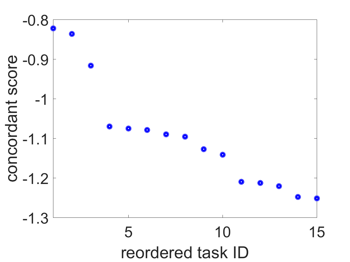
6.4.4 Detection of Anomaly Tasks
We set . The number of tasks (responses) . The information about the true s and numbers of different types of tasks is in Table 2. Other settings are the same as in Section 6.4.2. In Table 2, it can be seen that the true of the majority of tasks (the first 20 tasks) is 4. The first 20 tasks are referred to as concordant tasks, while the other 10 tasks are referred to as anomaly tasks.
| Group | True k | #Gaussian | #Bernoulli | #Poisson |
| 1 | 4 | 5 | 10 | 5 |
| 2 | 1 | 1 | 1 | 1 |
| 3 | 6 | 1 | 0 | 0 |
| 4 | 2 | 1 | 1 | 0 |
| 5 | 3 | 0 | 1 | 1 |
| 6 | 5 | 1 | 1 | 0 |
We compute the concordant scores using (15) for the tasks. In Fig 3, the concordant scores separate concordant tasks and anomaly tasks quite well. Scores of Poisson tasks are similar to scores of Bernoulli tasks, because they all provide less accurate information than Gaussian tasks do.


6.4.5 Handling Clustered Relationship among tasks
We construct 4 groups of tasks. The total number of tasks (responses) . The information about the true s and numbers of different types of tasks is in Table 3. Other settings are the same as in Section 6.4.4. We first apply Single for each task, setting . Then we apply the strategy in Section 4.3 to construct a similarity matrix by NMI defined in (16). Kernel PCA (Schölkopf et al, 1998; Van Der Maaten et al, 2009) is then applied using the similarity matrix as the kernel matrix. The similarity matrix and the result of Kernel PCA are shown in Fig 4.
| Group | True k | #Gaussian | #Bernoulli | #Poisson |
| 1 | 1 | 3 | 10 | 2 |
| 2 | 2 | 3 | 10 | 2 |
| 3 | 3 | 3 | 10 | 2 |
| 4 | 4 | 3 | 10 | 2 |


In Fig 4 (a), Group 2,3 and 4 can be recognized as three groups. In Group 1, each task shows no similarity with other tasks, because with the true , the data samples can be randomly partitioned into sub-populations, which results in low NMI scores. In Fig 4 (b), basically, 4 groups of tasks are clustered into 4 different regions.
6.4.6 Handling Outlier Samples
We choose the data set used in Section 6.4.2 with the true , then randomly shuffle the data pairs , for , and contaminate the true targets by the following procedure. For outlier ratio , (1) for Gaussian targets, set all the targets of of data samples to be ; (2) for Bernoulli targets, set all the targets of of data samples to be . Such contamination is only performed on training and validation data, leaving testing data clean.
Then we evaluate two groups of methods. For the group of non-robust methods, we choose our Hermit methods Mix and Mix GS. For the group of robust methods, we firstly run the robust version of the non-robust methods by adding in the natural parameter models as (11) and adding (13) as the additional penalty, then we clean the data by removing of data samples associated with the largest value of (). Finally, we run their non-robust version of methods on the “cleaned” data, respectively. We follow Gong et al (2012a) to adopt such two-stage strategy.
The imputation performances are reported in Table 4, from where it can be seen that, 1) when , robust methods are over-parameterized and may underperform non-robust methods; 2) when , robust methods significantly outperform non-robust methods.
| 0% | 1% | 2% | 5% | 8% | 10% | |||
|---|---|---|---|---|---|---|---|---|
| nMSE for Gaussian | Mix | non-robust | 0.0625 | 0.6754 | 0.6894 | 1.0122 | 1.3250 | 1.4953 |
| robust | 0.0620 | 0.0627 | 0.0626 | 0.0737 | 0.0632 | 0.0635 | ||
| Mix GS | non-robust | 0.0658 | 0.6434 | 0.6741 | 0.7505 | 1.0736 | 1.2939 | |
| robust | 0.0599 | 0.0611 | 0.0673 | 0.0694 | 0.0602 | 0.0607 | ||
| aAUC | Mix | non-robust | 0.9571 | 0.7954 | 0.7961 | 0.7982 | 0.7986 | 0.7981 |
| robust | 0.9570 | 0.9571 | 0.9574 | 0.9519 | 0.9568 | 0.9567 | ||
| Mix GS | non-robust | 0.9509 | 0.7979 | 0.7984 | 0.7982 | 0.7979 | 0.7952 | |
| robust | 0.9581 | 0.9577 | 0.9519 | 0.9482 | 0.9578 | 0.9574 | ||
| nMSE for Poisson | Mix | non-robust | 0.2089 | 0.7368 | 0.6905 | 0.6528 | 0.6642 | 0.6736 |
| robust | 0.2086 | 0.2105 | 0.2099 | 0.2345 | 0.2222 | 0.2230 | ||
| Mix GS | non-robust | 0.2136 | 0.7416 | 0.7795 | 0.6587 | 0.6688 | 0.8665 | |
| robust | 0.2087 | 0.2109 | 0.2169 | 0.2202 | 0.2212 | 0.2236 |
6.4.7 Feature-Based Prediction by MOE
We set the true . The true , whose first four rows are non-zero. The non-zero entries of are drawn from . Number of data samples . For all , the th data sample coming from the th sub-population obeys a multinomial distribution with the probability defined in (17). Other settings are the same as in Section 6.4.3.
We compare our Hermit methods Mix MOE and Mix MOE GS. The prediction performances are shown in Table 5, which are consistent with the results in Section 6.4.3.
We further show in Table 6 the concordance between and , where denotes the true , for all , for both training and testing data. In (22), is optimized by partially minimizing the discrepancy between and for . As such we also show the concordance between and . The concordances are measured by NMI defined in (16). We use NMI instead of KL-divergence, because NMI is normalized to the range of .
Both and are approximated accurately on the training data. The approximation accuracies are lower on the testing data because the deficiency of data samples comparing with the dimension.
| nMSE | aAUC | |
|---|---|---|
| LASSO | 0.6390 | 0.7834 |
| Mix MOE | 0.0656 | 0.9466 |
| Group LASSO | 0.6348 | 0.7878 |
| Mix MOE GS | 0.0579 | 0.9502 |
| Sep L2 | 0.6481 | 0.7794 |
| GO-MTL | 0.6946 | 0.7778 |
| CMTL | 0.6496 | 0.7796 |
| MSMTFL | 0.6397 | 0.7831 |
| TraceReg | 0.6509 | 0.7790 |
| SparseTrace | 0.6473 | 0.7805 |
| RMTL | 0.6511 | 0.7797 |
| Dirty | 0.6348 | 0.7878 |
| rMTFL | 0.6483 | 0.7787 |
| Training | Testing | |||
|---|---|---|---|---|
| Mix MOE | 0.9863 | 0.9918 | 0.8440 | 0.8457 |
| Mix MOE GS | 0.9962 | 0.9933 | 0.8455 | 0.8516 |
6.4.8 Scalability
We discuss the scalability of our method for increasing number of features and tasks. The running time is evaluated. We choose the data set used in Section 6.4.2 with the true . The sparsity is fixed to be 4. We set the number of features and the number of tasks . The ratios between the numbers of Gaussian, Bernoulli and Poisson tasks are the same as in Section 6.4.2. We randomly generate 100 data sets for each pair of . We report the results of the method Mix GS only, as the results of Mix are similar. In each case, is tuned and is equal to the true . The estimated parameters in different cases may have different numbers of relevant features. As such, in order to provide a fair comparison, we report the running time per feature, i.e., running time divided by the number of non-zero features of the estimated parameters in each case.
In Fig 5, both dimension and the number of tasks have no significant influence on running time per feature, especially when and is large, which is consistent with our time-complexity analysis in Section 3.2.


6.5 Application
On the real-world data sets, we first demonstrate the existence of the heterogeneity of conditional relationship, then report the superiority of our Hermit method over other methods considered in Section 6.1. We further interpret the advantage of our method by presenting the selected features. Effectiveness of anomaly-task detection and task clustering strategy is also validated.
6.5.1 Data Description
Both real-world data sets introduced in the following are longitudinal surveys for elder patients, which includes a set of questions. Some of the question answers are treated as input features and some of the questions related to indices of geriatric assessments are treated as targets.
LSOA II Data. This data is from the Second Longitudinal Study of Aging (LSOA II) 111https://www.cdc.gov/nchs/lsoa/lsoa2.htm.. LSOA II is a collaborative study by the National Center for Health Statistics (NCHS) and the National Institute of Aging conducted from 1994-2000. A national representative sample of subjects years of age and over were selected and interviewed. Three separated interviews were conducted during the periods of 1994-1996, 1997-1998, and 1999-2000, respectively. The interviews are referred to as WAVE 1, WAVE 2, and WAVE 3 interviews, respectively. We use data WAVE 2 and WAVE 3, which includes a total of sample subjects and 44 targets, and features are extracted from WAVE 2 interview.
Among the targets, specifically, three self-rated health measures, including overall health status, memory status and depression status, can be regarded as continuous outcomes; there are 41 binary outcomes, which fall into several categories: fundamental daily activity, extended daily activity, social involvement, medical condition, on cognitive ability, and sensation condition. The features include records of demographics, family structure, daily personal care, medical history, social activity, health opinion, behavior, nutrition, health insurance and income and assets, the majority of which are binary measurements. Both targets and features have missing values due to non-response and questionnaire filtering. The average missing value rates in targets and features are 13.7% and 20.2%, respectively. For the missing values in features, we adopt the following procedure for pre-processing. For continuous features, the missing values are imputed with sample mean. For binary features, a better approach is to treat missing as a third category as it may also carry important information; as such, two dummy variables are created from each binary feature with missing values (the third one is not necessary.) This results in totally features. We randomly select 30% of the samples for training, 30% for validation and the rest for testing.
easySHARE Data. This data is a simplified data set from the Survey of Heath, Aging, and Retirement in Europe (SHARE)222http://www.share-project.org/data-access-documentation.html.. SHARE includes multidisciplinary and cross-national panel databases on health, socio-economic status, and social and family networks of more than 85,000 individuals from European countries aged or over. Four waves of interviews were conducted during 2004 - 2011, and are referred to as WAVE 1 to WAVE 4 interviews. We use WAVE 1 and WAVE 2, which includes 20,449 sample persons and 15 targets (among which 11 are binary, and 4 are continuous), and totally 75 features are constructed from WAVE 1 interview.
The targets are from four interview modules: social support, mental health, functional limitation indices and cognitive function indices. The features cover a wide range of assessments, including demographics, household composition, social support and network, physical health, mental health, behavior risk, healthcare, occupation and income. Detailed description features are not listed in this paper. Both targets and features have missing values due to non-response and questionnaire filtering. The average missing value rates in targets and features are 6.9% and 5.1%, respectively. The same pre-processing procedure as that for LSOA II Data has been adopted and results in totally features. We randomly select 10% of the samples for training, 10% for validation and the rest for testing.
6.5.2 Comparison with FMR Method
In this experiment, we compare our proposed Hermit methods Mix and Mix GS which handle mixed type of outcomes with Sep which learns different types of tasks separately. Single is abandoned because it learns each task independently and is not able to use targets of other tasks to help increasing imputation performance.
Results are reported in Fig 6, where 1) for both the real data sets, basically, the best pre-fixed , except for Bernoulli tasks of easySHARE data, suggesting that the heterogeneity of conditional relationship exists in LSOA II data and the Gaussian tasks of easySHARE data; 2) FMR models benefit Gaussian targets more than Bernoulli targets; 3) Mix and Mix GS outperform Sep in Gaussian tasks. However, their performances are comparable with Sep in Bernoulli tasks, which may be because that the number of Bernoulli tasks are much more than that of Gaussian tasks such that the benefit from Gaussian tasks is limited.


6.5.3 Comparison with Non-FMR Methods
In this experiment we test imputation performance, comparing our Hermit methods Mix and Mix GS with all the non-FMR methods.
Results are reported in Table 7, where 1) our Hermit methods Mix and Mix GS not only outperform their special cases, LASSO and Group LASSO, respectively, but also outperform other methods, including those handling certain kinds of heterogeneities, except for aAUC on easySHARE, the reason of which has been discussed in Section 6.5.2; 2) Mix GS increases nMSE by 9.76% and 14.37% on LSOA II data and easySHARE data, respectively, comparing with its non-FMR version Group LASSO. The similar improvements by Mix are witnessed as well.
| LSOA II | easySHARE | |||
|---|---|---|---|---|
| nMSE | aAUC | nMSE | aAUC | |
| LASSO | 0.7051 | 0.7474 | 0.7869 | 0.7386 |
| Mix | 0.6408 | 0.7525 | 0.6601 | 0.7419 |
| Group LASSO | 0.6975 | 0.7413 | 0.7897 | 0.7413 |
| Mix GS | 0.6294 | 0.7481 | 0.6548 | 0.7402 |
| Sep L2 | 0.7176 | 0.7392 | 0.7796 | 0.7464 |
| GO-MTL | 0.8516 | 0.6972 | 0.8231 | 0.7288 |
| CMTL | 0.8186 | 0.7089 | 0.7958 | 0.7364 |
| MSMTFL | 0.7028 | 0.7473 | 0.7803 | 0.7411 |
| TraceReg | 0.7150 | 0.7408 | 0.7809 | 0.7496 |
| SparseTrace | 0.6972 | 0.7475 | 0.7791 | 0.7475 |
| RMTL | 0.7145 | 0.7418 | 0.7808 | 0.7496 |
| Dirty | 0.7032 | 0.7480 | 0.7781 | 0.7486 |
| rMTFL | 0.6953 | 0.7418 | 0.7781 | 0.7486 |
6.5.4 Feature Selection
We consider demonstrating the advantage of our Hermit method on feature selection. We compare our Hermit method Mix GS with its non-FMR version Group LASSO. Both methods select shared features across tasks. We collect the unique features that only selected for each sub-population.
For LSOA II data set, the tuned . Mix GS selects features (summing up selected features of both sub-populations), while Group LASSO selects features. Descriptions of unique features of both sub-populations are listed in Table 8. Sub-population 1 seems considering worse condition of patients.
| Sub-population 1 () | Sub-population 2 () |
|---|---|
| able or prevented to leave house | times seen doctor in past 3 months |
| have problems with balance | easier or harder to walk 1/4 mile |
| total number of living children | widowed |
| easier/harder than before: in/out of bed | follow regular physical routine |
| #(ADL activities) SP is unable to perform | present social activities |
| easier or harder to walk 10 steps | ever had a stress test |
| do you take aspirin | do you take vitamins |
| often troubled with pain | necessary to use steps or stairs |
| visit homebound friend for others | had flu shot |
| ever had a hysterectomy | ever had cataract surgery |
| physical activity more/less/same |
For easySHARE data set, the tuned . Mix GS selects features, while Group LASSO selects features. Descriptions of unique features of two sub-populations are listed in Table 9. Sub-population 1 seems considering more about personality and experience, while sub-population 2 seems considering more about politics and education.
For both real data sets, our Hermit method Mix GS recalls more useful features than Group LASSO does.
| Sub-population 1 () | Sub-population 2 () |
|---|---|
| fatigue | taken part in a political organization |
| guilt | attended an educational or training course |
| enjoyment | taken part in religious organization |
| suicidality | none of social activities |
| tearfullness | cared for a sick or disabled adult |
| interest | done voluntary or charity work |
| current job situation:sick | education: lower secondary |
| education: first tertiary | |
| education: post secondary | |
| education: upper secondary | |
| education: primary | |
| education: second tertiary |
6.5.5 Detection of Anomaly Tasks
We firstly use (15) to compute concordant scores of tasks, which are reported in Fig 7. Clear separations are witnessed on both data sets. We select one-third of tasks with highest scores as concordant tasks and another third with lowest scores as anomaly tasks. The descriptions of the concordant and anomaly tasks are listed in Table 10 and Table 11, respectively.

| Concordant tasks (top 7) | Anomaly tasks (top 8) |
|---|---|
| have difficulty dressing | go to movies, sports, events, etc. |
| have difficulty doing light housewrk | now have asthma |
| have difficulty using toilet | now have arthritis |
| have difficulty managing medication | now have hypertension |
| have difficulty bathing or showering | injured from fall(s) |
| have difficulty managing money | memory of year |
| have difficulty preparing meals | have deafness |
| get together with relatives |
| Concordant tasks (top 5) | Anomaly tasks (top 5) |
|---|---|
| activities of daily living index | numeracy score |
| instrumental activities of daily living indices | gone to sport social or other kind of club |
| mobility index | recall of words first trial |
| appetite | give help to others outside the household |
| orientation to date | provided help to family friends or neighbors |
The concordant tasks detected by our methods seem truly correlated with each other intuitively. And the information of detected anomaly tasks is diverse and seems different with that of concordant tasks.
For each data set, we apply our Hermit method Mix (and Mix GS) to build two models for non-anomaly tasks (the first two-third tasks) and anomaly tasks, respectively. For LSOA II data set, the tuned and for non-anomaly tasks and anomaly tasks, respectively. For easySHARE data set, the tuned and for non-anomaly tasks and anomaly tasks, respectively.
Averaged imputation performances are shown in Table 12. By providing separate models to handle anomaly tasks, the performances improve significantly, where Mix GS outperforms Mix, maybe because the non-anomaly tasks share some relevant features.
| LSOA II | easySHARE | |||
|---|---|---|---|---|
| nMSE | aAUC | nMSE | aAUC | |
| Mix - All tasks | 0.6408 | 0.7525 | 0.6601 | 0.7419 |
| Mix - Handle anomalies | 0.5979 | 0.7602 | 0.6569 | 0.7370 |
| Mix GS - All tasks | 0.6294 | 0.7481 | 0.6548 | 0.7402 |
| Mix GS - Handle anomalies | 0.5923 | 0.7649 | 0.6462 | 0.7447 |
6.5.6 Handling Clustered Relationship among tasks
We adopt the same strategy as that in Section 6.4.5 to construct a similarity matrix and perform dimension reduction for each of the real-world data sets.
For LSOA II data set, the similarity matrix and results of 2D reduction are shown in Fig 8. In Fig 8(b), tasks are partitioned into groups. We apply k-means algorithm to separate the tasks into 4 groups. Tasks in Group 1 are mainly about current status. The descriptions of tasks of Group 2 are “how often felt sad or depressed in the past 12 months” and “self rated memory”. Tasks in Group 3 and 4 are about having difficulty performing some certain actions. Group 3 is similar to Group 4, which can be reflected by Fig 8(b).


For easySHARE data set, the similarity matrix and results of 2D reduction are shown in Fig 9. In Fig 9(b), tasks are partitioned into groups as well. We also apply k-means algorithm to separate the tasks into 4 groups. The descriptions of tasks for each group are shown in Table 13, where descriptions of 4 types of interview modules are basically separated into 4 groups, respectively. The only “misclassified” task with the description of “Orientation to date” seems to be more related to other tasks in Group 2 than the tasks in Group 4.


| Group | Targets | Interview module |
|---|---|---|
| 1 | Activities of daily living index | Functional Limitation Indices |
| Instrumental activities of daily living index | Functional Limitation Indices | |
| Mobility index | Functional Limitation Indices | |
| 2 | Depression | Mental Health |
| Pessimism | Mental Health | |
| Sleep | Mental Health | |
| Irritability | Mental Health | |
| Appetite | Mental Health | |
| Concentration | Mental Health | |
| Orientation to date | Cognitive Function Indices | |
| 3 | Provided help to family friends or neighbors | Social Support & Network |
| Gone to sport social or other kind of club | Social Support & Network | |
| Give help to others outside the household | Social Support & Network | |
| 4 | Recall of words score | Cognitive Function Indices |
| Numeracy score | Cognitive Function Indices |
For each data set, we further apply our Hermit methods Mix and Mix GS for each group of tasks. For LSOA II data set, tuned and for Group 1,2,3 and 4, respectively. For easySHARE data set, tuned and for Group 1,2,3 and 4, respectively. Imputation performances are shown in Table 14. Performances increase by building separate models for each group, suggesting that separate models for clustered tasks are more accurate.
| LSOA II | easySHARE | |||
|---|---|---|---|---|
| nMSE | aAUC | nMSE | aAUC | |
| Mix - All tasks | 0.6408 | 0.7525 | 0.6601 | 0.7419 |
| Mix - Clustered tasks | 0.6370 | 0.7592 | 0.6552 | 0.7439 |
| Mix GS - All tasks | 0.6294 | 0.7481 | 0.6548 | 0.7402 |
| Mix GS - Clustered tasks | 0.6202 | 0.7559 | 0.6533 | 0.7474 |
6.5.7 Feature-Based Prediction by MOE
We compare the methods using only features to predict targets on both real-world data sets. Our proposed MOE type of Hermit methods, Mix MOE and Mix MOE GS, are compared with the non-FMR methods. We also integrate our strategies to handle anomaly tasks and clustered structure among tasks in both our proposed MOE type of Hermit methods Mix MOE and Mix MOE GS. Concretely, we use the anomaly-task detection results in Section 6.5.5 and the task clustering results in Section 6.5.6.
The prediction results are reported in Table 15. Our proposed Hermit method Mix MOE and Mix MOE GS outperform baseline methods on LSOA II and on Gaussian tasks of easySHARE, which is consistent with the results in Table 7. In addition, by integrating our task clustering strategy, our proposed Hermit methods Mix MOE TC and Mix MOE GS TC outperform other methods on Gaussian targets, while providing comparable results on Bernoulli tasks. Mix MOE TC and Mix MOE GS TC even outperform our proposed Hermit methods Mix MOE Robust and Mix MOE GS Robust on Gaussian targets, suggesting that it is more accurate to build a specific model for each cluster of tasks.
Comparing Table 15 with Table 7, our MOE methods do not rival our FMR methods. We investigate the reason by showing the concordance between and ( is defined in equation 21) in Table 16. In Table 16, the concordances of conditional probabilities measured by NMI are generally low, especially comparing with the results in Table 6, suggesting that on both real-world data sets, it is difficult to learn the mixture probabilities.
| LSOA II | easySHARE | |||
| nMSE | aAUC | nMSE | aAUC | |
| LASSO | 0.7051 | 0.7474 | 0.7869 | 0.7386 |
| Group LASSO | 0.6975 | 0.7413 | 0.7897 | 0.7413 |
| MSMTFL | 0.7028 | 0.7473 | 0.7803 | 0.7411 |
| Sep L2 | 0.7176 | 0.7392 | 0.7796 | 0.7464 |
| GO-MTL | 0.8516 | 0.6972 | 0.8231 | 0.7288 |
| CMTL | 0.8186 | 0.7089 | 0.7958 | 0.7364 |
| TraceReg | 0.7150 | 0.7408 | 0.7809 | 0.7496 |
| SparseTrace | 0.6972 | 0.7475 | 0.7791 | 0.7475 |
| RMTL | 0.7145 | 0.7418 | 0.7808 | 0.7496 |
| Dirty | 0.7032 | 0.7480 | 0.7781 | 0.7486 |
| rMTFL | 0.6953 | 0.7418 | 0.7781 | 0.7486 |
| Mix MOE | 0.6935 | 0.7504 | 0.7991 | 0.7395 |
| Mix MOE GS | 0.7054 | 0.7438 | 0.7774 | 0.7387 |
| Mix MOE Robust | 0.6906 | 0.7436 | 0.7642 | 0.7351 |
| Mix MOE GS Robust | 0.6981 | 0.7430 | 0.7668 | 0.7344 |
| Mix MOE TC | 0.6859 | 0.7333 | 0.7584 | 0.7389 |
| Mix MOE GS TC | 0.6925 | 0.7379 | 0.7657 | 0.7367 |
| LSOA II | easySHARE | |||
|---|---|---|---|---|
| Training | Testing | Training | Testing | |
| Mix MOE | 0.2745 | 0.1301 | 0.1314 | 0.1068 |
| Mix MOE GS | 0.1060 | 0.0673 | 0.2527 | 0.2054 |
7 Discussions & Conclusions
In this paper, we propose a novel model Hermit to explore heterogeneities of conditional relationship, output type and shared information among tasks. Based on multivariate-target FMR and MOE models, our model jointly learns tasks with mixed type of output, allows incomplete data in the output, imposes inner component-wise group constraint and handles anomaly tasks and clustered structure among tasks. These key elements are integrated in a unified generalized mixture model setup so that they can benefit from and reinforce each other to discover the triple heterogeneities in data. Rigorous theoretical analyses under the high dimensional framework are provided.
We mainly consider the special setting of MTL, where the multivariate outcomes share the same set of instances and the same set of features because our main objective is to learn potentially shared sample clusters and feature sets among tasks. However, as stressed in the introduction, the main definition of MTL considers tasks that do not necessarily share the same set of samples/instances and the same set of features, such as distributed learning systems (different tasks have entirely different data instances, see Jin et al 2006 and Boyd et al 2011) and multi-source learning systems (different tasks have entirely different feature spaces, see Zhang and Yeung 2011 and Jin et al 2015). For such cases, one can define the specific expected shared information among tasks and then extend our methodology. For example, although tasks do not share the same instances, they could share the same mixture model structure. Then for the distributed learning systems, our model in Section 3 can still be applied. Additionally, the tasks could still share the pattern/sparsity in feature selection even though the feature sets are different, e.g., Liu et al (2009) and Gong et al (2012b). Then one can build FMR models for the tasks in which the regression coefficient vectors of the tasks share the same sparsity pattern achieved by group penalization. The case of multi-source learning systems can also be handled similarly by embedding features into a shared feature space, e.g., Zhang and Yeung (2011) and Jin et al (2015).
There are many interesting future directions. It is worthwhile to explore the theoretical and empirical performance of non-convex penalties. Meanwhile, different components should share some features, and overlapping cluster pattern of conditional relationship should also be considered in real applications, both of which require further investigation. It is also interesting to explore other low-dimensional structures in the natural parameters, e.g., low-rank structure and its sparse composition (Chen et al, 2012b). Our strategies on handling anomaly tasks and clustered structure among tasks require two stages. It is worthwhile to explore one-stage models to handle such task heterogeneities during a whole learning process. More complicated structure among tasks, such as graph-based structure, should also be explored. Our theoretical results cover our method introduced in Section 3 and robust estimation introduced in Section 4.1. Nonetheless, theoretical guarantees for other extensions in Section 4 are still challenging due to joint learning complicated relationship among tasks and population heterogeneity, which will be focused on in our future research.
Acknowledgements.
The authors would like to thank the editors and reviewers for their valuable suggestions on improving this paper. This work of Jian Liang and Changshui Zhang is (jointly or partly) funded by National Natural Science Foundation of China under Grant No.61473167 and Beijing Natural Science Foundation under Grant No. L172037. Kun Chen’s work is partially supported by U.S. National Science Foundation under Grants DMS-1613295 and IIS-1718798. The work of Fei Wang is supported by National Science Foundation under Grants IIS-1650723 and IIS-1716432.Appendix A Definitions
Definition 1
has a sub-exponential distribution with parameters if for , it holds
Appendix B The Empirical Process
In order to prove the first part of Theorem 1 that the bound in (26) has the probability in (25), we firstly follow Städler et al (2010) to define the empirical process for fixed data points . For and , let
By fixing some and , we define an event below, upon which the bound in (26) can be proved. So the probability of the event is the probability in (25).
| (21) |
It can be seen that, (21) defines a set of the parameter , and the bound in (26) will be proved with in the set.
For group-lasso type estimator, define an event similar to that in (21) in the following.
| (22) |
Appendix C Lemmas
In order to show that the probability of event is large, we firstly invoke the following lemma.
Lemma 2
A proof is given in Appendix F.
Then we can follow the Corollary 1 in Städler et al (2010) to show that the probability of event is large below.
Lemma 3
A proof is given in Appendix G.
Appendix D Corollaries for Models Considering Outlier Samples
When considering outlier samples and modifying the natural parameter model as in (11), we can show in this section the similar results.
First, as and are treated in the similar way, we denote them together by , and such that for all ,
where is a identity matrix.
Thus it can be seen that the modification only results in new design matrix and regression coefficient matrix, therefore, we can apply Theorem 1 3 to have similar results for the modified models.
For lasso-type penalties, denote the set of indices of non-zero entries of by , and the set of indices of non-zero entries of by , where . Denote by . Then for entry-wise penalties in (5) (for ) with and (for ), we need the following modified restricted eigenvalue condition.
Condition 6
For all and all satisfying , it holds for some constant that,
Corollary 1
Consider the Hermit model in (1) with , and consider the penalized estimator (12) with the penalties in (5) and .
(a) Assume conditions 1-3 and 6 hold. Suppose , and take for some constant . For some constant and large enough , with probability we have
(b) Assume conditions 1-3 hold (without condition 6), assume
as . If for some sufficiently large, and for some constant and large enough , with the following probability we have
For group-lasso type penalties, denote
where and denote the th group of and the th group of , respectively. Now denote with some abuse of notation.
Then for group penalties in (27) (for ) and (for ), we need the following modified restricted eigenvalue condition.
Condition 7
For all and all satisfying
it holds that for some constant ,
Corollary 2
Consider the Hermit model in (1) with , and consider estimator (12) with the group penalties in (27) and .
(a) Assume conditions 1-3 and 7 hold. Suppose , and take for some constant . For some constant and large enough , with probability we have
(b) Assume conditions 1-3 hold (without condition 7), assume
as . If for some sufficiently large, and for some constant and large enough , with the following probability we have
Appendix E Proof of Lemma 1
Proof
For non-negative continuous variable , we have
Similarly, we have
For sub-exponential with parameters such that for
we have the following.
If , we have
and similarly,
If , we have and .
Then for some constants , for non-negative continuous variable which is sub-exponential with parameters , for and , we have
If , . And if , . And .
For non-negative discrete variables, the result is the same.
The result of Lemma 1 follows from the result above, has a finite mixture distribution for and the following.
When dispersion parameter is known, for a constant depending on , we have
Appendix F Proof of Lemma 2
Appendix G Proof of Lemma 3
Proof
We use the following norm introduced in the Proof of Lemma 2 in Städler et al (2010) and use as the entropy of covering number (see Van de Geer (2000)) which is equipped the metric induced by the norm for a collection of functions on ,
Define .
Lemma 4
(Entropy Lemma) For a constant , for all and , we have
Proof
(For Entropy Lemma) The difference between this proof and that of Entropy Lemma in the proof of Lemma 2 of Städler et al (2010) is in the notations and the effect of multivariate responses.
For multivariate responses we have for ,
where is the maximum of dimension of for .
Under the definition of the norm we have
Then by the result of Städler et al (2010) we have
where is the dimension of .
And we follow Städler et al (2010) to apply Lemma 2.6.11 of Van Der Vaart and Wellner (1996) to give a bound as
Thus we can get
Now we turn to prove Lemma 3.
We follow Städler et al (2010) to use the truncated version of the empirical process below.
We follow Städler et al (2010) to apply the Lemma 3.2 in Van de Geer (2000) and a conditional version of Lemma 3.3 in Van de Geer (2000) to the class
For some constants depending on and in Condition 2 of Städler et al (2010), using the notation of Lemma 3.2 in Van de Geer (2000), we follow Städler et al (2010) to choose and .
Thus we by choosing we can satisfy the condition of Lemma 3.2 of Van de Geer (2000) to have
Now for the rest we can apply Lemma 3.2 of Van de Geer (2000) to give the same result with Lemma 2 of Städler et al (2010).
So we have
with probability at least
At last, for the case when , for , we have
and
Then the probability of the following inequality under our model is given in Lemma 2.
where .
Appendix H Proof of Theorem 1
Proof
This proof mostly follows that of Theorem 3 of Städler et al (2010). The only difference is in the notations. As such, we omit the details.
Appendix I Proof of Theorem 2
Proof
This proof also mostly follows that of Theorem 5 of Städler et al (2010). The difference is in the notations and the choice of .
If the event happens, with for some constants , where depends on ,
we have
Under the definition of in (23) we have . And as we have for sufficiently large.
As sufficiently large we have .
And using the condition on and , we have both and , so we have .
At last, as the event has large probability, we have
Appendix J Proof of Theorem 3
Proof
First we discuss the bound for the probability of in (22).
The difference between and in (21) is only related to the following entropy of the Entropy Lemma in the proof of Lemma 3.
where still maintains a convex hull for in the metric space equipped with the metric induced by the norm defined in the proof of Lemma 3. Thus it still satisfies the condition of Lemma 2.6.11 of Van Der Vaart and Wellner (1996) which can still be applied to give
So the probability of event remains the same form with that in Lemma 3.
Then we discuss the bound for the average excess risk and feature selection.
Case 1 When the following is true:
we have
Case 2 When the following is true:
As , we have
Then we get
Case 3 When the following is true:
we have
Thus we have
so we can use the Condition 5 for to have
So we have
References
- Aho et al (2014) Aho K, Derryberry D, Peterson T (2014) Model selection for ecologists: the worldviews of AIC and BIC. Ecology 95(3):631–636
- Alfò et al (2016) Alfò M, Salvati N, Ranallli MG (2016) Finite mixtures of quantile and M-quantile regression models. Statistics and Computing pp 1–24
- Argyriou et al (2007a) Argyriou A, Evgeniou T, Pontil M (2007a) Multi-task feature learning. In: Advances in Neural Information Processing Systems, pp 41–48
- Argyriou et al (2007b) Argyriou A, Pontil M, Ying Y, Micchelli CA (2007b) A spectral regularization framework for multi-task structure learning. In: Advances in Neural Information Processing Systems, pp 25–32
- Bai et al (2016) Bai X, Chen K, Yao W (2016) Mixture of linear mixed models using multivariate t distribution. Journal of Statistical Computation and Simulation 86(4):771–787
- Bartolucci and Scaccia (2005) Bartolucci F, Scaccia L (2005) The use of mixtures for dealing with non-normal regression errors. Computational Statistics & Data Analysis 48(4):821–834
- Barzilai and Borwein (1988) Barzilai J, Borwein JM (1988) Two-point step size gradient methods. IMA Journal of Numerical Analysis 8(1):141–148
- Becker et al (2011) Becker SR, Candès EJ, Grant MC (2011) Templates for convex cone problems with applications to sparse signal recovery. Mathematical Programming Computation 3(3):165–218
- Bhat and Kumar (2010) Bhat HS, Kumar N (2010) On the derivation of the Bayesian Information Criterion. School of Natural Sciences, University of California
- Bickel et al (2009) Bickel PJ, Ritov Y, Tsybakov AB (2009) Simultaneous analysis of Lasso and Dantzig selector. The Annals of Statistics pp 1705–1732
- Bishop (2006) Bishop CM (2006) Pattern recognition. Machine Learning 128:1–58
- Boyd et al (2011) Boyd S, Parikh N, Chu E, Peleato B, Eckstein J (2011) Distributed optimization and statistical learning via the alternating direction method of multipliers. Foundations and Trends® in Machine Learning 3(1):1–122
- Candès and Recht (2009) Candès EJ, Recht B (2009) Exact matrix completion via convex optimization. Found Comput Math 9(6):717–772
- Chen et al (2011) Chen J, Zhou J, Ye J (2011) Integrating low-rank and group-sparse structures for robust multi-task learning. In: Proceedings of the 17th ACM SIGKDD International Conference on Knowledge Discovery and Data Mining, ACM, pp 42–50
- Chen et al (2012a) Chen J, Liu J, Ye J (2012a) Learning incoherent sparse and low-rank patterns from multiple tasks. ACM Transactions on Knowledge Discovery from Data (TKDD) 5(4):22
- Chen et al (2012b) Chen K, Chan KS, Stenseth NC (2012b) Reduced rank stochastic regression with a sparse singular value decomposition. Journal of the Royal Statistical Society: Series B (Statistical Methodology) 74(2):203–221
- Chen et al (2010) Chen X, Kim S, Lin Q, Carbonell JG, Xing EP (2010) Graph-structured multi-task regression and an efficient optimization method for general fused lasso. arXiv preprint arXiv:10053579
- Cover and Thomas (2012) Cover TM, Thomas JA (2012) Elements of information theory. John Wiley & Sons
- Dempster et al (1977) Dempster AP, Laird NM, Rubin DB (1977) Maximum likelihood from incomplete data via the EM algorithm. Journal of the Royal Statistical Society Series B (methodological) pp 1–38
- Doğru and Arslan (2016) Doğru FZ, Arslan O (2016) Robust mixture regression using mixture of different distributions. In: Recent Advances in Robust Statistics: Theory and Applications, Springer, pp 57–79
- Do˘ru and Arslan (2017) Do˘ru FZ, Arslan O (2017) Parameter estimation for mixtures of skew Laplace normal distributions and application in mixture regression modeling. Communications in Statistics-Theory and Methods 46(21):10,879–10,896
- Fahrmeir et al (2013) Fahrmeir L, Kneib T, Lang S, Marx B (2013) Regression: models, methods and applications. Springer Science & Business Media
- Fan and Lv (2010) Fan J, Lv J (2010) A selective overview of variable selection in high dimensional feature space. Statistica Sinica 20(1):101–148
- Fern and Brodley (2003) Fern XZ, Brodley CE (2003) Random projection for high dimensional data clustering: A cluster ensemble approach. In: Proceedings of the 20th International Conference on Machine Learning (ICML-03), pp 186–193
- Van de Geer (2000) Van de Geer SA (2000) Applications of empirical process theory, vol 91. Cambridge University Press Cambridge
- Gong et al (2012a) Gong P, Ye J, Zhang C (2012a) Robust multi-task feature learning. In: Proceedings of the 18th ACM SIGKDD International Conference on Knowledge Discovery and Data Mining, ACM, pp 895–903
- Gong et al (2012b) Gong P, Ye J, Zhang Cs (2012b) Multi-stage multi-task feature learning. In: Advances in Neural Information Processing Systems, pp 1988–1996
- Hanley and McNeil (1982) Hanley JA, McNeil BJ (1982) The meaning and use of the area under a receiver operating characteristic (ROC) curve. Radiology 143(1):29–36
- He and Lawrence (2011) He J, Lawrence R (2011) A graph-based framework for multi-task multi-view learning. In: Proceedings of the 28th International Conference on Machine Learning (ICML-11), pp 25–32
- Huang et al (2012) Huang J, Breheny P, Ma S (2012) A selective review of group selection in high-dimensional models. Statistical Science 27(4):481–499
- Jacob et al (2009) Jacob L, Vert Jp, Bach FR (2009) Clustered multi-task learning: A convex formulation. In: Advances in Neural Information Processing Systems, pp 745–752
- Jacobs et al (1991) Jacobs RA, Jordan MI, Nowlan SJ, Hinton GE (1991) Adaptive mixtures of local experts. Neural Computation 3(1):79–87
- Jalali et al (2010) Jalali A, Sanghavi S, Ruan C, Ravikumar PK (2010) A dirty model for multi-task learning. In: Advances in Neural Information Processing Systems, pp 964–972
- Ji and Ye (2009) Ji S, Ye J (2009) An accelerated gradient method for trace norm minimization. In: Proceedings of the 26th Annual International Conference on Machine Learning, ACM, pp 457–464
- Jin et al (2006) Jin R, Goswami A, Agrawal G (2006) Fast and exact out-of-core and distributed k-means clustering. Knowledge and Information Systems 10(1):17–40
- Jin et al (2015) Jin X, Zhuang F, Pan SJ, Du C, Luo P, He Q (2015) Heterogeneous multi-task semantic feature learning for classification. In: Proceedings of the 24th ACM International on Conference on Information and Knowledge Management, ACM, pp 1847–1850
- Jorgensen (1987) Jorgensen B (1987) Exponential dispersion models. Journal of the Royal Statistical Society Series B (Methodological) pp 127–162
- Khalili (2011) Khalili A (2011) An overview of the new feature selection methods in finite mixture of regression models. Journal of Iranian Statistical Society 10(2):201–235
- Khalili and Chen (2007) Khalili A, Chen J (2007) Variable selection in finite mixture of regression models. Journal of the American Statistical Association 102(479):1025–1038
- Koller and Sahami (1996) Koller D, Sahami M (1996) Toward optimal feature selection
- Kubat (2015) Kubat M (2015) An introduction to machine learning. Springer
- Kumar and Daumé III (2012) Kumar A, Daumé III H (2012) Learning task grouping and overlap in multi-task learning. In: Proceedings of the 29th International Conference on Machine Learning, Omnipress, pp 1723–1730
- Kyung Lim et al (2016) Kyung Lim H, Narisetty NN, Cheon S (2016) Robust multivariate mixture regression models with incomplete data. Journal of Statistical Computation and Simulation pp 1–20
- Law et al (2002) Law MH, Jain AK, Figueiredo M (2002) Feature selection in mixture-based clustering. In: Advances in Neural Information Processing Systems, pp 625–632
- Li et al (2014) Li S, Liu ZQ, Chan AB (2014) Heterogeneous multi-task learning for human pose estimation with deep convolutional neural network. In: Proceedings of the IEEE Conference on Computer Vision and Pattern Recognition Workshops, pp 482–489
- Liu et al (2009) Liu J, Ji S, Ye J (2009) Multi-task feature learning via efficient -norm minimization. In: Proceedings of the 25th Conference on Uncertainty in Artificial Intelligence, AUAI Press, pp 339–348
- McLachlan and Peel (2004) McLachlan G, Peel D (2004) Finite mixture models. John Wiley & Sons
- Neal and Hinton (1998) Neal RM, Hinton GE (1998) A view of the EM algorithm that justifies incremental, sparse, and other variants. In: Learning in Graphical Models, Springer, pp 355–368
- Nelder and Baker (1972) Nelder JA, Baker RJ (1972) Generalized linear models. Encyclopedia of Statistical Sciences
- Nesterov et al (2007) Nesterov Y, et al (2007) Gradient methods for minimizing composite objective function. Tech. rep., UCL
- Passos et al (2012) Passos A, Rai P, Wainer J, Daumé III H (2012) Flexible modeling of latent task structures in multitask learning. In: Proceedings of the 29th International Conference on Machine Learning, Omnipress, pp 1283–1290
- Schölkopf et al (1998) Schölkopf B, Smola A, Müller KR (1998) Nonlinear component analysis as a kernel eigenvalue problem. Neural Computation 10(5):1299–1319
- She and Chen (2017) She Y, Chen K (2017) Robust reduced-rank regression. Biometrika 104(3):633–647
- She and Owen (2011) She Y, Owen AB (2011) Outlier detection using nonconvex penalized regression. Journal of the American Statistical Association 106(494):626–639
- Städler et al (2010) Städler N, Bühlmann P, Van De Geer S (2010) -penalization for mixture regression models. Test 19(2):209–256
- Strehl and Ghosh (2002a) Strehl A, Ghosh J (2002a) Cluster ensembles—a knowledge reuse framework for combining multiple partitions. Journal of Machine Learning Research 3(Dec):583–617
- Strehl and Ghosh (2002b) Strehl A, Ghosh J (2002b) Cluster ensembles: a knowledge reuse framework for combining partitionings. In: 18th National Conference on Artificial Intelligence, American Association for Artificial Intelligence, pp 93–98
- Tan et al (2010) Tan Z, Kaddoum R, Le Yi Wang HW (2010) Decision-oriented multi-outcome modeling for anesthesia patients. The Open Biomedical Engineering Journal 4:113
- Van Der Maaten et al (2009) Van Der Maaten L, Postma E, Van den Herik J (2009) Dimensionality reduction: A comparative. J Mach Learn Res 10:66–71
- Van Der Vaart and Wellner (1996) Van Der Vaart AW, Wellner JA (1996) Weak convergence. Springer
- Wedel and DeSarbo (1995) Wedel M, DeSarbo WS (1995) A mixture likelihood approach for generalized linear models. Journal of Classification 12(1):21–55
- Weruaga and Vía (2015) Weruaga L, Vía J (2015) Sparse multivariate gaussian mixture regression. IEEE Transactions on Neural Networks and Learning Systems 26(5):1098–1108
- Xian Wang et al (2004) Xian Wang H, bing Zhang Q, Luo B, Wei S (2004) Robust mixture modelling using multivariate t-distribution with missing information. Pattern Recognition Letters 25(6):701–710
- Yang et al (2009) Yang X, Kim S, Xing EP (2009) Heterogeneous multitask learning with joint sparsity constraints. In: Advances in Neural Information Processing Systems, pp 2151–2159
- Yuksel et al (2012) Yuksel SE, Wilson JN, Gader PD (2012) Twenty years of mixture of experts. IEEE Transactions on Neural Networks and Learning Systems 23(8):1177–1193
- Zhang et al (2012) Zhang D, Shen D, Initiative ADN, et al (2012) Multi-modal multi-task learning for joint prediction of multiple regression and classification variables in alzheimer’s disease. NeuroImage 59(2):895–907
- Zhang and Yeung (2011) Zhang Y, Yeung DY (2011) Multi-task learning in heterogeneous feature spaces. In: 25th AAAI Conference on Artificial Intelligence and the 23rd Innovative Applications of Artificial Intelligence Conference, AAAI-11/IAAI-11, San Francisco, CA, United States, 7-11 August 2011, Code 87049, Proceedings of the National Conference on Artificial Intelligence, p 574
- Zhou et al (2011) Zhou J, Chen J, Ye J (2011) Clustered multi-task learning via alternating structure optimization. In: Advances in Neural Information Processing Systems, pp 702–710