\copyyear

2023 \startpage1

\authormark

CARABALLO et al. \titlemarkBiot–Brinkman equations in vorticity form

\corres

Corresponding author Ricardo Ruiz-Baier.

\fundingInfo

Chilean Research and Technology Council through the ANID program for international research visits; by the Australian Government through the National Computational Infrastructure (NCI) under the ANU Merit Allocation Scheme (ANUMAS); and by the Australian Research Council through the Future Fellowship grant FT220100496 and Discovery Project grant DP22010316.

Robust finite element methods and solvers for the Biot–Brinkman equations in vorticity form

Ruben Caraballo Chansophea Wathanak In Alberto F. Martín Ricardo Ruiz-Baier \orgdivGIMNAP, Departamento de Matemática, \orgnameUniversidad del Bío-Bío, \orgaddress\stateConcepción, \countryChile \orgdivSchool of Mathematics, \orgnameMonash University, \orgaddress\state9 Rainforest Walk, Melbourne VIC 3800, \countryAustralia \orgdivSchool of Computing, \orgnameAustralian National University, \orgaddress\stateActon ACT 2601, \countryAustralia \orgnameUniversidad Adventista de Chile, \orgaddress\stateCasilla 7-D, Chillán, \countryChile [email protected] Caraballo R In CW Martín AF Ruiz-Baier R

(Date Month Year; Date Month Year)

Abstract

[Abstract]In this paper, we propose a new formulation and a suitable finite element method for the steady coupling of viscous flow in deformable porous media using divergence-conforming filtration fluxes. The proposed method is based on the use of parameter-weighted spaces, which allows for a more accurate and robust analysis of the continuous and discrete problems. Furthermore, we conduct a solvability analysis of the proposed method and derive optimal error estimates in appropriate norms. These error estimates are shown to be robust in a variety of regimes, including the case of large Lamé parameters and small permeability and storativity coefficients. To illustrate the effectiveness of the proposed method, we provide a few representative numerical examples, including convergence verification and testing of robustness of block-diagonal preconditioners with respect to model parameters.

\jnlcitation\cname

, , , and . \ctitleRobust finite element methods and solvers for the Biot–Brinkman equations in vorticity form. \cjournalNumer Methods PDEs. \cvol2023;00(00):1–18.

keywords:

Biot–Brinkman coupled problem, deformable porous media, vorticity-based formulation, mixed finite element methods.
Mathematics Subject Classifications (2000): 65N30, 65N15, 76S05, 35Q74.

^†^†articletype: Article Type^†^†journal: Numerical Methods for Partial Differential Equations^†^†volume: 00

1 Introduction

We address the analysis of the Biot–Brinkman equations, which serve as a model for filtration of viscous flow in deformable porous media ^{3, 22, 54, 55}. The system has been recently analysed in ³⁵ for the case of multiple network poroelasticity, using $\mathbf{H}(\mathop{\mathrm{div}}\nolimits,\Omega)$ -conforming displacements and filtration fluxes (or seepage velocities) for each compartment, also designing robust preconditioners. Here we propose a reformulation for only one fluid compartment but using the vorticity field (defined as the curl of the filtration velocity) as an additional unknown in the system, and we also include the total pressure, following ^{50, 42}. Such an approach enables us to avoid the notorious problem of locking or non-physical pressure oscillations when approximating poroelastic models and it has led to a number of developments including extensions to multiple network models, interfacial free-flow and poromechanics coupling, nonlinear interaction with species transport, reformulations into four and more fields systems, and using other discretisations such as discontinuous Galerkin, nonconforming FEM, weak Galerkin, and virtual elements. See, e.g., ^{16, 20, 36, 38, 41, 43, 51, 52, 56, 58, 59}.

The formulation of viscous flow equations using vorticity, velocity and pressure has been used and analysed (in terms of solvability of the continuous and discrete formulations and deriving error estimates) extensively in, e.g., ^{1, 2, 7, 8, 6, 9, 14, 23, 27, 28, 57}. Methods based on vorticity formulations are useful for visualisation of rotational flows and they are convenient when dealing with rotation-based boundary conditions. The coupling with other effects such as mass and energy transport has also been addressed, see for example ^{4, 15, 44}. These contributions include fully mixed finite elements, augmented forms, spectral methods, and Galerkin least-squares stabilised types of discretisations. At the continuous level, one appealing property of some of these vorticity formulations is that the $\mathbf{H}^{1}$ -conformity of the filtration flux is relaxed and velocity is sought in $\mathbf{H}(\mathop{\mathrm{div}}\nolimits,\Omega)$ and the vorticity is sought in either $\mathbf{H}(\mathop{\mathbf{curl}}\nolimits,\Omega)$ or $\mathbf{L}^{2}(\Omega)$ . Then, using simply a conforming method, resulting discretisations are readily mass conservative. Also, mixed methods that look for both vorticity and velocity will typically deliver approximate vorticity with the same accuracy as velocity (as opposed to schemes needing numerical differentiation to get vorticity from approximate velocity). Another advantage of using a vorticity-based method is that an exactness sequence exists between the spaces for velocity, vorticity, and pressure, yielding a framework that can be straightforwardly analysed with finite element exterior calculus ³⁴. We also stress that solving directly for vorticity enables a more thorough investigation of vortical patterns, interactions at boundary layers, and the formation of turbulent eddies, all of which are crucial in a diverse array of applications.

Note however that, differently from the aforementioned works, in the case of the Biot–Brinkman problem, the divergence of the fluid velocity is not zero (or a prescribed fluid source), but it depends on the velocity of the solid and on the rate of change of fluid pressure. Also, an additional term of grad–div type appears in the momentum balance for the fluid.

In this paper, we prove the well-posedness of the continuous and discrete formulations for the coupling of mechanics and fluid flow in fluid-saturated deformable porous media using Banach–Nečas–Babuška theory in parameter-weighted Hilbert spaces. The appropriate choice of weighting parameters yields automatically a framework for robust operator preconditioning in the Biot equations, following the approach from ⁴². This operator scaling yields robustness with respect to the elastic parameters, storativity, Biot–Willis coefficient, and with respect to permeability. For the Brinkman component, our present formulation is such that the filtration flux terms have a different weight in their $\mathbf{L}^{2}(\Omega)$ and $\mathbf{H}(\mathop{\mathrm{div}}\nolimits,\Omega)$ contributions, which requires a different treatment for the analysis of the pore pressure terms. To address this issue it suffices to appeal to the recent theory in ¹³ (see also ⁴⁶), which was developed for Darcy equations using non-standard sum spaces, and we appropriately modify the scalings in the momentum equation. This modification entails the use of (discontinuous) Laplacian operators in the fluid pressure preconditioning.

Our proposed approach also offers a novel contribution to the field of operator preconditioning for the interaction of mechanics and fluid flow in fluid-saturated deformable porous media, which are challenging to solve, and the design of efficient preconditioners is highly problem-dependent ²⁹. Previous works have explored the use of block-diagonal preconditioners, Schur complements, and pressure-correction methods, which have improved the convergence rate and computational efficiency of numerical solutions for poromechanics problems ^{24, 32, 37, 45}. In this work, we also derive parameter-robust solvers, but following ³⁵ and also ^{38, 43, 51}. Our results confirm that, additionally to the Laplacian contribution needed in the Riesz preconditioner associated with the fluid pressure mentioned above, we also require off-diagonal contributions in the total pressure and fluid pressure coupling terms (as employed in ¹⁶). The overall parameter scalings that we propose are motivated by the stability analysis and we verify computationally that robustness holds for this particular choice. Note that we only discuss one type of boundary conditions, but the extension to other forms can be adapted accordingly.

Research on preconditioning techniques for advanced discretisations of block multiphysics systems has also crystallised in a number of high quality open source software packages. One of the earliest efforts was the BKPIT C++ package ²⁵ which, following an object-oriented approach, provides an extensible framework for the implementation of algebraic block preconditioners, such as block Jacobi or block Gauss–Seidel. More recently, as the field of physics-based and discretisation tailored preconditioners has evolved with breakthrough inventions in approximate block factorisation and Schur-complement methods towards ever faster and scalable iterative solvers for large-scale systems, more sophisticated block preconditioning software is available. The widely-used PETSc package offers the PCFIELDSPLIT subsystem ¹⁹ to design and compose complex block preconditioners. The Firedrike library extends PETSc block preconditioning capabilities and algebraic composability further ⁴⁰. Another tightly-related effort is the Teko Trilinos package ²⁶, which provides a high-level interface to compose block preconditioners using a functional programming style in C++. The authors in ¹⁰ present a generic software framework in object-oriented Fortran to build block recursive algebraic factorisation preconditioners for double saddle-point systems, as those arising in MagnetoHydroDynamics (MHD).

In this paper, we build upon the high momentum gained in the last years by the Julia programming language for scientific and numerical computing. In particular, the realisation of the numerical discretisation and preconditioning algorithms is conducted with the Gridap finite element software package ¹¹. We leverage the flexibility of this framework, and its composability with others in the Julia package ecosystem, such as LinearOperators ⁴⁹, to prototype natural Riesz map preconditioners in the sum spaces described above, leading to complex multiphysics coupling solvers that are robust with respect to physical parameters variations and mesh resolution. For the sake of reproducibility, the Julia software used in this paper is available publicly/openly at ²¹.

The remainder of this article is organised as follows. The presentation of the new form of Biot–Brinkman equations and its weak formulation are given in Section 2. The modification of the functional structure to include parameter weights and the unique solvability analysis for the continuous problem are addressed in Section 3. The definition of the finite element discretisation and the specification of the well-posedness theory for the discrete problem is carried out in Section 4. The error analysis (tailored for a specific family of finite elements but applicable to other combinations of discrete spaces as well) is detailed also in that section. Numerical experiments are collected in Section 5 and we close in Section 6 with a brief summary and a discussion on possible extensions.

2 Model problem and its weak formulation

2.1 Preliminaries

Let us consider a simply connected bounded and Lipschitz domain $\Omega\subset\mathbb{R}^{d}$ , $d\in\{2,3\}$ occupied by a poroelastic domain with one incompressible fluid network incorporating viscosity. The domain boundary is denoted as $\Gamma:=\partial\Omega$ . Throughout the text, given a normed space $S$ , by $\mathbf{S}$ and $\mathbb{S}$ we will denote the vector and tensor extensions, $S^{d}$ and $S^{d\times d}$ , respectively. In addition, by $\mathrm{L}^{2}(\Omega)$ we will denote the usual Lebesgue space of square integrable functions and $\mathrm{H}^{m}(\Omega)$ denotes the usual Sobolev space with weak derivatives of order up to $m\geq 0$ in $\mathrm{L}^{2}(\Omega)$ , and use the convention that $\mathrm{H}^{0}(\Omega)=\mathrm{L}^{2}(\Omega)$ .

Next, we recall the definition of the following Hilbert spaces

	$\displaystyle\mathbf{H}^{1+m}(\Omega):=\{\boldsymbol{\gamma}\in\mathbf{H}^{m}(\Omega):\boldsymbol{\nabla}\boldsymbol{\gamma}\in\mathbb{H}^{m}(\Omega)\},$
	$\displaystyle\mathbf{H}^{m}(\mathop{\mathrm{div}}\nolimits,\Omega)\!:=\!\{\boldsymbol{\zeta}\in\mathbf{H}^{m}(\Omega)\!:\mathop{\mathrm{div}}\nolimits\boldsymbol{\zeta}\in\mathrm{H}^{m}(\Omega)\},\quad\mathbf{H}^{m}(\mathop{\mathbf{curl}}\nolimits,\Omega)\!:=\!\{\boldsymbol{\theta}\in\mathbf{H}^{m}(\Omega)\!:\mathop{\mathbf{curl}}\nolimits\boldsymbol{\theta}\in\mathbf{H}^{m}(\Omega)\},$

and in the case that $m=0$ the latter two spaces are denoted $\mathbf{H}(\mathop{\mathrm{div}}\nolimits,\Omega)$ and $\mathbf{H}(\mathop{\mathbf{curl}}\nolimits,\Omega)$ , and we use the following notation for the typical norms associated with such spaces

\displaystyle\left\|\boldsymbol{u}\right\|_{1,\Omega}^{2}:=\left\|\boldsymbol{u}\right\|^{2}_{0,\Omega}+\left\|\boldsymbol{\nabla}\boldsymbol{u}\right\|^{2}_{0,\Omega},\qquad\left\|\boldsymbol{v}\right\|_{\mathop{\mathrm{div}}\nolimits,\Omega}^{2}:=\left\|\boldsymbol{v}\right\|^{2}_{0,\Omega}+\left\|\mathop{\mathrm{div}}\nolimits\boldsymbol{v}\right\|^{2}_{0,\Omega},\qquad\left\|\boldsymbol{\zeta}\right\|_{\mathop{\mathbf{curl}}\nolimits,\Omega}^{2}:=\left\|\boldsymbol{\zeta}\right\|^{2}_{0,\Omega}+\left\|\mathop{\mathbf{curl}}\nolimits\boldsymbol{\zeta}\right\|^{2}_{0,\Omega},

respectively. Furthermore, in view of the boundary conditions on $\Gamma$ (to be made precise below), we also use the following notation for relevant subspaces

$\displaystyle\mathbf{H}^{1}_{0}(\Omega)$	$\displaystyle:=\{\boldsymbol{\gamma}\in\mathbf{H}^{1}(\Omega):\boldsymbol{\gamma}=\boldsymbol{0}\text{ on }\Gamma\},$
$\displaystyle\mathbf{H}_{0}(\mathop{\mathrm{div}}\nolimits,\Omega)$	$\displaystyle:=\{\boldsymbol{\zeta}\in\mathbf{H}(\mathop{\mathrm{div}}\nolimits,\Omega):\boldsymbol{\zeta}\cdot\boldsymbol{n}=0\text{ on }\Gamma\},$	(2.1)
$\displaystyle\mathbf{H}_{0}(\mathop{\mathbf{curl}}\nolimits,\Omega)$	$\displaystyle:=\{\boldsymbol{\theta}\in\mathbf{H}(\mathop{\mathbf{curl}}\nolimits,\Omega):\boldsymbol{\theta}\times\boldsymbol{n}=\boldsymbol{0}\text{ on }\Gamma\},$
$\displaystyle\mathrm{L}^{2}_{0}(\Omega)$	$\displaystyle:=\{\zeta\in\mathrm{L}^{2}(\Omega):\int_{\Omega}\zeta=0\}.$

For a generic functional space $X$ and a scalar $\eta>0$ , the weighted space $\eta X$ refers to the same $X$ but endowed with the norm $\eta\|\cdot\|_{X}$ . In addition, we recall the definition of the norm of intersection $X\cap Y$ and sum $X+Y$ of Hilbert spaces $X,Y$

\|z\|^{2}_{X\cap Y}=\|z\|^{2}_{X}+\|z\|^{2}_{Y},\qquad\|z\|^{2}_{X+Y}=\inf_{\small\begin{array}[]{c}z=x+y\\ x\in X,y\in Y\end{array}}\|x\|^{2}_{X}+\|y\|^{2}_{Y}.

(2.2)

2.2 The governing equations

The viscous filtration flow through the deformed porous skeleton can be described by the following form of the Biot–Brinkman equations in steady form, representing the mixture momentum, fluid momentum, and mixture mass balance, respectively


$\displaystyle-\mathop{\mathbf{div}}\nolimits(2\mu\boldsymbol{\varepsilon}(\boldsymbol{u})+[\lambda\mathop{\mathrm{div}}\nolimits\boldsymbol{u}-\alpha p]\mathbf{I})$	$\displaystyle=\boldsymbol{b},$	(2.3a)
$\displaystyle{\frac{1}{\kappa}}\boldsymbol{v}-{\frac{\nu}{\kappa}}\boldsymbol{\Delta}\boldsymbol{v}+{\nabla p}$	$\displaystyle=\widehat{\boldsymbol{f}},$	(2.3b)
$\displaystyle-c_{0}p-\alpha\mathop{\mathrm{div}}\nolimits\boldsymbol{u}-\mathop{\mathrm{div}}\nolimits\boldsymbol{v}$	$\displaystyle=g,$	(2.3c)

where $\boldsymbol{u}$ is the displacement of the skeleton, $\boldsymbol{\varepsilon}(\boldsymbol{u})=\frac{1}{2}(\boldsymbol{\nabla}\boldsymbol{u}+\boldsymbol{\nabla}\boldsymbol{u}^{\tt t})$ is the tensor of infinitesimal strains, $\boldsymbol{v}$ is the filtration flux, and $p$ is the pressure head. The parameters are the external body load $\boldsymbol{b}$ , the external force applied on the fluid $\widehat{\boldsymbol{f}}$ , the kinematic viscosity of the interstitial fluid $\nu$ , the hydraulic conductance (permeability field, here assumed a positive constant) $\kappa$ , the Lamé coefficients of the solid structure $\lambda,\mu$ , the storativity $c_{0}$ , and the Biot–Willis modulus $\alpha$ . Equations (2.3a) are equipped with boundary conditions of clamped boundary for the solid phase and slip filtration velocity

\boldsymbol{u}=\boldsymbol{0}\quad\text{and}\quad\boldsymbol{v}\cdot\boldsymbol{n}=0\quad\text{on}\quad\Gamma.

Next we introduce the rescaled filtration vorticity vector

\boldsymbol{\omega}:={\sqrt{\frac{\nu}{\kappa}}}\mathop{\mathbf{curl}}\nolimits\boldsymbol{v},

(2.4)

which has a different weight than that used in ⁹ for Brinkman flows. We also define, following the developments in ^{50, 43}, the additional total pressure field

\varphi:=-\lambda\mathop{\mathrm{div}}\nolimits\boldsymbol{u}+\alpha p.

In order to rewrite the fluid momentum balance in terms of the rescaled filtration vorticity (2.4), we employ the following vector identity, valid for a generic vector field $\boldsymbol{v}$ :

\mathop{\mathbf{curl}}\nolimits\mathop{\mathbf{curl}}\nolimits\boldsymbol{v}=-\boldsymbol{\Delta}\boldsymbol{v}+\nabla(\mathop{\mathrm{div}}\nolimits\boldsymbol{v}).

These steps, together with a rescaling of the external force $\boldsymbol{f}={\nu}\widehat{\boldsymbol{f}}$ , lead to the following equations (mixture momentum, constitutive equation for total pressure, fluid momentum, constitutive equation for filtration vorticity, and mixture mass balance)


	$\displaystyle-\mathop{\mathbf{div}}\nolimits(2\mu\boldsymbol{\varepsilon}(\boldsymbol{u})-\varphi\mathbf{I})$	$\displaystyle=\boldsymbol{b},$	(2.5a)
	$\displaystyle-\frac{1}{\lambda}\varphi+\frac{\alpha}{\lambda}p-\mathop{\mathrm{div}}\nolimits\boldsymbol{u}$	$\displaystyle=0,$	(2.5b)
	$\displaystyle{\frac{1}{\kappa}}\boldsymbol{v}+{\sqrt{\frac{\nu}{\kappa}}}\mathop{\mathbf{curl}}\nolimits\boldsymbol{\omega}-{\frac{\nu}{\kappa}}\nabla(\mathop{\mathrm{div}}\nolimits\boldsymbol{v})+\nabla p$	$\displaystyle=\boldsymbol{f},$	(2.5c)
	$\displaystyle-\boldsymbol{\omega}+{\sqrt{\frac{\nu}{\kappa}}}\mathop{\mathbf{curl}}\nolimits\boldsymbol{v}$	$\displaystyle=\boldsymbol{0},$	(2.5d)
	$\displaystyle-(c_{0}+\frac{\alpha^{2}}{\lambda})p+\frac{\alpha}{\lambda}\varphi-\mathop{\mathrm{div}}\nolimits\boldsymbol{v}$	$\displaystyle=g;$	(2.5e)
and the boundary conditions now read
	$\boldsymbol{u}=\boldsymbol{0}\quad\text{and}\quad\boldsymbol{v}\cdot\boldsymbol{n}=0\quad\text{and}\quad\boldsymbol{\omega}\times\boldsymbol{n}=\boldsymbol{0}\qquad\text{on}\quad\Gamma.$		(2.5f)

2.3 Weak formulation

Let us assume that $\boldsymbol{b},\boldsymbol{f}\in\mathbf{L}^{2}(\Omega)$ , $g\in\mathrm{L}^{2}(\Omega)$ and that all other model coefficients are positive constants. We proceed to multiply the governing equations by suitable test functions and to integrate by parts over the domain. Note that for the divergence-based terms we appeal to the usual form of the Gauss formula, whereas for curl-based terms we use the following result from, e.g., ³³:

\int_{\Omega}\mathop{\mathbf{curl}}\nolimits\boldsymbol{\gamma}\cdot\boldsymbol{\theta}=\int_{\Omega}\boldsymbol{\gamma}\cdot\mathop{\mathbf{curl}}\nolimits\boldsymbol{\theta}+\int_{\partial\Omega}(\boldsymbol{\theta}\times\boldsymbol{n})\cdot\boldsymbol{\gamma}\qquad\forall\boldsymbol{\theta}\in\mathbf{H}(\mathop{\mathbf{curl}}\nolimits,\Omega),\ \boldsymbol{\gamma}\in\mathbf{H}^{1}(\Omega),

together with the scalar triple product identity

(\boldsymbol{\theta}\times\boldsymbol{n})\cdot\boldsymbol{v}=\boldsymbol{\theta}\cdot(\boldsymbol{n}\times\boldsymbol{v}).

We observe in advance that equations (2.5b),(2.5e) suggest that, in the limit of $c_{0}\to 0,\lambda\to\infty$ , both pressures are not uniquely defined and so we require to add a constraint on their mean value (to be zero, for example). We then arrive at the following weak formulation for (2.5a): Find $(\boldsymbol{u},\boldsymbol{v},\boldsymbol{\omega},\varphi,p)\in\mathbf{H}^{1}_{0}(\Omega)\times\mathbf{H}_{0}(\mathop{\mathrm{div}}\nolimits,\Omega)\times\mathbf{H}_{0}(\mathop{\mathbf{curl}}\nolimits,\Omega)\times\mathrm{L}^{2}_{0}(\Omega)\times\mathrm{L}^{2}_{0}(\Omega)$ such that


$\displaystyle 2\mu\int_{\Omega}\boldsymbol{\varepsilon}(\boldsymbol{u}):\boldsymbol{\varepsilon}(\boldsymbol{\gamma})-\int_{\Omega}\varphi\mathop{\mathrm{div}}\nolimits\boldsymbol{\gamma}$	$\displaystyle=\int_{\Omega}\boldsymbol{b}\cdot\boldsymbol{\gamma}\quad\forall\boldsymbol{\gamma}\in\mathbf{H}^{1}_{0}(\Omega),$	(2.6a)
$\displaystyle{\frac{1}{\kappa}}\int_{\Omega}\!\boldsymbol{v}\cdot\boldsymbol{\zeta}+{\sqrt{\frac{\nu}{\kappa}}}\int_{\Omega}\!\!\mathop{\mathbf{curl}}\nolimits\boldsymbol{\omega}\cdot\boldsymbol{\zeta}+{\frac{\nu}{\kappa}}\int_{\Omega}\!\mathop{\mathrm{div}}\nolimits\boldsymbol{v}\,\mathop{\mathrm{div}}\nolimits\boldsymbol{\zeta}-\int_{\Omega}p\,\mathop{\mathrm{div}}\nolimits\boldsymbol{\zeta}$	$\displaystyle=\int_{\Omega}\boldsymbol{f}\cdot\boldsymbol{\zeta}\quad\forall\boldsymbol{\zeta}\in\mathbf{H}_{0}(\mathop{\mathrm{div}}\nolimits,\Omega),$	(2.6b)
$\displaystyle-\int_{\Omega}\boldsymbol{\omega}\cdot\boldsymbol{\theta}+{\sqrt{\frac{\nu}{\kappa}}}\int_{\Omega}\mathop{\mathbf{curl}}\nolimits\boldsymbol{\theta}\cdot\boldsymbol{v}$	$\displaystyle=0\quad\forall\boldsymbol{\theta}\in\mathbf{H}_{0}(\mathop{\mathbf{curl}}\nolimits,\Omega),$	(2.6c)
$\displaystyle-\frac{1}{\lambda}\int_{\Omega}\varphi\,\psi+\frac{\alpha}{\lambda}\int_{\Omega}p\psi-\int_{\Omega}\psi\,\mathop{\mathrm{div}}\nolimits\boldsymbol{u}$	$\displaystyle=0\quad\forall\psi\in\mathrm{L}_{0}^{2}(\Omega),$	(2.6d)
$\displaystyle-(c_{0}+\frac{\alpha^{2}}{\lambda})\int_{\Omega}p\,q+\frac{\alpha}{\lambda}\int_{\Omega}\varphi\,q-\int_{\Omega}q\,\mathop{\mathrm{div}}\nolimits\boldsymbol{v}$	$\displaystyle=\int_{\Omega}g\,q\quad\forall q\in\mathrm{L}_{0}^{2}(\Omega),$	(2.6e)

where we have also used the boundary conditions (2.5f).

Let us now define the following bilinear forms and linear functionals

	$\displaystyle a_{1}(\boldsymbol{u},\boldsymbol{\gamma}):=2\mu\int_{\Omega}\boldsymbol{\varepsilon}(\boldsymbol{u}):\boldsymbol{\varepsilon}(\boldsymbol{\gamma}),\qquad b_{1}(\boldsymbol{\gamma},\psi):=-\int_{\Omega}\psi\mathop{\mathrm{div}}\nolimits\boldsymbol{\gamma},\qquad\hat{b}_{1}(\boldsymbol{\zeta},q):=-\int_{\Omega}q\mathop{\mathrm{div}}\nolimits\boldsymbol{\zeta},$
	$\displaystyle a_{2}(\boldsymbol{v},\boldsymbol{\zeta}):={\frac{1}{\kappa}}\int_{\Omega}\boldsymbol{v}\cdot\boldsymbol{\zeta}+{\frac{\nu}{\kappa}}\int_{\Omega}\mathop{\mathrm{div}}\nolimits\boldsymbol{v}\,\mathop{\mathrm{div}}\nolimits\boldsymbol{\zeta},\qquad b_{2}(\boldsymbol{\theta},\boldsymbol{\zeta}):={\sqrt{\frac{\nu}{\kappa}}}\int_{\Omega}\mathop{\mathbf{curl}}\nolimits\boldsymbol{\theta}\cdot\boldsymbol{\zeta},$
	$\displaystyle a_{3}(\boldsymbol{\omega},\boldsymbol{\theta}):=\int_{\Omega}\boldsymbol{\omega}\cdot\boldsymbol{\theta},\qquad a_{4}(\varphi,\psi):=\frac{1}{\lambda}\int_{\Omega}\varphi\,\psi,\qquad b_{3}(q,\psi):=\frac{\alpha}{\lambda}\int_{\Omega}q\,\psi,\qquad a_{5}(p,q):=\biggl{(}c_{0}+\frac{\alpha^{2}}{\lambda}\biggr{)}\int_{\Omega}p\,q,$
	$\displaystyle B(\boldsymbol{\gamma}):=\int_{\Omega}\boldsymbol{b}\cdot\boldsymbol{\gamma},\qquad F(\boldsymbol{\zeta}):=\int_{\Omega}\boldsymbol{f}\cdot\boldsymbol{\zeta},\qquad G(q):=\int_{\Omega}g\,q,$

with which (2.6) is rewritten as follows: find $(\boldsymbol{u},\boldsymbol{v},\boldsymbol{\omega},\varphi,p)\in\mathbf{H}^{1}_{0}(\Omega)\times\mathbf{H}_{0}(\mathop{\mathrm{div}}\nolimits,\Omega)\times\mathbf{H}_{0}(\mathop{\mathbf{curl}}\nolimits,\Omega)\times\mathrm{L}_{0}^{2}(\Omega)\times\mathrm{L}_{0}^{2}(\Omega)$ such that


$\displaystyle a_{1}(\boldsymbol{u},\boldsymbol{\gamma})$			$\displaystyle+\;b_{1}(\boldsymbol{\gamma},\varphi)$		$\displaystyle=$	$\displaystyle\;B(\boldsymbol{\gamma})$	$\displaystyle\qquad\forall\boldsymbol{\gamma}\in\mathbf{H}^{1}_{0}(\Omega),$	(2.7a)
	$\displaystyle a_{2}(\boldsymbol{v},\boldsymbol{\zeta})$	$\displaystyle+\;b_{2}(\boldsymbol{\omega},\boldsymbol{\zeta})$		$\displaystyle+\;\hat{b}_{1}(\boldsymbol{\zeta},p)$	$\displaystyle=$	$\displaystyle\;F(\boldsymbol{\zeta})$	$\displaystyle\qquad\forall\boldsymbol{\zeta}\in\mathbf{H}_{0}(\mathop{\mathrm{div}}\nolimits,\Omega),$	(2.7b)
	$\displaystyle b_{2}(\boldsymbol{\theta},\boldsymbol{v})$	$\displaystyle-\;a_{3}(\boldsymbol{\omega},\boldsymbol{\theta})$			$\displaystyle=$	$\displaystyle\;0$	$\displaystyle\qquad\forall\boldsymbol{\theta}\in\mathbf{H}_{0}(\mathop{\mathbf{curl}}\nolimits,\Omega),$	(2.7c)
$\displaystyle b_{1}(\boldsymbol{u},\psi)$			$\displaystyle-\;a_{4}(\varphi,\psi)$	$\displaystyle+\;b_{3}(p,\psi)$	$\displaystyle=$	$\displaystyle\;0$	$\displaystyle\qquad\forall\psi\in\mathrm{L}_{0}^{2}(\Omega),$	(2.7d)
	$\displaystyle\hat{b}_{1}(\boldsymbol{v},q)$		$\displaystyle+\;b_{3}(q,\varphi)$	$\displaystyle-\;a_{5}(p,q)$	$\displaystyle=$	$\displaystyle\;G(q)$	$\displaystyle\qquad\forall q\in\mathrm{L}_{0}^{2}(\Omega).$	(2.7e)

3 Solvability analysis

3.1 Preliminaries

The well-posedness analysis for (2.7) will be put in the framework of the abstract Banach–Nečas–Babuška theory, which we state next (see, e.g., ³⁰).

Theorem 3.1.

Let $(E_{1},\|\cdot\|_{E_{1}})$ be a reflexive Banach space, $(E_{2},\|\cdot\|_{E_{2}})$ a Banach space, and $T:E_{1}\rightarrow E_{2}^{\prime}$ a bounded, linear form satisfying the followings conditions:

(BNB1) For each $y\in E_{2}\setminus\{0\}$ , there exists $x\in E_{1}$ such that

$\langle T(x),y\rangle_{E_{2}^{\prime},E_{2}}\neq 0.$ (3.1)
(BNB2) There exists $c>0$ such that

$\|T(x)\|_{E_{2}^{\prime}}\geq c\|x\|_{E_{1}}\text{ for all }x\in E_{1}.$ (3.2)

Then, for every $x^{*}\in E_{2}^{\prime}$ there exists a unique $x\in E_{1}$ such that

$T(x)=x^{*}.$

Let us first consider the product space

\displaystyle\mathbf{X}

\displaystyle:=\mathbf{H}^{1}_{0}(\Omega)\times\mathbf{H}_{0}(\mathop{\mathrm{div}}\nolimits,\Omega)\times\mathbf{H}_{0}(\mathop{\mathbf{curl}}\nolimits,\Omega)\times\mathrm{L}_{0}^{2}(\Omega)\times\mathrm{L}_{0}^{2}(\Omega),

and, using the notation $\vec{\boldsymbol{x}}:=(\boldsymbol{u},\boldsymbol{v},\boldsymbol{\omega},\varphi,p)\in\mathbf{X}$ , we proceed to equip this space with the norm

\displaystyle\|\vec{\boldsymbol{x}}\|_{\mathbf{X}}^{2}

\displaystyle:=2\mu\|\boldsymbol{\varepsilon}(\boldsymbol{u})\|^{2}_{0,\Omega}+{\frac{1}{\kappa}}\|\boldsymbol{v}\|^{2}_{0,\Omega}+{\frac{\nu}{\kappa}}\|\mathop{\mathrm{div}}\nolimits\boldsymbol{v}\|^{2}_{0,\Omega}+\|\boldsymbol{\omega}\|^{2}_{0,\Omega}+\nu\|\mathop{\mathbf{curl}}\nolimits\boldsymbol{\omega}\|^{2}_{0,\Omega}+{c_{0}\|p\|^{2}_{0,\Omega}+\frac{1}{\lambda}\|\varphi+\alpha p\|^{2}_{0,\Omega}.}

(3.3)

Remark 3.2.

Note that the scaling of the vorticity seminorm with the viscosity (fifth term in the right-hand side of (3.3) is not readily apparent from the weak formulation (2.7), but it is suggested by the stability analysis in Lemma 3.3, below.

Let us also introduce the bilinear form

	$\displaystyle\langle\mathcal{A}_{\epsilon}(\vec{\boldsymbol{x}}),\vec{\boldsymbol{y}}\rangle$	$\displaystyle:=a_{1}(\boldsymbol{u},\boldsymbol{\gamma})+b_{1}(\boldsymbol{\gamma},\varphi)+a_{2}(\boldsymbol{v},\boldsymbol{\zeta})+b_{2}(\boldsymbol{\omega},\boldsymbol{\zeta})+\hat{b}_{1}(\boldsymbol{\zeta},p)+b_{2}(\boldsymbol{\theta},\boldsymbol{v})-a_{3}(\boldsymbol{\omega},\boldsymbol{\theta})$
		$\displaystyle\qquad+b_{1}(\boldsymbol{u},\psi)-a_{4}(\varphi,\psi)+b_{3}(p,\psi)+\hat{b}_{1}(\boldsymbol{v},q)+b_{3}(q,\varphi)-a_{5}(p,q),$		(3.4)

induced by the operator $\mathcal{A}_{\epsilon}:\mathbf{X}\rightarrow\mathbf{X}^{\prime}$ (where the subscript $\epsilon$ indicates dependence with respect to the model parameters $\kappa,\alpha,\mu,\nu,c_{0},\lambda$ ), and again we emphasise that we have different scalings than those used in ^{5, 35}.

From the Cauchy–Schwarz inequality we readily have the following bounds for the bilinear forms in (2.7)

	$\displaystyle a_{1}(\boldsymbol{u},\boldsymbol{\gamma})\leq 2\mu\|\boldsymbol{u}\|_{1,\Omega}\|\boldsymbol{\gamma}\|_{1,\Omega},\qquad b_{1}(\boldsymbol{\gamma},\varphi)\leq\\|\varphi\\|_{0,\Omega}\|\boldsymbol{\gamma}\|_{1,\Omega},\qquad\hat{b}_{1}(\boldsymbol{\zeta},q)\leq\\|q\\|_{0,\Omega}\\|\mathop{\mathrm{div}}\nolimits\boldsymbol{\zeta}\\|_{0,\Omega},$
	$\displaystyle a_{2}(\boldsymbol{v},\boldsymbol{\zeta})\leq\dfrac{1}{\kappa}\\|\boldsymbol{v}\\|_{0,\Omega}\\|\boldsymbol{\zeta}\\|_{0,\Omega}+\dfrac{\nu}{\kappa}\\|\mathop{\mathrm{div}}\nolimits\boldsymbol{v}\\|_{0,\Omega}\\|\mathop{\mathrm{div}}\nolimits\boldsymbol{\zeta}\\|_{0,\Omega},\qquad b_{2}(\boldsymbol{\theta},\boldsymbol{\zeta})\leq\sqrt{\frac{\nu}{\kappa}}\\|\mathop{\mathrm{curl}}\nolimits\boldsymbol{\theta}\\|_{0,\Omega}\\|\boldsymbol{\zeta}\\|_{0,\Omega},$
	$\displaystyle a_{3}(\boldsymbol{\omega},\boldsymbol{\theta})\leq\\|\boldsymbol{\omega}\\|_{0,\Omega}\\|\boldsymbol{\theta}\\|_{0,\Omega},\qquad a_{4}(\varphi,\psi)\leq\dfrac{1}{\lambda}\\|\varphi\\|_{0,\Omega}\\|\psi\\|_{0,\Omega},$
	$\displaystyle b_{3}(q,\psi)\leq\frac{\alpha}{\lambda}\\|q\\|_{0,\Omega}\\|\psi\\|_{0,\Omega},\qquad a_{5}(p,q)\leq\left(c_{0}+\dfrac{\alpha^{2}}{\lambda}\right)\\|p\\|_{0,\Omega}\\|q\\|_{0,\Omega},$		(3.5)

for all $\boldsymbol{u},\boldsymbol{\gamma}\in\mathbf{H}^{1}(\Omega)$ , $\boldsymbol{v},\boldsymbol{\zeta}\in\mathbf{H}(\mathop{\mathrm{div}}\nolimits,\Omega)$ , $\boldsymbol{\omega},\boldsymbol{\theta}\in\mathbf{H}(\mathop{\mathbf{curl}}\nolimits,\Omega)$ , $\varphi,\psi,p,q\in\mathrm{L}^{2}(\Omega)$ .

Lemma 3.3.

Consider the bilinear form defined in (3.4). For all $\vec{\boldsymbol{x}}\in\mathbf{X}$ , there exists $\vec{\boldsymbol{y}}\in\mathbf{X}$ such that

\langle\mathcal{A}_{\epsilon}(\vec{\boldsymbol{x}}),\vec{\boldsymbol{y}}\rangle\gtrsim\|\vec{\boldsymbol{x}}\|^{2}_{\mathbf{X}}\quad\text{ and }\quad\|\vec{\boldsymbol{y}}\|_{\mathbf{X}}\leq\sqrt{2}\|\vec{\boldsymbol{x}}\|_{\mathbf{X}}.

(3.6)

Proof 3.4.

Using first and second Young’s inequalities it is not difficult to assert that

(\boldsymbol{\zeta},\mathop{\mathbf{curl}}\nolimits\boldsymbol{\theta})_{0,\Omega}\leq{\dfrac{1}{2}}\|\boldsymbol{\zeta}\|_{0,\Omega}^{2}+{\dfrac{1}{2}}\|\mathop{\mathbf{curl}}\nolimits\boldsymbol{\theta}\|_{0,\Omega}^{2}\quad\text{ and }\quad(q,\psi)_{0,\Omega}\leq\dfrac{\varepsilon}{2}\|q\|_{0,\Omega}^{2}+\dfrac{1}{2\varepsilon}\|\psi\|_{0,\Omega}^{2}.

(3.7)

Next, for a given $\vec{\boldsymbol{z}}:=(\boldsymbol{\gamma},\boldsymbol{\zeta},\boldsymbol{\theta},\psi,q)$ we can construct $\vec{\boldsymbol{y}}:=\bigl{(}\boldsymbol{\gamma},\boldsymbol{\zeta}+\frac{1}{2}\sqrt{\kappa\nu}\mathop{\mathbf{curl}}\nolimits\boldsymbol{\theta},-\boldsymbol{\theta},-\psi,-q\bigr{)}$ . We then invoke (3.7), so that we can ensure that

	$\displaystyle\langle\mathcal{A}_{\epsilon}(\vec{\boldsymbol{z}}),\vec{\boldsymbol{y}}\rangle$	$\displaystyle=2\mu\|\boldsymbol{\gamma}\|_{1,\Omega}^{2}+\dfrac{1}{\kappa}\\|\boldsymbol{\zeta}\\|_{0,\Omega}^{2}+\dfrac{\sqrt{\nu}}{2\sqrt{\kappa}}(\boldsymbol{\zeta},\mathop{\mathbf{curl}}\nolimits\boldsymbol{\theta})_{0,\Omega}+\dfrac{\nu}{\kappa}\\|\mathop{\mathrm{div}}\nolimits\boldsymbol{\zeta}\\|_{0,\Omega}^{2}+\dfrac{\nu}{2}\\|\mathop{\mathbf{curl}}\nolimits\boldsymbol{\theta}\\|_{0,\Omega}^{2}$
		$\displaystyle\qquad+\\|\boldsymbol{\theta}\\|_{0,\Omega}^{2}+\dfrac{1}{\lambda}\\|\psi\\|_{0,\Omega}^{2}-\dfrac{\alpha}{\lambda}(q,\psi)_{0,\Omega}-\dfrac{\alpha}{\lambda}(q,\psi)+\left(c_{0}+\dfrac{\alpha^{2}}{\lambda}\right)\\|q\\|_{0,\Omega}^{2}$
		$\displaystyle\geq 2\mu\|\boldsymbol{\gamma}\|_{1,\Omega}^{2}+\dfrac{1}{\kappa}\\|\boldsymbol{\zeta}\\|_{0,\Omega}^{2}+\dfrac{\sqrt{\nu}}{2\sqrt{\kappa}}(\boldsymbol{\zeta},\mathop{\mathbf{curl}}\nolimits\boldsymbol{\theta})_{0,\Omega}+\dfrac{\nu}{\kappa}\\|\mathop{\mathrm{div}}\nolimits\boldsymbol{\zeta}\\|_{0,\Omega}^{2}+\dfrac{\nu}{2}\\|\mathop{\mathbf{curl}}\nolimits\boldsymbol{\theta}\\|_{0,\Omega}^{2}+\\|\boldsymbol{\theta}\\|_{0,\Omega}^{2}$
		$\displaystyle\qquad+\left(c_{0}+\dfrac{\alpha^{2}}{\lambda}-\dfrac{\varepsilon\alpha}{2\lambda}\right)\\|q\\|_{0,\Omega}^{2}+\left(\dfrac{1}{\lambda}-\dfrac{\alpha}{2\lambda\varepsilon}\right)\\|\psi\\|_{0,\Omega}^{2}.$

Now, taking $\varepsilon:=\dfrac{5\alpha}{4}+\dfrac{\lambda c_{0}}{\alpha}$ we can deduce that


$\displaystyle c_{0}+\dfrac{\alpha^{2}}{\lambda}-\dfrac{\varepsilon\alpha}{2\lambda}$	$\displaystyle\geq\dfrac{3}{8}\left(c_{0}+\dfrac{\alpha^{2}}{\lambda}\right),$	(3.8a)
$\displaystyle\dfrac{1}{\lambda}-\dfrac{\alpha}{2\lambda\varepsilon}=\dfrac{\dfrac{1}{4}+\dfrac{\lambda c_{0}}{\alpha^{2}}}{\dfrac{5}{4}+\dfrac{\lambda c_{0}}{\alpha^{2}}}\dfrac{1}{\lambda}$	$\displaystyle\geq\dfrac{1}{5}\dfrac{1}{\lambda},$	(3.8b)

and using (3.8a) and (3.8b) we readily obtain the bound

\langle\mathcal{A}_{\epsilon}(\vec{\boldsymbol{z}}),\vec{\boldsymbol{y}}\rangle\geq\dfrac{1}{10}\|\vec{\boldsymbol{z}}\|_{\mathbf{X}}^{2}.

Finally, the definition of the preliminary $\mathbf{X}$ -norm (3.3) and triangle inequality yield the estimates

	$\displaystyle\\|\vec{\boldsymbol{y}}\\|_{\mathbf{X}}^{2}$	$\displaystyle=2\mu\|\boldsymbol{\gamma}\|_{1,\Omega}^{2}+\frac{1}{\kappa}\left\\|\boldsymbol{\zeta}+\dfrac{\sqrt{\kappa\nu}}{2}\mathop{\mathbf{curl}}\nolimits\boldsymbol{\theta}\right\\|_{0,\Omega}^{2}+{\dfrac{\nu}{\kappa}}\\|\mathop{\mathrm{div}}\nolimits\boldsymbol{\zeta}\\|_{0,\Omega}^{2}+\nu\\|\mathop{\mathbf{curl}}\nolimits\boldsymbol{\theta}\\|_{0,\Omega}^{2}+\\|\boldsymbol{\theta}\\|_{0,\Omega}^{2}+\left(c_{0}+\dfrac{\alpha^{2}}{\lambda}\right)\\|q\\|_{0,\Omega}^{2}+\dfrac{1}{\lambda}\\|\psi\\|_{0,\Omega}^{2}$
		$\displaystyle\leq 2\mu\|\boldsymbol{\gamma}\|_{1,\Omega}^{2}+\dfrac{2\nu}{\kappa}\\|\boldsymbol{\zeta}\\|_{0,\Omega}^{2}+{\dfrac{\nu}{\kappa}}\\|\mathop{\mathrm{div}}\nolimits\boldsymbol{\zeta}\\|_{0,\Omega}^{2}+\dfrac{3\nu}{2}\\|\mathop{\mathbf{curl}}\nolimits\boldsymbol{\theta}\\|_{0,\Omega}^{2}+\\|\boldsymbol{\theta}\\|_{0,\Omega}^{2}+\left(c_{0}+\dfrac{\alpha^{2}}{\lambda}\right)\\|q\\|_{0,\Omega}^{2}+\dfrac{1}{\lambda}\\|\psi\\|_{0,\Omega}^{2}$
		$\displaystyle\leq 2\\|\vec{\boldsymbol{z}}\\|_{\mathbf{X}}^{2},$

which completes the proof.

Using the Banach–Nečas–Babuška result, from (3.1) and (3.6) we immediately conclude that problem (2.7) has a unique solution $(\boldsymbol{u},\boldsymbol{v},\boldsymbol{\omega},\varphi,p)$ in the space $\mathbf{X}$ . However we can note that the bound on $(\boldsymbol{u},\boldsymbol{v},\boldsymbol{\omega},\varphi,p)$ in the $\mathbf{X}$ -norm will degenerate with $\varepsilon$ (tending either to zero or to infinity).

As a preliminary result required in the sequel, we recall the following classical inf-sup condition for the bilinear form $\hat{b}_{1}$ (which coincides with that of the Stokes problem, see, e.g., ³³).

Lemma 3.5.

There exists $\beta_{1}>0$ such that

\sup_{\boldsymbol{\gamma}\in\mathbf{H}^{1}_{0}(\Omega)\setminus\{\boldsymbol{0}\}}\dfrac{\hat{b}_{1}(\psi,\boldsymbol{\gamma})}{|\boldsymbol{\gamma}|_{1,\Omega}}=\sup_{\boldsymbol{\gamma}\in\mathbf{H}^{1}_{0}(\Omega)\setminus\{\boldsymbol{0}\}}\dfrac{-(\psi,\mathop{\mathrm{div}}\nolimits\boldsymbol{\gamma})_{0,\Omega}}{|\boldsymbol{\gamma}|_{1,\Omega}}\geq\beta_{1}\|\psi\|_{0,\Omega}\qquad\text{ for all }\psi\in\mathrm{L}_{0}^{2}(\Omega).

3.2 Parameter-robust well-posedness

Before addressing the well-posedness of (2.7) robustly with respect to $\varepsilon$ , we first note that the bilinear forms defining the solution operator suggest to modify the metric in $\mathbf{X}$ and include the following particular parameter-weighting of the functional spaces

	$\displaystyle\mathbf{X}_{\epsilon}$	$\displaystyle:={\sqrt{2\mu}}\mathbf{H}^{1}_{0}(\Omega)\times\biggl{[}{\sqrt{\frac{1}{\kappa}}}\mathbf{L}^{2}(\Omega)\cap\sqrt{\frac{\nu}{\kappa}}\mathbf{H}_{0}(\mathop{\mathrm{div}}\nolimits,\Omega)\biggr{]}\times\biggl{[}\mathbf{L}^{2}(\Omega)\cap\sqrt{\nu}\mathbf{H}_{0}(\mathop{\mathbf{curl}}\nolimits,\Omega)\biggr{]}$
		$\displaystyle\qquad\times\biggl{[}{\sqrt{\frac{1}{\lambda}}}\mathrm{L}^{2}(\Omega)\cap{\sqrt{\frac{1}{2\mu}}}\mathrm{L}_{0}^{2}(\Omega)\biggr{]}\times\biggl{[}{\sqrt{c_{0}+\frac{\alpha^{2}}{\lambda}}}\mathrm{L}^{2}(\Omega)\cap\left(\sqrt{\kappa}\mathrm{H}^{1}_{0}(\Omega)+\sqrt{\frac{\kappa}{\nu}}\mathrm{L}_{0}^{2}(\Omega)\right)\biggr{]}.$

An important observation is that $\mathbf{X}_{\epsilon}$ contains the same vectors $\vec{\boldsymbol{x}}$ that are in $\mathbf{X}$ , but which are bounded in the norm $\|\cdot\|_{\epsilon}$ to be defined later.

Note also that, proceeding similarly as in ¹³ (see also ⁴⁶), we have decomposed the space for fluid pressure as the sum

\mathrm{L}_{0}^{2}(\Omega)={\sqrt{\dfrac{\kappa}{\nu}}}\mathrm{L}_{0}^{2}(\Omega)+{\sqrt{\kappa}}{\mathrm{H}^{1}_{0}(\Omega)}\cap\mathrm{L}_{0}^{2}(\Omega),

and have endowed it with the norm $\|\cdot\|_{r}$ defined, thanks to (2.2), as follows

\|q\|^{2}_{r}:=\inf_{\displaystyle{s\in\sqrt{\kappa}\mathrm{H}^{1}_{0}(\Omega)\cap\mathrm{L}_{0}^{2}(\Omega)}}\left\{\left(\dfrac{\kappa}{\nu}+c_{0}\right)\|q-s\|_{0,\Omega}^{2}+c_{0}\|s\|_{0,\Omega}^{2}+\|\sqrt{\kappa}\nabla s\|_{0,\Omega}^{2}\right\}.

(3.9)

With this norm we see that, for example, the boundedness of the bilinear form $\hat{b}_{1}(\cdot,\cdot)$ can be written as follows

	$\displaystyle(q,\mathop{\mathrm{div}}\nolimits\boldsymbol{\zeta})_{0,\Omega}$	$\displaystyle=(q-s+s,\mathop{\mathrm{div}}\nolimits\boldsymbol{\zeta})_{0,\Omega}=-(\nabla s,\boldsymbol{\zeta})_{0,\Omega}+(q-s,\mathop{\mathrm{div}}\nolimits\boldsymbol{\zeta})_{0,\Omega}$
		$\displaystyle\leq\left\{\kappa\|s\|_{1,\Omega}^{2}+\dfrac{\kappa}{\nu}\\|q-s\\|_{0,\Omega}^{2}\right\}^{1/2}\left\{\dfrac{1}{\kappa}\\|\boldsymbol{\zeta}\\|_{0,\Omega}^{2}+\dfrac{\nu}{\kappa}\\|\mathop{\mathrm{div}}\nolimits\boldsymbol{\zeta}\\|_{0,\Omega}^{2}\right\}^{1/2},$

for all $s\in\mathrm{H}_{0}^{1}(\Omega)$ , so from (3.9) we have

(q,\mathop{\mathrm{div}}\nolimits\boldsymbol{\zeta})_{0,\Omega}\leq\|q\|_{r}\left\{\dfrac{1}{\kappa}\|\boldsymbol{\zeta}\|_{0,\Omega}^{2}+\dfrac{\nu}{\kappa}\|\mathop{\mathrm{div}}\nolimits\boldsymbol{\zeta}\|_{0,\Omega}^{2}\right\}^{1/2}.

On the other hand, we have the following robust-in- $\epsilon$ inf-sup condition for $\hat{b}_{1}(\cdot,\cdot)$ .

Lemma 3.6.

There exists $\beta_{0}>0$ independent of the parameters in $\epsilon$ , such that

\sup_{\boldsymbol{\zeta}\in\mathbf{H}_{0}(\mathop{\mathrm{div}}\nolimits,\Omega)\setminus\{\boldsymbol{0}\}}\dfrac{-(q,\mathop{\mathrm{div}}\nolimits\boldsymbol{\zeta})}{\left\{\dfrac{1}{\kappa}\|\boldsymbol{\zeta}\|_{0,\Omega}^{2}+\dfrac{\nu}{\kappa}\|\mathop{\mathrm{div}}\nolimits\boldsymbol{\zeta}\|_{0,\Omega}^{2}\right\}^{1/2}}\geq\beta_{0}\|q\|_{r}\qquad\text{ for all }q\in\mathrm{L}_{0}^{2}(\Omega).

(3.10)

Proof 3.7.

Owing to ³³, we know that there exists $\beta_{1}>0$ (independent of the parameters) such that

\|\nabla q\|_{-1,\Omega}\geq\beta_{1}\|q\|_{0,\Omega}\text{ for all }q\in\mathrm{L}_{0}^{2}(\Omega).

Then, for the operator $\nabla^{-1}:\nabla\mathrm{L}_{0}^{2}(\Omega)\rightarrow\mathrm{L}_{0}^{2}(\Omega)$ (where $\nabla\mathrm{L}_{0}^{2}(\Omega)$ is a closed subspace of $\mathbf{H}^{-1}(\Omega)$ ), we can deduce that

\|\nabla^{-1}\|_{\mathcal{L}(\nabla\mathrm{L}_{0}^{2}(\Omega),\mathrm{L}_{0}^{2}(\Omega))}\leq\beta_{1}^{-1}.

Using the Poincaré inequality we can find a positive constant $c:=c(\Omega)$ such that

\|q\|_{0,\Omega}\leq c|q|_{1,\Omega}\text{ for all }q\in{\mathrm{H}^{1}(\Omega)}\cap\mathrm{L}_{0}^{2}(\Omega),

or, equivalently,

\|\nabla^{-1}\|_{\displaystyle\mathcal{L}(\nabla(\mathrm{H}^{1}(\Omega)\cap\mathrm{L}_{0}^{2}(\Omega)),\mathrm{H}^{1}(\Omega)\cap\mathrm{L}_{0}^{2}(\Omega))}\leq c.

(3.11)

Then, we have that

\|\nabla q\|_{\mathbf{L}^{2}(\Omega)+\nu^{-1/2}\mathbf{H}^{-1}(\Omega)}\geq\max\{c,\beta_{1}^{-1}\}\displaystyle\inf_{{\begin{subarray}{c}q=q_{1}+q_{2}\\ q_{1}\in\mathrm{H}_{0}^{1}(\Omega)\cap\mathrm{L}_{0}^{2}(\Omega),\\ q_{2}\in\mathrm{L}_{0}^{2}(\Omega)\end{subarray}}}\left\{|q_{1}|_{1,\Omega}^{2}+\dfrac{1}{\nu}\|q_{2}\|_{0,\Omega}^{2}\right\}^{1/2}.

(3.12)

Multiplying (3.12) by $\sqrt{\kappa}$ and applying algebraic manipulations, we can conclude that the inf-sup condition (3.10) holds with $\beta_{0}:=\max\{c,\beta_{1}^{-1}\}$ .

As done in the previous subsection, the unique solvability analysis will also follow from the Banach–Nečas–Babuška theory, but now using the space $\mathbf{X}_{\epsilon}$ endowed with the new norm

\|\vec{\boldsymbol{x}}\|_{\epsilon}^{2}:=\|\vec{\boldsymbol{x}}\|_{\mathbf{X}}^{2}+\|p\|_{r}^{2}+\dfrac{1}{2\mu}\|\varphi\|_{0,\Omega}^{2}.

(3.13)

Problem (2.7) is written as: Find $\vec{\boldsymbol{x}}\in\mathbf{X}_{\epsilon}$ such that

\langle\mathcal{A}_{\epsilon}(\vec{\boldsymbol{x}}),\vec{\boldsymbol{y}}\rangle=\mathcal{F}(\vec{\boldsymbol{y}})\qquad\text{for all }\vec{\boldsymbol{y}}\in\mathbf{X}_{\epsilon},

or in operator form as follows

\mathcal{A}_{\epsilon}(\vec{\boldsymbol{x}})=\mathcal{F}\qquad\text{in $\mathbf{X}^{\prime}_{\epsilon}$},

(3.14)

and the norm of the solution operator is defined as

\|\mathcal{A}_{\epsilon}\|_{\mathcal{L}(\mathbf{X}_{\epsilon},\mathbf{X}_{\epsilon}^{\prime})}:=\sup_{\vec{\boldsymbol{x}},\vec{\boldsymbol{y}}\in\mathbf{X}_{\epsilon}\setminus\{\vec{\boldsymbol{0}}\}}\frac{|\langle\mathcal{A}(\vec{\boldsymbol{x}}),\vec{\boldsymbol{y}}\rangle|}{\|\vec{\boldsymbol{x}}\|_{\epsilon}\|\vec{\boldsymbol{y}}\|_{\epsilon}}.

Translating Theorem 3.1 to the present context, we aim to prove that the operator $\mathcal{A}_{\epsilon}$ is continuous, that is

\langle\mathcal{A}_{\epsilon}(\vec{\boldsymbol{x}}),\vec{\boldsymbol{y}}\rangle\lesssim\|\vec{\boldsymbol{x}}\|_{\epsilon}\|\vec{\boldsymbol{y}}\|_{\epsilon}\qquad\forall\vec{\boldsymbol{x}},\vec{\boldsymbol{y}}\in\mathbf{X}_{\epsilon},

(3.15)

and that the following global inf-sup condition is satisfied

\sup_{\vec{\boldsymbol{y}}\in\mathbf{X}_{\epsilon}\setminus\{\vec{\boldsymbol{0}}\}}\frac{\langle\mathcal{A}_{\epsilon}(\vec{\boldsymbol{x}}),\vec{\boldsymbol{y}}\rangle}{\|\vec{\boldsymbol{y}}\|_{\epsilon}}\gtrsim\|\vec{\boldsymbol{x}}\|_{\epsilon}\qquad\forall\vec{\boldsymbol{x}}\in\mathbf{X}_{\epsilon}.

(3.16)

Theorem 3.8.

Let $\|\cdot\|_{\epsilon}$ be defined as in (3.13). Then the bilinear form induced by $\mathcal{A}_{\epsilon}$ (cf. (3.4)) is continuous and inf-sup stable under the norm $\|\cdot\|_{\epsilon}$ , i.e., the conditions (3.15) and (3.16) are satisfied.

Proof 3.9.

For the continuity of $\mathcal{A}_{\epsilon}$ , it suffices to use (3.1), the norm definition (3.13), Cauchy–Schwarz inequality, the definition of $\mathcal{A}_{\epsilon}$ , and (3.10), to arrive at

\langle\mathcal{A}_{\epsilon}(\vec{\boldsymbol{x}}),\vec{\boldsymbol{y}}\rangle\leq 2\|\vec{\boldsymbol{x}}\|_{\epsilon}\|\vec{\boldsymbol{y}}\|_{\epsilon}.

For the global inf-sup, we take a given $\vec{\boldsymbol{x}}\in\mathbf{X}_{\epsilon}$ , and for lemma 3.3, there exists $\vec{\boldsymbol{y}}_{1}\in\mathbf{X}$ such that

\langle\mathcal{A}_{\epsilon}(\vec{\boldsymbol{x}}),\vec{\boldsymbol{y}}_{1}\rangle\geq\dfrac{1}{10}\|\vec{\boldsymbol{x}}\|^{2}_{\mathbf{X}}\quad\text{and}\quad\|\vec{\boldsymbol{y}}_{1}\|_{\mathbf{X}}\leq\sqrt{2}\|\vec{\boldsymbol{x}}\|_{\mathbf{X}}.

Using Lemma 3.6 and Lemma 3.5 we can find $\boldsymbol{\zeta}_{2}$ , $\boldsymbol{\gamma}_{3}$ and constants $C_{1}$ , $C_{2}$ , $\hat{C}_{1}$ , $\hat{C}_{2}$ such that

-(p,\mathop{\mathrm{div}}\nolimits\boldsymbol{\zeta}_{2})\geq C_{1}\|p\|_{r}^{2}\quad\text{and}\quad\left\{\dfrac{1}{\kappa}\|\boldsymbol{\zeta}_{2}\|_{0,\Omega}+\dfrac{\nu}{\kappa}\|\mathop{\mathrm{div}}\nolimits\boldsymbol{\zeta}_{2}\|_{0,\Omega}^{2}\right\}^{1/2}\leq C_{2}\|p\|_{r}.

and

-(\varphi,\mathop{\mathrm{div}}\nolimits\boldsymbol{\gamma})\geq\hat{C}_{1}\frac{1}{2\mu}\|\varphi\|_{0,\Omega}^{2}\quad\text{and}\quad\sqrt{2\mu}|\boldsymbol{\gamma}_{3}|_{1,\Omega}\leq\hat{C}_{2}\frac{1}{\sqrt{2\mu}}\|\varphi\|_{0,\Omega}.

Taking $\vec{\boldsymbol{y}}_{2}:=(\boldsymbol{0},\boldsymbol{\zeta}_{2},\boldsymbol{0},0,0)$ , $\vec{\boldsymbol{y}}_{3}:=(\boldsymbol{\gamma}_{3},\boldsymbol{0},\boldsymbol{0},0,0)$ , $\delta>0$ , and $\hat{\delta}>0$ , we have that

	$\displaystyle\langle\mathcal{A}_{\epsilon}(\vec{\boldsymbol{x}}),10\vec{\boldsymbol{y}}_{1}+\delta\vec{\boldsymbol{y}}_{2}+\hat{\delta}\vec{\boldsymbol{y}}_{3}\rangle$	$\displaystyle\geq\\|\vec{\boldsymbol{x}}\\|^{2}_{\mathbf{X}}+\delta(a_{2}(\boldsymbol{v},\boldsymbol{\zeta}_{2})+b_{2}(\boldsymbol{\omega},\boldsymbol{\zeta}_{2})+\hat{b}_{1}(\boldsymbol{\zeta}_{2},p))+\hat{\delta}(a_{1}(\boldsymbol{u},\boldsymbol{\gamma}_{3})+b_{1}(\boldsymbol{\gamma}_{3},\varphi))$
		$\displaystyle\geq\\|\vec{\boldsymbol{x}}\\|^{2}_{\mathbf{X}}-\delta\left\{\dfrac{1}{\kappa}\\|\boldsymbol{v}\\|_{0,\Omega}+\dfrac{\nu}{\kappa}\\|\mathop{\mathrm{div}}\nolimits\boldsymbol{v}\\|_{0,\Omega}^{2}\right\}^{1/2}\left\{\dfrac{1}{\kappa}\\|\boldsymbol{\zeta}_{2}\\|_{0,\Omega}+\dfrac{\nu}{\kappa}\\|\mathop{\mathrm{div}}\nolimits\boldsymbol{\zeta}_{2}\\|_{0,\Omega}^{2}\right\}^{1/2}$
		$\displaystyle\qquad-\delta\dfrac{\nu}{\sqrt{\kappa}}\\|\mathop{\mathrm{curl}}\nolimits\boldsymbol{\omega}\\|_{0,\Omega}\\|\boldsymbol{\zeta}_{2}\\|_{0,\Omega}+\delta C_{1}\\|p\\|_{r}^{2}-2\mu\hat{\delta}\|\boldsymbol{u}\|_{1,\Omega}\|\boldsymbol{\gamma}_{3}\|_{1,\Omega}+\hat{\delta}\frac{\hat{C}_{1}}{2\mu}\\|\varphi\\|_{0,\Omega}^{2}$
		$\displaystyle\geq\\|\vec{\boldsymbol{x}}\\|^{2}_{\mathbf{X}}-\dfrac{1}{2}\left(\dfrac{1}{\kappa}\\|\boldsymbol{v}\\|_{0,\Omega}+\dfrac{\nu}{\kappa}\\|\mathop{\mathrm{div}}\nolimits\boldsymbol{v}\\|_{0,\Omega}^{2}\right)-\dfrac{\nu}{2}\\|\mathop{\mathrm{curl}}\nolimits\boldsymbol{\omega}\\|_{0,\Omega}^{2}-\mu\|\boldsymbol{u}\|_{1,\Omega}^{2}+\delta C_{1}\\|p\\|_{r}^{2}$
		$\displaystyle\qquad+\hat{\delta}\frac{\hat{C}_{1}}{2\mu}\\|\varphi\\|_{0,\Omega}^{2}-\delta^{2}\dfrac{1}{\kappa}\\|\boldsymbol{\zeta}_{2}\\|_{0,\Omega}-\delta^{2}\dfrac{\nu}{2\kappa}\\|\mathop{\mathrm{div}}\nolimits\boldsymbol{\zeta}_{2}\\|_{0,\Omega}^{2}-2\mu\hat{\delta}^{2}\|\boldsymbol{\gamma}_{3}\|_{1,\Omega}^{2}$
		$\displaystyle\geq\dfrac{1}{2}\\|\vec{\boldsymbol{x}}\\|^{2}_{\mathbf{X}}+\delta(C_{1}-\delta C_{2}^{2})\\|p\\|_{r}^{2}+\hat{\delta}\frac{1}{2\mu}\left(\hat{C}_{1}-\hat{\delta}\hat{C_{2}}^{2}\right)\\|\varphi\\|_{0,\Omega}^{2}.$

Then, choosing $\delta:=\dfrac{C_{1}}{2C_{2}^{2}}$ and $\hat{\delta}:=\dfrac{\hat{C}_{1}}{2\hat{C}_{2}^{2}}$ , we can deduce the estimates

	$\displaystyle\langle\mathcal{A}_{\epsilon}(\vec{\boldsymbol{x}}),10\vec{\boldsymbol{y}}_{1}+\delta\vec{\boldsymbol{y}}_{2}+\hat{\delta}\vec{\boldsymbol{y}}_{3}\rangle$	$\displaystyle\geq\dfrac{1}{2}\\|\vec{\boldsymbol{x}}\\|^{2}_{\mathbf{X}}+\dfrac{C_{1}^{2}}{4C_{2}^{2}}\\|p\\|_{r}^{2}+\dfrac{\hat{C}_{1}^{2}}{4\hat{C}_{2}^{2}}\frac{1}{2\mu}\\|\varphi\\|_{0,\Omega}^{2}\geq\dfrac{1}{2}\min\left\{1,\dfrac{C_{1}^{2}}{2C_{2}^{2}},\dfrac{\hat{C}_{1}^{2}}{2\hat{C}_{2}^{2}}\right\}\\|\vec{\boldsymbol{x}}\\|^{2}_{\epsilon},\qquad\text{and}$
	$\displaystyle\\|10\vec{\boldsymbol{y}}_{1}+\delta\vec{\boldsymbol{y}}_{2}+\hat{\delta}\vec{\boldsymbol{y}}_{3}\\|_{\epsilon}$	$\displaystyle\leq 10\sqrt{2}\\|\vec{\boldsymbol{x}}\\|_{\epsilon}+\delta C_{2}\\|p\\|_{r}+\hat{\delta}\hat{C}_{2}\frac{1}{\sqrt{2\mu}}\\|\varphi\\|_{0,\Omega}\leq\max\left\{10\sqrt{2},\dfrac{C_{1}}{2C_{2}},\dfrac{\hat{C}_{1}}{2\hat{C}_{2}}\right\}\\|\vec{\boldsymbol{x}}\\|_{\epsilon}.$

And from these relations we can conclude that:

\sup_{\vec{\boldsymbol{y}}\in\mathbf{X}_{\epsilon}\setminus\{\vec{\boldsymbol{0}}\}}\frac{\langle\mathcal{A}_{\epsilon}(\vec{\boldsymbol{x}}),\vec{\boldsymbol{y}}\rangle}{\|\vec{\boldsymbol{y}}\|_{\epsilon}}\geq\frac{\langle\mathcal{A}_{\epsilon}(\vec{\boldsymbol{x}}),10\vec{\boldsymbol{y}}_{1}+\delta\vec{\boldsymbol{y}}_{2}+\hat{\delta}\vec{\boldsymbol{y}}_{3}\rangle}{\|10\vec{\boldsymbol{y}}_{1}+\delta\vec{\boldsymbol{y}}_{2}+\hat{\delta}\vec{\boldsymbol{y}}_{3}\|_{\epsilon}}\geq\dfrac{1}{2}\dfrac{\min\left\{1,\dfrac{C_{1}^{2}}{2C_{2}^{2}},\dfrac{\hat{C}_{1}^{2}}{2\hat{C}_{2}^{2}}\right\}\|\vec{\boldsymbol{x}}\|^{2}_{\epsilon}}{\max\left\{10\sqrt{2},\dfrac{C_{1}}{2C_{2}},\dfrac{\hat{C}_{1}}{2\hat{C}_{2}}\right\}\|\vec{\boldsymbol{x}}\|_{\epsilon}}\gtrsim\|\vec{\boldsymbol{x}}\|_{\epsilon}.

3.3 Operator preconditioning

We recall from, e.g., ^{39, 46}, that since $\mathcal{A}_{\epsilon}$ maps $\mathbf{X}_{\epsilon}$ to its dual, when solving the discrete version of (3.14), iterative methods are not directly applicable unless a modified problem is considered, for example

\mathcal{B}\mathcal{A}_{\epsilon}(\vec{\boldsymbol{x}})=\mathcal{B}\mathcal{F}\qquad\text{in $\mathbf{X}_{\epsilon}$,}

where $\mathcal{B}:\mathbf{X}_{\epsilon}^{\prime}\to\mathbf{X}_{\epsilon}$ is an appropriately defined isomorphism. As usual, one can take $\mathcal{B}$ as the Riesz map (self-adjoint and positive definite) whose inverse defines a scalar product $(\cdot,\cdot)_{\mathbf{X}_{\epsilon}}$ on $\mathbf{X}_{\epsilon}$ , and the operator $\mathcal{B}\mathcal{A}_{\epsilon}$ is also self-adjoint with respect to this inner product. Then

\langle\mathcal{A}_{\epsilon}(\vec{\boldsymbol{x}}),\boldsymbol{y}\rangle=(\mathcal{B}\mathcal{A}_{\epsilon}(\vec{\boldsymbol{x}}),\vec{\boldsymbol{y}})_{\mathbf{X}_{\epsilon}}\quad\text{and}\quad\|\mathcal{B}\mathcal{A}_{\epsilon}(\vec{\boldsymbol{x}})\|_{\mathbf{X}_{\epsilon}}=\|\mathcal{A}_{\epsilon}(\vec{\boldsymbol{x}})\|_{\mathbf{X}_{\epsilon}^{\prime}},

and therefore, using the definition of the operator norms, it is readily deduced that

\|\mathcal{B}\mathcal{A}_{\epsilon}\|_{\mathcal{L}(\mathbf{X}_{\epsilon},\mathbf{X}_{\epsilon})}=\|\mathcal{A}_{\epsilon}\|_{\mathcal{L}(\mathbf{X}_{\epsilon},\mathbf{X}_{\epsilon}^{\prime})}\quad\text{and}\quad\|(\mathcal{B}\mathcal{A}_{\epsilon})^{-1}\|_{\mathcal{L}(\mathbf{X}_{\epsilon},\mathbf{X}_{\epsilon})}=\|\mathcal{A}_{\epsilon}^{-1}\|_{\mathcal{L}(\mathbf{X}_{\epsilon},\mathbf{X}_{\epsilon}^{\prime})}.

Then, if an appropriate metric is chosen such that the norms of $\mathcal{A}_{\epsilon}$ and of $\mathcal{A}_{\epsilon}^{-1}$ are bounded by constants independent of the model parameters $\epsilon$ , then the condition number of the preconditioned system will also be independent of the model parameters.

Proceeding then similarly as in, e.g., ^{43, 13, 16}, we consider the following block-diagonal preconditioners focusing on the case of mixed boundary conditions (and therefore not including contributions related to the zero-mean value of fluid and total pressure)


$\displaystyle\mathcal{B}_{1}$	$\displaystyle=\begin{pmatrix}{(-\mathop{\mathbf{div}}\nolimits(2\mu\boldsymbol{\varepsilon}))}^{-1}&0&0&0&0\\ 0&\!\!\bigl{(}{\kappa^{-1}\mathbf{I}-\frac{\nu}{\kappa}\nabla}\mathop{\mathrm{div}}\nolimits\bigr{)}^{-1}&0&0&0\\ 0&0&\!\!(\mathbf{I}+{\nu}\mathop{\mathbf{curl}}\nolimits)^{-1}&0&0\\ 0&0&0&\!\!\bigl{(}\bigl{(}\frac{1}{\lambda}+\frac{1}{2\mu}\bigr{)}I\bigr{)}^{-1}&0\\ 0&0&0&0&\!\!\bigl{(}\bigl{(}c_{0}+\frac{\alpha^{2}}{\lambda}+{{\kappa}}\bigr{)}I\bigr{)}^{-1}\end{pmatrix},$	(3.17a)
$\displaystyle\mathcal{B}_{2}$	$\displaystyle=\begin{pmatrix}{(-\mathop{\mathbf{div}}\nolimits(2\mu\boldsymbol{\varepsilon}))}^{-1}&0&0&0&0\\ 0&\!\!\bigl{(}{\kappa^{-1}}\mathbf{I}-\frac{\nu}{\kappa}\nabla\mathop{\mathrm{div}}\nolimits\bigr{)}^{-1}&0&0&0\\ 0&0&\!\!(\mathbf{I}+{\nu}\mathop{\mathbf{curl}}\nolimits)^{-1}&0&0\\ 0&0&0&\!\!\bigl{(}\bigl{(}\frac{1}{\lambda}+\frac{1}{2\mu}\bigr{)}I\bigr{)}^{-1}&0\\ 0&0&0&0&\!\!\bigl{(}(c_{0}+\frac{\alpha^{2}}{\lambda})I-{\kappa}\Delta\bigr{)}^{-1}\end{pmatrix},$	(3.17b)
$\displaystyle\mathcal{B}_{3}$	$\displaystyle=\begin{pmatrix}{(-\mathop{\mathbf{div}}\nolimits(2\mu\boldsymbol{\varepsilon}))}^{-1}&0&0&0&0\\ 0&\bigl{(}{\kappa^{-1}}\mathbf{I}-{\bigl{(}1+\frac{\nu}{\kappa}\bigr{)}\nabla}\mathop{\mathrm{div}}\nolimits\bigr{)}^{-1}&0&0&0\\ 0&0&(\mathbf{I}+{\nu}\mathop{\mathbf{curl}}\nolimits)^{-1}&0&0\\ 0&0&0&\lx@intercol\hfil\hbox{\multirowsetup{$\widehat{\mathcal{B}}$}}\hfil\lx@intercol\\ 0&0&0&\end{pmatrix},$	(3.17c)

with

{\widehat{\mathcal{B}}=\begin{pmatrix}\biggl{(}\displaystyle{\frac{{\displaystyle{1}}}{{\displaystyle{\lambda}}}}+\displaystyle{\frac{{\displaystyle{1}}}{{\displaystyle{2\mu}}}}\biggr{)}I&\displaystyle{\frac{{\displaystyle{\alpha}}}{{\displaystyle{\lambda}}}}I\\ \displaystyle{\frac{{\displaystyle{\alpha}}}{{\displaystyle{\lambda}}}}I&\biggl{(}1+c_{0}+\displaystyle{\frac{{\displaystyle{\alpha^{2}}}}{{\displaystyle{\lambda}}}}\biggr{)}I\end{pmatrix}^{-1}+\begin{pmatrix}\biggl{(}\displaystyle{\frac{{\displaystyle{1}}}{{\displaystyle{\lambda}}}}+\displaystyle{\frac{{\displaystyle{1}}}{{\displaystyle{2\mu}}}}\biggr{)}I&\displaystyle{\frac{{\displaystyle{\alpha}}}{{\displaystyle{\lambda}}}}I\\ \displaystyle{\frac{{\displaystyle{\alpha}}}{{\displaystyle{\lambda}}}}I&\biggl{(}c_{0}+\displaystyle{\frac{{\displaystyle{\alpha^{2}}}}{{\displaystyle{\lambda}}}}\biggr{)}I-{\kappa}\Delta\end{pmatrix}^{-1}}.

Note that only $\mathcal{B}_{3}$ results from the Riesz map corresponding to $\mathbf{X}_{\epsilon}$ with the complete norm as in (3.13), while $\mathcal{B}_{1},\mathcal{B}_{2}$ are approximations of $\mathcal{B}_{3}$ . In particular, $\mathcal{B}_{1}$ simply considers the parameter weighting suggested by the weak formulation (2.6) (but taking into account the scaling of the vorticity seminorm according to Remark 3.2) combined with the Riesz map associated with the natural regularity of that formulation, and $\mathcal{B}_{2}$ includes also the sum of spaces leading to the pressure Laplacian forms which are key in achieving robustness for Darcy-type problems ¹³. The full form $\mathcal{B}_{3}$ also includes the non-standard Brezzi–Braess type of block $\widehat{\mathcal{B}}$ for total and fluid pressures, which is needed in perturbed saddle-point problems with penalty as proposed in ¹⁶ Section 4 (see also ¹⁷).

4 Analysis of a finite element method

Let $\mathcal{T}_{h}$ denote a family of tetrahedral meshes (triangular in 2D) on $\Omega$ and denote by $\mathcal{E}_{h}$ the set of all facets (edges in 2D) in the mesh. By $h_{K}$ we denote the diameter of the element $K$ and by $h_{F}$ we denote the length/area of the facet $F$ . As usual, by $h$ we denote the maximum of the diameters of elements in $\mathcal{T}_{h}$ . For all meshes we assume that they are sufficiently regular (there exists a uniform positive constant $\eta_{1}$ such that each element $K$ is star-shaped with respect to a ball of radius greater than $\eta_{1}h_{K}$ ). It is also assumed that there exists $\eta_{2}>0$ such that for each element and every facet $F\in\partial K$ , we have that $h_{F}\geq\eta_{2}h_{K}$ , see, e.g., ^{53, 30}. By $\mathrm{P}_{k}(\Theta)$ we will denote be the space of polynomials of total degree at most $k$ defined locally on the domain $\Theta$ , and denote by $\mathbf{P}_{k}(\Theta)$ and $\mathbb{P}_{k}(\Theta)$ their vector- and tensor-valued counterparts, respectively. By $\mathcal{E}_{h}$ we will denote the set of all facets and will distinguish between facets lying on the interior and the two sub-boundaries $\mathcal{E}_{h}=\mathcal{E}_{h}^{\mathrm{int}}\cup\mathcal{E}_{h}^{\Gamma}$ .

For smooth scalar fields $w$ defined on $\mathcal{T}_{h}$ , the symbol $w^{\pm}$ denotes the traces of $\boldsymbol{w}$ on $e$ that are the extensions from the interior of the two elements $K^{+}$ and $K^{-}$ sharing the facet $e$ . The symbols $\left\{\!\!\left\{\cdot\right\}\!\!\right\}$ and $\left[\!\left[\cdot\right]\!\right]$ denote, respectively, the average and jump operators defined as $\left\{\!\!\left\{w\right\}\!\!\right\}:=\frac{1}{2}(w^{-}+w^{+})$ , $\left[\!\left[w\right]\!\right]:=(w^{-}-w^{+})$ . The element-wise action of a differential operator is denoted with a subindex $h$ , for example, $\nabla_{h}$ will denote the broken gradient operator.

The discrete spaces that we consider herein correspond, for $k\geq 0$ , to the generalised Taylor–Hood element pair ( $\mathbf{P}_{k+2}-\mathrm{P}_{k+1}$ ) for the displacement / total pressure approximation, the H(div)-conforming Raviart–Thomas elements of degree $k$ (denoted $\mathbf{RT}_{k}$ ) for velocity approximation, the H(curl)-conforming Nédélec elements of the first kind and order $k+1$ (denoted $\mathbf{ND}_{k+1}$ ) for filtration vorticity (see, e.g., ^{18, 31} for precise definitions of these families of spaces), and piecewise polynomials of degree $k$ for the approximation of interstitial pressure

$\displaystyle\mathbf{U}_{h}$	$\displaystyle:=\{\boldsymbol{u}_{h}\in\mathbf{H}^{1}_{0}(\Omega):\boldsymbol{u}_{h}\|_{K}\in\mathbf{P}_{k+2}(K),\quad\forall K\in\mathcal{T}_{h}\},$
$\displaystyle\mathbf{V}_{h}$	$\displaystyle:=\{\boldsymbol{v}_{h}\in\mathbf{H}_{0}(\mathop{\mathrm{div}}\nolimits,\Omega):\boldsymbol{v}_{h}\|_{K}\in\mathbf{RT}_{k}(K),\quad\forall K\in\mathcal{T}_{h}\},$
$\displaystyle\mathbf{W}_{h}$	$\displaystyle:=\{\boldsymbol{\omega}_{h}\in\mathbf{H}_{0}(\mathop{\mathbf{curl}}\nolimits,\Omega):\boldsymbol{\omega}_{h}\|_{K}\in\mathbf{ND}_{k+1}(K),\quad\forall K\in\mathcal{T}_{h}\},$
$\displaystyle{\mathbf{M}^{m}_{h}}$	$\displaystyle:={\{\boldsymbol{u}_{h}\in\mathbf{L}^{2}(\Omega):\boldsymbol{u}_{h}\|_{K}\in\mathbf{P}_{m}(K),\quad\forall K\in\mathcal{T}_{h}\}},$	(4.1)
$\displaystyle\mathrm{U}_{h}$	$\displaystyle:=\{u_{h}\in\mathrm{H}^{1}_{0}(\Omega):u_{h}\|_{K}\in\mathrm{P}_{k}(K),\quad\forall K\in\mathcal{T}_{h}\},$
$\displaystyle\mathrm{Z}_{h}$	$\displaystyle:=\{\psi_{h}\in{C^{0}(\Omega)}:\psi_{h}\|_{K}\in{\mathrm{P}_{k+1}(K)},\quad\forall K\in\mathcal{T}_{h}\},$
$\displaystyle\mathrm{Q}_{h}$	$\displaystyle:=\{q_{h}\in\mathrm{L}^{2}(\Omega):q_{h}\|_{K}\in\mathrm{P}_{k}(K),\quad\forall K\in\mathcal{T}_{h}\}.$

Note that other combinations of finite element families are feasible as well (as long as appropriate discrete inf-sup conditions are satisfied). In 2D we will consider the same space $\mathrm{Q}_{h}$ for both total and fluid pressures and we will use the $\mathbf{P}_{2}-\mathrm{P}_{0}$ pair for displacement and total pressure approximation.

The (conforming) finite element scheme associated with (2.7) reads: Find

(\boldsymbol{u}_{h},\boldsymbol{v}_{h},\boldsymbol{\omega}_{h},\varphi_{h},p_{h})\in\mathbf{X}_{h}:=\mathbf{U}_{h}\times\mathbf{V}_{h}\times\mathbf{W}_{h}\times\mathrm{Z}_{h}\times\mathrm{Q}_{h},

such that


$\displaystyle a_{1}(\boldsymbol{u}_{h},\boldsymbol{\gamma}_{h})$			$\displaystyle+\;b_{1}(\boldsymbol{\gamma}_{h},\varphi_{h})$		$\displaystyle=$	$\displaystyle\;B(\boldsymbol{\gamma}_{h})$	$\displaystyle\qquad\forall\boldsymbol{\gamma}_{h}\in\mathbf{U}_{h},$	(4.2a)
	$\displaystyle a_{2}(\boldsymbol{v}_{h},\boldsymbol{\zeta}_{h})$	$\displaystyle+\;b_{2}(\boldsymbol{\omega}_{h},\boldsymbol{\zeta}_{h})$		$\displaystyle+\;\hat{b}_{1}(\boldsymbol{\zeta}_{h},p_{h})$	$\displaystyle=$	$\displaystyle\;F(\boldsymbol{\zeta}_{h})$	$\displaystyle\qquad\forall\boldsymbol{\zeta}_{h}\in\mathbf{V}_{h},$	(4.2b)
	$\displaystyle b_{2}(\boldsymbol{\theta}_{h},\boldsymbol{v}_{h})$	$\displaystyle-\;a_{3}(\boldsymbol{\omega}_{h},\boldsymbol{\theta}_{h})$			$\displaystyle=$	$\displaystyle\;0$	$\displaystyle\qquad\forall\boldsymbol{\theta}_{h}\in\mathbf{W}_{h},$	(4.2c)
$\displaystyle b_{1}(\boldsymbol{u}_{h},\psi_{h})$			$\displaystyle-\;a_{4}(\varphi_{h},\psi_{h})$	$\displaystyle+\;b_{3}(p_{h},\psi_{h})$	$\displaystyle=$	$\displaystyle\;0$	$\displaystyle\qquad\forall\psi_{h}\in\mathrm{Z}_{h},$	(4.2d)
	$\displaystyle\hat{b}_{1}(\boldsymbol{v}_{h},q_{h})$		$\displaystyle+\;b_{3}(q_{h},\varphi_{h})$	$\displaystyle-\;a_{5}(p_{h},q_{h})$	$\displaystyle=$	$\displaystyle\;G(q_{h})$	$\displaystyle\qquad\forall q_{h}\in\mathrm{Q}_{h}.$	(4.2e)

Similarly as in the continuous case, we define

\displaystyle\mathbf{X}_{\epsilon,h}

\displaystyle:={2\mu}\mathbf{U}_{h}\times\left[\sqrt{\frac{1}{\kappa}}\mathbf{M}_{h}^{k+1}\cap\sqrt{\dfrac{\nu}{\kappa}}\mathbf{V}_{h}\right]\times[\mathbf{M}_{h}^{k+1}\cap\sqrt{\nu}\mathbf{W}_{h}]\times\left[{\dfrac{1}{\lambda}}\mathrm{Q}_{h}\cap{\dfrac{1}{2\mu}}\mathrm{Z}_{h}\right]\times\left[\sqrt{c_{0}}\mathrm{Q}_{h}\cap\left(\sqrt{\dfrac{\kappa}{\nu}}\mathrm{Q}_{h}+\sqrt{\kappa}\mathrm{U}_{h}\right)\right],

and the associated discrete norm is

	$\displaystyle\\|\vec{\boldsymbol{x}}_{h}\\|_{\varepsilon,h}^{2}$	$\displaystyle:=2\mu\\|\boldsymbol{\varepsilon}(\boldsymbol{u}_{h})\\|^{2}_{0,\Omega}+\frac{1}{\kappa}\\|\boldsymbol{v}_{h}\\|^{2}_{0,\Omega}+\frac{\nu}{\kappa}\\|\mathop{\mathrm{div}}\nolimits\boldsymbol{v}_{h}\\|^{2}_{0,\Omega}+\\|\boldsymbol{\omega}_{h}\\|^{2}_{0,\Omega}+\nu\\|\mathop{\mathbf{curl}}\nolimits\boldsymbol{\omega}_{h}\\|^{2}_{0,\Omega}+\frac{1}{2\mu}\\|\varphi_{h}\\|_{0,\Omega}^{2}$
		$\displaystyle\quad+\inf_{s_{h}\in\mathrm{U}_{h}}\biggl{[}\left(c_{0}+\frac{\kappa}{\nu}\right)\\|p_{h}-s_{h}\\|_{0,\Omega}^{2}+c_{0}\\|s_{h}\\|^{2}+\bigl{\\|}\sqrt{\kappa}\nabla_{h}s_{h}\bigr{\\|}^{2}_{0,\Omega}\biggr{]}+\frac{1}{\lambda}\\|\varphi_{h}+\alpha p_{h}\\|^{2}_{0,\Omega}+c_{0}\\|p_{h}\\|^{2}_{0,\Omega}.$		(4.3)

As in the continuous case, now problem (4.2) is written as: Find $\vec{\boldsymbol{x}}_{h}\in\mathbf{X}_{\epsilon,h}$ such that

\langle\mathcal{A}_{\epsilon}(\vec{\boldsymbol{x}}_{h}),\vec{\boldsymbol{y}}_{h}\rangle=\mathcal{F}_{h}(\vec{\boldsymbol{y}}_{h})\qquad\text{for all }\vec{\boldsymbol{y}}_{h}\in\mathbf{X}_{\epsilon,h},

or in operator form as follows

\mathcal{A}_{\epsilon}(\vec{\boldsymbol{x}}_{h})=\mathcal{F}_{h}\qquad\text{in $\mathbf{X}^{\prime}_{\epsilon,h}$}.

(4.4)

Lemma 4.1.

There exists $\beta_{1}>0$ independent of the parameters in $\epsilon$ and $h$ , such that

\sup_{\boldsymbol{\zeta}_{h}\in\mathbf{V}_{h}\setminus\{\boldsymbol{0}\}}\dfrac{-(q_{h},\mathop{\mathrm{div}}\nolimits\boldsymbol{\zeta}_{h})_{0,\Omega}}{\left\{\dfrac{1}{\kappa}\|\boldsymbol{\zeta}_{h}\|_{0,\Omega}^{2}+\dfrac{\nu}{\kappa}\|\mathop{\mathrm{div}}\nolimits\boldsymbol{\zeta}_{h}\|_{0,\Omega}^{2}\right\}^{1/2}}\geq\beta_{1}\|q_{h}\|_{r}\qquad\text{ for all }q_{h}\in\mathrm{Q}_{h}.

(4.5)

Proof 4.2.

The proof requires to assume that the continuous inf-sup condition holds. Then, similarly to the proof of that result (Lemma 3.6), the first part (steps until (3.11)) is a consequence of the fact that the spaces $\mathbf{V}_{h}$ and $\mathrm{Q}_{h}$ satisfy the usual discrete inf-sup condition for the Stokes problem. Then, it suffices to follow the scaling argument in (3.12), also valid at the discrete level, to complete the desired condition.

Analogously to the continuous case, we need the following conditions to be satisfied to guarantee existence and uniqueness to problem (4.4):


$\displaystyle\langle\mathcal{A}_{\epsilon}(\vec{\boldsymbol{x}}_{h}),\vec{\boldsymbol{y}}_{h}\rangle$	$\displaystyle\lesssim\\|\vec{\boldsymbol{x}}_{h}\\|_{\epsilon}\\|\vec{\boldsymbol{y}}_{h}\\|_{\epsilon,h}\qquad\forall\vec{\boldsymbol{x}}_{h},\vec{\boldsymbol{y}}_{h}\in\mathbf{X}_{\epsilon,h},$	(4.6a)
$\displaystyle\sup_{\vec{\boldsymbol{y}}_{h}\in\mathbf{X}_{\epsilon,h}\setminus\{\vec{\boldsymbol{0}}\}}\frac{\langle\mathcal{A}_{\epsilon}(\vec{\boldsymbol{x}}_{h}),\vec{\boldsymbol{y}}_{h}\rangle}{\\|\vec{\boldsymbol{y}}_{h}\\|_{\epsilon,h}}$	$\displaystyle\gtrsim\\|\vec{\boldsymbol{x}}_{h}\\|_{\epsilon,h}\qquad\forall\vec{\boldsymbol{x}}_{h}\in\mathbf{X}_{\epsilon,h}.$	(4.6b)

Theorem 4.3.

Let $\|\cdot\|_{\epsilon,h}$ be defined as in (4.3). Then the bilinear form induced by $\mathcal{A}_{\epsilon}$ (cf. (3.4)) is continuous and inf-sup stable under the norm $\|\cdot\|_{\epsilon,h}$ , i.e., the conditions (4.6a) and (4.6b) are satisfied.

Proof 4.4.

We use again that the pairs $(\mathbf{U}_{h},\mathrm{Z}_{h})$ and $(\mathbf{V}_{h},\mathrm{Q}_{h})$ are inf-sup stable spaces for the usual bilinear form in Stokes problem, which ensures that we can find discrete versions $\vec{\boldsymbol{y}}_{h,2}$ , $\vec{\boldsymbol{y}}_{h,3}$ of the tuples $\vec{\boldsymbol{y}}_{2}$ and $\vec{\boldsymbol{y}}_{3}$ , respectively, constructed in Theorem 3.8. We also note that $\mathop{\mathbf{curl}}\nolimits\mathbf{W}_{h}\subset\mathbf{V}_{h}$ , and therefore we can prove the discrete version of Lemma 3.3. Then the desired result is a consequence of repeating the arguments used in the proof of Theorem 3.8.

Theorem 4.5.

For given $\boldsymbol{b},\boldsymbol{f}\in\mathbf{L}^{2}(\Omega)$ and $g\in L^{2}(\Omega)$ , problem (4.2) has a unique solution $(\boldsymbol{u}_{h},\boldsymbol{v}_{h},\boldsymbol{\omega}_{h},\varphi_{h},q_{h})\in\mathbf{X}_{\epsilon,h}$ . In addition, the solution satisfies the following continuous dependence on data

\|(\boldsymbol{u}_{h},\boldsymbol{v}_{h},\boldsymbol{\omega}_{h},\varphi_{h},p_{h})\|_{\epsilon}\lesssim(\|\boldsymbol{b}\|_{0,\Omega}+\|\boldsymbol{f}\|_{0,\Omega}+\|g\|_{0,\Omega}),

and the following Céa estimate

\displaystyle\|(\boldsymbol{u}-\boldsymbol{u}_{h},\boldsymbol{v}-\boldsymbol{v}_{h},\boldsymbol{\omega}-\boldsymbol{\omega}_{h},\varphi-\varphi_{h},p-p_{h})\|_{\epsilon}\leq\bigl{(}1+\alpha^{-1}\|\mathcal{A}_{\epsilon}\|_{\mathcal{L}(\mathbf{X}_{\epsilon},\mathbf{X}^{\prime}_{\epsilon})}\bigr{)}\|(\boldsymbol{u}-\boldsymbol{\gamma}_{h},\boldsymbol{v}-\boldsymbol{\zeta}_{h},\boldsymbol{\omega}-\boldsymbol{\theta}_{h},\varphi-\psi_{h},p-q_{h})\|_{\epsilon},

for all $(\boldsymbol{\gamma}_{h},\boldsymbol{\zeta}_{h},\boldsymbol{\theta}_{h},\psi_{h},q_{h})\in\mathbf{X}_{\epsilon,h}$ , where $\alpha$ is the positive constant associated with (4.6b).

Proof 4.6.

The existence and uniqueness of the solution is obtained in a similar way to its counterpart in the continuous level. For the corresponding Céa estimate, we proceed to denote as $\vec{\boldsymbol{x}}:=(\boldsymbol{u},\boldsymbol{v},\boldsymbol{\omega},\varphi,p)$ , $\vec{\boldsymbol{x_{h}}}:=(\boldsymbol{u}_{h},\boldsymbol{v}_{h},\boldsymbol{\omega}_{h},\varphi_{h},p_{h})$ and $\vec{\boldsymbol{y}_{h}}:=(\boldsymbol{\gamma}_{h},\boldsymbol{\zeta}_{h},\boldsymbol{\theta}_{h},\psi_{h},q_{h})$ . From (4.6b), we can infer that there exists a positive constant $\alpha$ independent of the parameters such that

\sup_{\vec{\boldsymbol{z}}_{h}\in\mathbf{X}_{\epsilon,h}\setminus\{\vec{\boldsymbol{0}}\}}\frac{\langle\mathcal{A}_{\epsilon}(\vec{\boldsymbol{x}}_{h}),\vec{\boldsymbol{z}}_{h}\rangle}{\|\vec{\boldsymbol{z}}_{h}\|_{\epsilon}}\geq\alpha\|\vec{\boldsymbol{x}}_{h}\|_{\epsilon}\qquad\forall\vec{\boldsymbol{x}}_{h}\in\mathbf{X}_{\epsilon,h}.

Using the error equation, we readily obtain that $\langle\mathcal{A}_{\epsilon}(\vec{\boldsymbol{x}}),\vec{\boldsymbol{y}}_{h}\rangle=\langle\mathcal{A}_{\epsilon}(\vec{\boldsymbol{x}}_{h}),\vec{\boldsymbol{y}}_{h}\rangle$ . Furthermore, since $\vec{\boldsymbol{y}}_{h}-\vec{\boldsymbol{x}}_{h}\in\mathbf{X}_{\epsilon,h}$ we can deduce that

	$\displaystyle\\|\vec{\boldsymbol{x}}-\vec{\boldsymbol{x}}_{h}\\|_{\epsilon}$	$\displaystyle\leq\\|\vec{\boldsymbol{x}}-\vec{\boldsymbol{y}}_{h}\\|_{\epsilon}+\\|\vec{\boldsymbol{y}}_{h}-\vec{\boldsymbol{x}}_{h}\\|_{\epsilon}$
		$\displaystyle\leq\\|\vec{\boldsymbol{x}}-\vec{\boldsymbol{y}}_{h}\\|_{\epsilon}+\alpha^{-1}\sup_{\vec{\boldsymbol{z}}_{h}\in\mathbf{X}_{\epsilon,h}\setminus\{\vec{\boldsymbol{0}}\}}\frac{\langle\mathcal{A}_{\epsilon}(\vec{\boldsymbol{y}}_{h}-\vec{\boldsymbol{x}}_{h}),\vec{\boldsymbol{z}}_{h}\rangle}{\\|\vec{\boldsymbol{z}}_{h}\\|_{\epsilon}}$
		$\displaystyle\leq\\|\vec{\boldsymbol{x}}-\vec{\boldsymbol{y}}_{h}\\|_{\epsilon}+\alpha^{-1}\sup_{\vec{\boldsymbol{z}}_{h}\in\mathbf{X}_{\epsilon,h}\setminus\{\vec{\boldsymbol{0}}\}}\frac{\langle\mathcal{A}_{\epsilon}(\vec{\boldsymbol{y}}_{h}-\vec{\boldsymbol{x}}),\vec{\boldsymbol{z}}_{h}\rangle}{\\|\vec{\boldsymbol{z}}_{h}\\|_{\epsilon}}$
		$\displaystyle\leq\\|\vec{\boldsymbol{x}}-\vec{\boldsymbol{y}}_{h}\\|_{\epsilon}+\alpha^{-1}\sup_{\vec{\boldsymbol{z}}_{h}\in\mathbf{X}_{\epsilon,h}\setminus\{\vec{\boldsymbol{0}}\}}\frac{\\|\mathcal{A}_{\epsilon}\\|_{\mathcal{L}(\mathbf{X}_{\epsilon},\mathbf{X}^{\prime}_{\epsilon})}\\|\vec{\boldsymbol{y}}_{h}-\vec{\boldsymbol{x}}\\|_{\epsilon}\\|\vec{\boldsymbol{z}}_{h}\\|_{\epsilon}}{\\|\vec{\boldsymbol{z}}_{h}\\|_{\epsilon}}$
		$\displaystyle\leq(1+\alpha^{-1}\\|\mathcal{A}_{\epsilon}\\|_{\mathcal{L}(\mathbf{X}_{\epsilon},\mathbf{X}^{\prime}_{\epsilon})})\\|\vec{\boldsymbol{x}}-\vec{\boldsymbol{y}}_{h}\\|_{\epsilon},$

which finishes the proof.

Let us recall, from, e.g., ³⁰ Chapters 16, 17 and 22, the following approximation properties of the finite element subspaces (4.1), which are obtained using the classical interpolation theory. Assume that $(\boldsymbol{u},\boldsymbol{v},\boldsymbol{\omega},\varphi,p)\in\mathbf{H}^{1+s}(\Omega)\times{\mathbf{H}^{s}(\mathop{\mathrm{div}}\nolimits,\Omega)\times\mathbf{H}^{s}(\mathop{\mathbf{curl}}\nolimits,\Omega)}\times{H}^{s}(\Omega)\times{H}^{s}(\Omega)$ , for some $s\in(1/2,k+1]$ . Then there exists $C>0$ , independent of $h$ , such that


$\displaystyle\\|\boldsymbol{\varepsilon}(\boldsymbol{u}-\mathcal{I}_{h}(\boldsymbol{u}))\\|_{0,\Omega}$	$\displaystyle\leq Ch^{s}\|\boldsymbol{u}\|_{1+s,\Omega},$	(4.7a)
$\displaystyle\\|p-\Pi_{h}(p)\\|_{0,\Omega}$	$\displaystyle\leq Ch^{s}\|p\|_{s,\Omega},$	(4.7b)
$\displaystyle\\|\boldsymbol{v}-\mathcal{I}_{h}^{RT}(\boldsymbol{v})\\|_{0,\Omega}$	$\displaystyle\leq Ch^{s}\|\boldsymbol{v}\|_{s,\Omega},$	(4.7c)
$\displaystyle\\|\boldsymbol{\omega}-\mathcal{I}_{h}^{N}(\boldsymbol{\omega})\\|_{0,\Omega}$	$\displaystyle\leq Ch^{s}\|\boldsymbol{\omega}\|_{s,\Omega},$	(4.7d)

where $\Pi_{h}:\mathrm{L}_{0}^{2}\rightarrow\mathrm{Z}_{h}\subset\mathrm{Q}_{h}$ is the $L^{2}$ -projection and $\mathcal{I}_{h}:\mathbf{H}^{1}(\Omega)\rightarrow\mathbf{U}_{h}$ , $\mathcal{I}_{h}^{RT}:\mathbf{H}_{0}(\mathop{\mathrm{div}}\nolimits,\Omega)\rightarrow\mathbf{V}_{h}$ , $\mathcal{I}_{h}^{N}:\mathbf{H}_{0}(\mathop{\mathbf{curl}}\nolimits,\Omega)\rightarrow\mathbf{W}_{h}$ are the Lagrange, Raviart–Thomas and Nédelec interpolators respectively.

Theorem 4.7.

Let $(\boldsymbol{u},\boldsymbol{v},\boldsymbol{\omega},\varphi,p)\in\mathbf{X}_{\epsilon}$ and $(\boldsymbol{u}_{h},\boldsymbol{v}_{h},\boldsymbol{\omega}_{h},\varphi_{h},p_{h})\in\mathbf{X}_{\epsilon,h}$ be the unique solutions to the continuous and discrete problems (2.7) and (4.2), respectively. Assume that $(\boldsymbol{u},\boldsymbol{v},\boldsymbol{\omega},\varphi,p)\in\mathbf{H}^{1+s}(\Omega)\times{\mathbf{H}^{s}(\mathop{\mathrm{div}}\nolimits,\Omega)\times\mathbf{H}^{s}(\mathop{\mathbf{curl}}\nolimits,\Omega)}\times{H}^{s}(\Omega)\times{H}^{s}(\Omega)$ , for some $s\in(1/2,{k+1}]$ . Then, there exists $C>0$ , independent of the mesh size $h$ and of the model parameters $\epsilon$ , such that

\displaystyle\|(\boldsymbol{u}-\boldsymbol{u}_{h},\boldsymbol{v}-\boldsymbol{v}_{h},\boldsymbol{\omega}-\boldsymbol{\omega}_{h},\varphi-\varphi_{h},p-p_{h})\|_{\epsilon}\leq Ch^{s}\|(\boldsymbol{u},\boldsymbol{v},\boldsymbol{\omega},\varphi,p)\|_{s,\epsilon},

where

\displaystyle\|(\boldsymbol{u},\boldsymbol{v},\boldsymbol{\omega},\varphi,p)\|_{s,\epsilon}^{2}:=

\displaystyle 2\mu|\boldsymbol{u}|_{1+s,\Omega}^{2}+\frac{1}{\kappa}|\boldsymbol{v}|_{s,\Omega}^{2}+\frac{\nu}{\kappa}|\mathop{\mathrm{div}}\nolimits\boldsymbol{v}|_{s,\Omega}^{2}+|\boldsymbol{\omega}|_{s,\Omega}^{2}+\nu|\mathop{\mathbf{curl}}\nolimits\boldsymbol{\omega}|_{s,\Omega}^{2}+\frac{1}{2\mu}|\varphi|_{s,\Omega}^{2}+\left(c_{0}+\frac{\kappa}{\nu}\right)|p|_{s,\Omega}^{2}+\frac{1}{\lambda}|\varphi+\alpha p|_{s,\Omega}^{2}.

Proof 4.8.

This result follows immediately after choosing the tuple

(\boldsymbol{\gamma}_{h},\boldsymbol{\zeta}_{h},\boldsymbol{\theta}_{h},\psi_{h},q_{h}):=(\mathcal{I}_{h}(\boldsymbol{u}),\mathcal{I}_{h}^{RT}(\boldsymbol{v}),\mathcal{I}_{h}^{N}(\boldsymbol{\omega}),\Pi_{h}(\varphi),\Pi_{h}(p)),

in Theorem 4.5, and then using the estimates (4.7a)-(4.7d) together with the following commuting properties of the Raviart–Thomas and Nédélec operators

\mathop{\mathrm{div}}\nolimits\mathcal{I}_{h}^{RT}(\boldsymbol{v})=\Pi_{h}(\mathop{\mathrm{div}}\nolimits\boldsymbol{v}),\qquad\mathop{\mathbf{curl}}\nolimits\mathcal{I}_{h}^{N}(\boldsymbol{\omega})=\Pi_{h}(\mathop{\mathbf{curl}}\nolimits\boldsymbol{\omega}).

Finally, it suffices to invoke the fact that $\|q\|_{r}\leq\left(\frac{\kappa}{\nu}+c_{0}\right)\|q\|_{0,\Omega}$ .

Remark 4.9.

The error estimate above holds true also in the limit cases of near incompressibility ( $\lambda\to\infty$ ) and near impermeability ( $\kappa\to 0$ ). This robustness in these cases (along with variations in other parameters) is explored in Section 5.2. We also stress that in the non-viscous regime ( $\nu=0$ ) we do not have a velocity Laplacian in the fluid momentum equation (2.3b), and no vorticity is required. In that case the formulation in (2.7) recovers the 4-field Biot formulation from ¹⁶. Optimal convergence for the Biot limit is confirmed numerically in Section 5.1, below.

5 Numerical verification

The aim of this section is to experimentally validate the theoretical results presented in Section 4. We certify by error convergence verification the proposed finite element method, and then we apply the formulation in the simulation of a representative viscous flow in a poroelastic channel. We also evaluate the robustness of the preconditioners in (3.17). The numerical implementation uses the open-source finite element framework Gridap ¹¹, and is available in the public domain ²¹. For the solution of the linear systems in the accuracy verification tests we employ the sparse direct method MUMPS, while in the preconditioner tests we use the preconditioner MINRES iterative solver; see the corresponding section below for the full details underlying the set up of the preconditioner tests.

Table 5.1: Accuracy test in 2D. Error history (errors for each field variable on a sequence of successively refined grids) using non-weighted spaces, convergence rates, and

\ell^{\infty}

-norm of the loss of mass (the residual of the mass conservation equation at the discrete level, eqn. (5.1)).

DoF	$h$	$e_{1}(\boldsymbol{u})\!$	r	$e_{\mathop{\mathrm{div}}\nolimits}(\boldsymbol{v})\!$	r	$e_{\mathop{\mathbf{curl}}\nolimits}(\boldsymbol{\omega})$	r	$e_{0}(\varphi)$	r	$e_{0}(p)$	r	$\mathrm{loss}_{h}$
Discretisation with $k=0$
93	0.7071	2.36e+00	$\star$	1.98e+00	$\star$	8.43e+00	$\star$	3.10e+00	$\star$	4.77e-01	$\star$	2.66e-15
309	0.3536	1.04e+00	1.18	1.36e+00	0.53	6.74e+00	0.32	1.75e+00	0.83	2.59e-01	0.88	8.88e-15
1125	0.1768	4.68e-01	1.16	6.94e-01	0.98	3.47e+00	0.96	8.98e-01	0.96	9.13e-02	1.50	1.66e-14
4293	0.0884	2.27e-01	1.04	3.49e-01	0.99	1.74e+00	0.99	4.52e-01	0.99	3.87e-02	1.24	3.68e-14
16773	0.0442	1.13e-01	1.01	1.74e-01	1.00	8.73e-01	1.00	2.26e-01	1.00	1.84e-02	1.08	1.20e-13
66309	0.0221	5.65e-02	1.00	8.73e-02	1.00	4.37e-01	1.00	1.13e-01	1.00	9.05e-03	1.02	1.99e-13
Discretisation with $k=1$
221	0.7071	8.54e-01	$\star$	1.27e+00	$\star$	5.40e+00	$\star$	1.26e+00	$\star$	2.04e-01	$\star$	8.95e-15
789	0.3536	1.90e-01	2.17	3.01e-01	2.07	1.47e+00	1.87	3.92e-01	1.69	3.72e-02	2.46	2.30e-14
2981	0.1768	4.80e-02	1.99	7.75e-02	1.96	3.86e-01	1.93	1.01e-01	1.96	7.69e-03	2.27	5.56e-14
11589	0.0884	1.20e-02	2.00	1.95e-02	1.99	9.84e-02	1.97	2.54e-02	1.99	1.82e-03	2.08	1.15e-13
45701	0.0442	3.00e-03	2.00	4.89e-03	2.00	2.48e-02	1.99	6.36e-03	2.00	4.50e-04	2.02	2.40e-13
181509	0.0221	7.50e-04	2.00	1.22e-03	2.00	6.23e-03	1.99	1.59e-03	2.00	1.12e-04	2.00	5.00e-13

{tablenotes}

The symbol $\star$ denotes that no experimental convergence rate has been computed at the first refinement level.

5.1 Accuracy tests

Let us consider the unit square domain $\Omega=(0,1)^{2}$ together with the manufactured solutions

	$\displaystyle\boldsymbol{u}(x,y)=\begin{pmatrix}\sin(\pi[x+y])\\ \cos(\pi[x^{2}+y^{2}])\end{pmatrix},\qquad p(x,y)=\sin(\pi x+y)\sin(\pi y),$
	$\displaystyle\boldsymbol{v}(x,y)=\begin{pmatrix}\sin(\pi x)\sin(\pi y)\\ \cos(\pi x)\cos(2\pi y)\end{pmatrix},\qquad\omega(x,y)={\sqrt{\frac{\nu}{\kappa}}}\mathrm{curl}\,\boldsymbol{v},\qquad\varphi(x,y)=-\lambda\mathop{\mathrm{div}}\nolimits\boldsymbol{u}+\alpha p.$

The model parameters assume the arbitrary values $\nu=1$ , $\lambda=1$ , $\mu=1$ , $\kappa=1$ , $c_{0}=1$ , $\alpha=1$ ; and the loading and source terms, together with essential boundary conditions are computed from the manufactured solutions above. The mean value of fluid and total pressure is prescribed to coincide with the mean values of the manufactured pressures, which is implemented by means of a real Lagrange multiplier. Sequences of successively refined uniform tetrahedral meshes are used to compute approximate solutions and to generate the error history (error decay with the mesh size $h$ and experimental convergence rates, using norms in non-weighted spaces for each individual unknown and at each refinement level). We display the error history in Table 5.1, where the method confirms an asymptotic optimal convergence of $O(h^{k+1})$ for each variable and for both polynomial degrees. We remark that for this test we use continuous and piecewise polynomials of degree $k+2$ for displacement and discontinuous piecewise polynomials of degree $k$ for total pressure. Note that in 2D, the filtration vorticity is a scalar field $\omega=\sqrt{\frac{\nu}{\kappa}}\mathrm{curl}\,\boldsymbol{v}$ and the appropriate functional space is $\mathrm{H}^{1}_{0}(\Omega)$ . In the discrete setting we then select

\mathrm{W}_{h}:=\{\omega_{h}\in{\mathrm{H}^{1}_{0}(\Omega)}:\omega_{h}|_{K}\in\mathrm{P}_{1}(K),\ \forall K\in\mathcal{T}_{h}\}.

Moreover, to strengthen the numerical evidence, in the last column of the table we report the ( $L^{2}$ -projection onto $\mathrm{Z}_{h}$ of the) loss of mass

\mathrm{loss}_{h}:=-(c_{0}+\frac{\alpha^{2}}{\lambda})p_{h}+\frac{\alpha}{\lambda}\varphi_{h}-\mathop{\mathrm{div}}\nolimits(\boldsymbol{v}_{h})-g,

(5.1)

for each refinement level, confirming a satisfaction of the mass conservation equation on the order of machine accuracy. This test has been performed using pure Dirichlet boundary conditions.

In regards to Remark 4.9, we perform exactly the same error history as reported in Table 5.1, now in the non-viscous regime (setting $\nu=0$ ). Of course, then vorticity is zero and optimal convergence is attained for all other fields also in this case, as shown in Table 5.2.

Table 5.2: Accuracy test in 2D. Error history for the non-viscous regime with

\nu=0

(errors for each field variable except vorticity on a sequence of successively refined grids) using non-weighted spaces, convergence rates, and

\ell^{\infty}

-norm of the loss of mass (the residual of the mass conservation equation at the discrete level, eqn. (5.1)).

DoF	$h$	$e_{1}(\boldsymbol{u})\!$	r	$e_{\mathop{\mathrm{div}}\nolimits}(\boldsymbol{v})\!$	r	$e_{0}(\varphi)$	r	$e_{0}(p)$	r	$\mathrm{loss}_{h}$
Discretisation with $k=0$
93	0.7071	2.36e+00	$\star$	1.93e+00	$\star$	3.08e+00	$\star$	2.61e-01	$\star$	2.61e-15
309	0.3536	1.04e+00	1.18	1.34e+00	0.52	1.74e+00	0.83	1.40e-01	0.90	1.04e-14
1’125	0.1768	4.68e-01	1.15	6.91e-01	0.96	8.97e-01	0.95	7.15e-02	0.97	8.17e-14
4’293	0.0884	2.27e-01	1.04	3.48e-01	0.99	4.52e-01	0.99	3.59e-02	0.99	3.37e-13
16’773	0.0442	1.13e-01	1.01	1.74e-01	1.00	2.26e-01	1.00	1.80e-02	1.00	3.64e-12
66’309	0.0221	5.65e-02	1.00	8.73e-02	1.00	1.13e-01	1.00	9.00e-03	1.00	2.43e-11
Discretisation with $k=1$
221	0.7071	8.54e-01	$\star$	1.26e+00	$\star$	1.25e+00	$\star$	9.43e-02	$\star$	7.75e-15
789	0.3536	1.90e-01	2.17	3.01e-01	2.06	3.90e-01	1.68	2.54e-02	1.89	2.37e-14
2’981	0.1768	4.81e-02	1.99	7.76e-02	1.95	1.01e-01	1.96	6.48e-03	1.97	5.83e-14
11’589	0.0884	1.20e-02	2.00	1.96e-02	1.99	2.53e-02	1.99	1.63e-03	1.99	1.25e-13
45’701	0.0442	3.00e-03	2.00	4.91e-03	2.00	6.35e-03	2.00	4.07e-04	2.00	4.19e-13
181’509	0.0221	7.51e-04	2.00	1.23e-03	2.00	1.59e-03	2.00	1.02e-04	2.00	7.12e-12

{tablenotes}

The symbol $\star$ denotes that no experimental convergence rate has been computed at the first refinement level.

5.2 Robustness of the convergence rates

Table 5.3: Accuracy test in 3D. Error history (total error in the weighted norm that leads to the definition of

\mathcal{B}_{3}

on a sequence of successively refined grids).

DoF	$h$	$e((\boldsymbol{u},\boldsymbol{v},\boldsymbol{\omega},\varphi,p))$	r
Discretisation with $k=0$
4’675	0.6124	1.02e+01	$\star$
19’939	0.3062	3.87e+00	1.402
11’0083	0.1531	1.18e+00	1.718
718’339	0.0765	3.24e-01	1.862
5’162’755	0.0383	8.51e-02	1.928
Discretisation with $k=1$
12’766	0.6124	3.03e+00	$\star$
55’514	0.3062	7.32e-01	2.048
310’450	0.1531	1.34e-01	2.454
2’041’058	0.0765	2.03e-02	2.715

{tablenotes}

The symbol $\star$ denotes that no experimental convergence rate has been computed at the first refinement level.

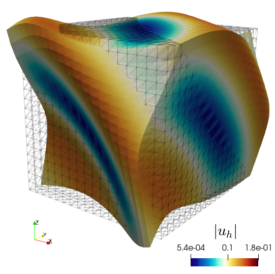
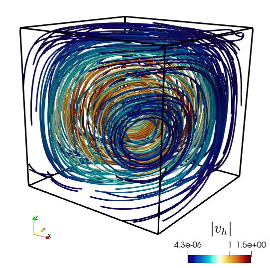
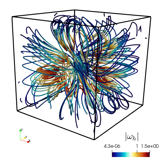
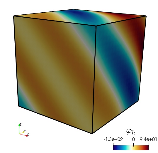
Next we conduct a second test of convergence, now in the unit cube domain $\Omega=(0,1)^{3}$ and with mixed boundary conditions (displacement, normal velocity and tangential vorticity are prescribed on the sides $x=0$ , $y=0$ , $z=0$ and known normal stress, flux, and pressures are imposed on the remainder of the boundary) considering closed-form solutions to the vorticity-based Biot–Brinkman equations as follows

	$\displaystyle\boldsymbol{u}(x,y,z)=\frac{1}{10}\begin{pmatrix}\sin(\pi[x+y+z])\\ \cos(\pi[x^{2}+y^{2}+z^{2}])\\ \sin(\pi[x+y+z])\cos(\pi[x+y+z])\end{pmatrix},\qquad p(x,y,z)=\sin(\pi x)\cos(\pi y)\sin(\pi z),$
	$\displaystyle\boldsymbol{v}(x,y,z)=\begin{pmatrix}\sin^{2}(\pi x)\sin(\pi y)\sin(2\pi z)\\ \sin(\pi x)\sin^{2}(\pi y)\sin(2\pi z)\\ -[\sin(2\pi x)\sin(\pi y)+\sin(\pi x)\sin(2\pi y)]\sin^{2}(\pi z)\end{pmatrix},\qquad\boldsymbol{\omega}(x,y,z)={\sqrt{\frac{\nu}{\kappa}}}\mathop{\mathbf{curl}}\nolimits\boldsymbol{v},\qquad\varphi(x,y,z)=-\lambda\mathop{\mathrm{div}}\nolimits\boldsymbol{u}+\alpha p.$

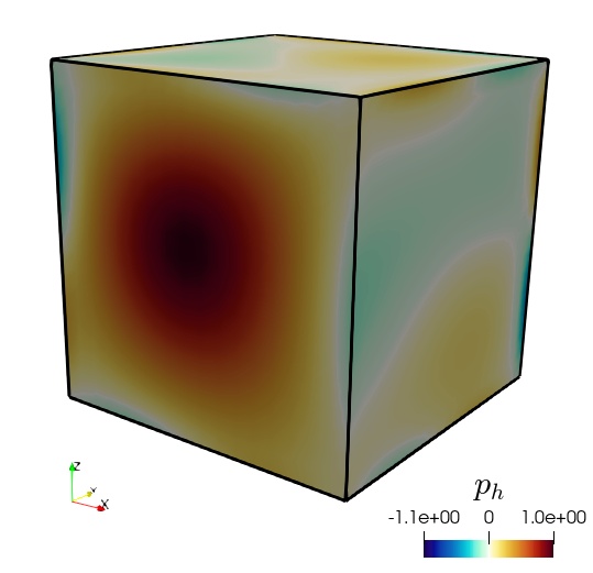
The 3D example uses generalised Taylor–Hood elements for the displacement/total pressure pair, but differently from (4.1), we take one polynomial degree higher for the approximation of velocity, vorticity and fluid pressure. This to maintain an overall $O(h^{k+2})$ convergence. This time we consider the parameter values $\nu=0.1$ , $\lambda=100$ , $\mu=10$ , $\kappa=10^{-3}$ , $c_{0}=0.1$ , $\alpha=0.1$ , and in Table 5.3 we only show the error decay measured in the total weighted norm that leads to the definition of $\mathcal{B}_{3}$ , that is $\|\vec{\boldsymbol{x}}-\vec{\boldsymbol{x}_{h}}\|_{\varepsilon}=\sqrt{(\vec{\boldsymbol{x}}-\vec{\boldsymbol{x}_{h}})\cdot\mathcal{B}_{3}^{-1}(\vec{\boldsymbol{x}}-\vec{\boldsymbol{x}_{h}})}$ . This shows an asymptotic $h^{k+2}$ order of convergence. For sake of illustration, we depict in Figure 5.1 the approximate solutions obtained after 4 levels of uniform refinement.

Refer to caption — Figure 5.1: Accuracy test in 3D. Approximate solutions of the Biot–Brinkman equations on a relatively coarse mesh. Displacements on the deformed configuration, velocity streamlines, vorticity vectors, total and fluid pressures computed with the lowest-order method.

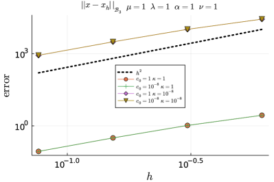
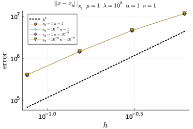
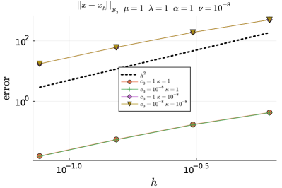
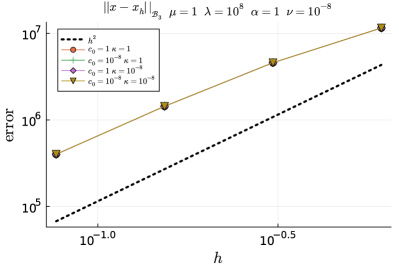
We also explore the dependence of the order of convergence upon variation of the base-line parameter values used in Table 5.3. We consider several sample values of model parameters $\mu\in[1,10^{8}]$ , $\lambda\in[1,10^{8}]$ , $\nu\in[10^{-6},1]$ , $\kappa\in[10^{-8},1]$ , $\alpha\in[0,1]$ , and $c_{0}\in[10^{-8},1]$ . These ranges are encountered in typical applications of poromechanics of subsurface flows and of linear Biot consolidation of soft tissues ^{16, 24, 43, 47, 56}. For the sake of brevity, however, we only report a subset of representative results we obtained with $\mu=1$ , $\alpha=1$ , $\lambda=\{1,10^{8}\}$ , $\nu=\{10^{-8},1\}$ , $\kappa=\{10^{-8},1\}$ , and $c_{0}=\{10^{-8},1\}$ . In any case, the software in ²¹ is written such that the reader might also run additional tests with other parameter values as per-required. We consider the unit cube domain discretised into uniform tetrahedral meshes. In particular, we consider four mesh resolutions, from one up to four levels of uniform refinement of the unit cube discretised with two tetrahedra. We use mixed boundary conditions, with $\Gamma$ being conformed by the faces $x=0$ , $y=0$ , $z=0$ and $\Sigma$ the remainder of the boundary.

The results are shown in Figure 5.2 for $k=0$ . Overall, the different convergence curves confirm $O(h^{k+2})$ convergence in the weighted norm that leads to the definition of $\mathcal{B}_{3}$ regardless of the parameter values, as predicted by the theoretical analysis.

5.3 Preconditioner robustness with respect to model parameters

Finally, we proceed to study the robustness of $\mathcal{B}_{j}^{-1}$ in (3.17) with respect to varying model parameters and increasing mesh resolution. We use the same combination of parameter values as in the previous section, namely $\mu=1$ , $\alpha=1$ , $\lambda=\{1,10^{8}\}$ , $\nu=\{10^{-8},1\}$ , $\kappa=\{10^{-8},1\}$ , and $c_{0}=\{10^{-8},1\}$ , and five levels of uniform refinement of the unit cube discretised with two tetrahedra. We used the same boundary conditions as in the previous section. We used the definition of FE spaces in (4.1) for $k=0$ . The action of the different inverses arising in the diagonal blocks of $\mathcal{B}_{j}^{-1}$ in (3.17) is implemented with the UMFPACK direct solver. For each combination of parameter values and mesh resolution, we used these preconditioners to accelerate the convergence of the MINRES iterative solver. Convergence is claimed whenever the Euclidean norm of the (unpreconditioned) residual of the whole system is reduced by a factor of $10^{6}$ , and stopped otherwise if the number of iterations reaches an upper bound of 500 iterations. The (discrete) Laplacian operator required for $\mathcal{B}_{2},\mathcal{B}_{3}$ acts on discontinuous pore pressure approximations so we use (for a given piecewise-defined field $\eta$ ) the following form (see ¹³)

\bigl{(}-\eta\Delta_{h}p_{h},q_{h}\bigr{)}_{0,\Omega}=\sum_{K\in\mathcal{T}_{h}}(\eta\nabla_{h}p_{h},\nabla_{h}p_{h})_{0,K}{+\sum_{e\in\mathcal{E}^{\mathrm{int}}_{h}}\bigl{\langle}\frac{\left\{\!\!\left\{\eta\right\}\!\!\right\}}{\left\{\!\!\left\{h_{e}\right\}\!\!\right\}}\left[\!\left[p_{h}\right]\!\right],\left[\!\left[q_{h}\right]\!\right]\bigr{\rangle}_{e}}+\sum_{e\in\mathcal{E}^{\Gamma}_{h}}\langle\frac{\eta}{h_{e}}{p_{h}},{q_{h}}\rangle_{e},

(5.2)

while for the lowest-order case we only keep the second and third terms on the right-hand side of (5.2).

In Figures 5.3-5.4 we show the number of preconditioned MINRES iterations versus number of DoFs for the $\mathcal{B}_{1}$ , $\mathcal{B}_{2}$ , and $\mathcal{B}_{3}$ preconditioners with the particular parameter value combinations mentioned above. Each of the plots in these figures contain 4 curves corresponding each to one of the four combinations of $\kappa=\{10^{-8},1\}$ , and $c_{0}=\{10^{-8},1\}$ . To facilitate the comparison among $\mathcal{B}_{1}$ , $\mathcal{B}_{2}$ , and $\mathcal{B}_{3}$ , the 6 plots in each figure are grouped into two groups of three horizontally adjacent plots each. Each group correspond to a combination of $\lambda=\{1,10^{8}\}$ , $\nu=\{10^{-8},1\}$ ; the particular combination corresponding to a group is indicated in the title of the three plots in the group.

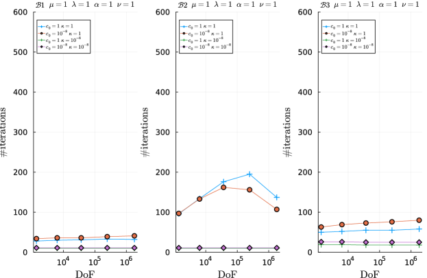
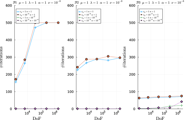
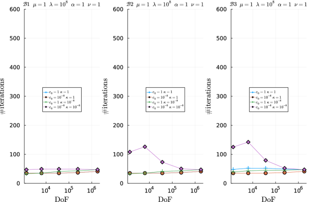
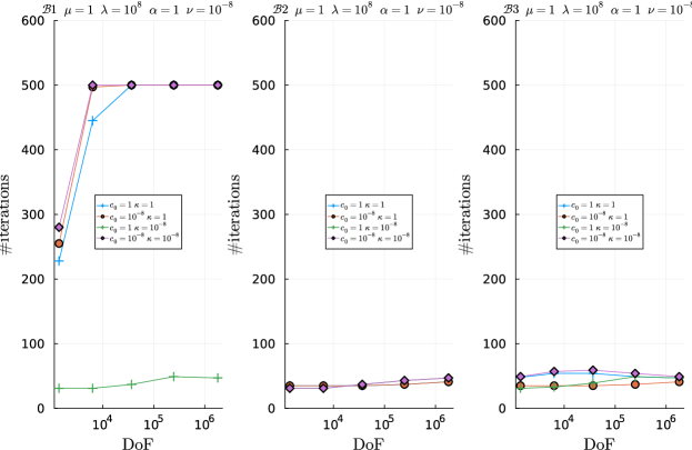
From Figures 5.3-5.4, we observe that the number of MINRES iterations with $\mathcal{B}_{3}$ reaches an asymptotically constant regime with increasing mesh resolution for all combinations of parameter values tested. This is also the case of $\mathcal{B}_{1}$ and $\mathcal{B}_{2}$ in the majority of cases, except for some combinations of parameter values in which $\nu=10^{-8}$ (see, e.g., $\mathcal{B}_{1}$ and $\mu=1$ , $\lambda=1$ , $\alpha=1$ , $\nu=10^{-8}$ , $\kappa=1$ , and $c_{0}=\{10^{-8},1\}$ ), where preconditioner efficiency (number of MINRES iterations) significantly degrades (increases) with mesh resolution. (We recall from Remark 4.9 that in the limit $\nu\rightarrow 0$ the system at hand becomes a four-field Biot system ¹⁶.) For these combinations of parameters, the coupling among the two pressures in the last leading block of $\mathcal{B}_{3}$ is essential to retain mesh independence convergence. This observation agrees with the experiments in ¹⁶ for four-field formulations of Biot poroelasticity and simpler problems (including Herrmann elasticity and reaction-diffusion equation), where comparisons were performed against sub-optimal preconditioners. On the other hand, we observe a relatively low sensitivity of the number of MINRES iterations (and thus robustness) with respect to the value of the model of parameters for all preconditioners (leaving aside the aforementioned combination of parameter values). For example, for $\mu=1$ , $\lambda=10^{8}$ , $\alpha=1$ , $\nu=10^{-8}$ , $\mathcal{B}_{3}$ , and finest mesh resolution, the number of iterations varies between 40 and 50 despite the disparity of scales in the values of $c_{0}$ and $\kappa$ . It is worth noting that $\mathcal{B}_{1}$ and $\mathcal{B}_{2}$ lead to a similar or even lower number of iterations than $\mathcal{B}_{3}$ in most cases, despite it being a computationally cheaper preconditioner. This is the case, e.g., for and $\mathcal{B}_{1}$ , $\mu=1$ , $\lambda=1$ , $\alpha=1$ , $\nu=1$ , and all combinations of $\kappa$ and $c_{0}$ tested.

6 Concluding remarks

We have presented a new formulation for the Biot–Brinkman problem using rescaled vorticity and total pressure, and have carried out the stability and solvability analysis of the continuous and discrete problems using parameter-weighted norms. We have derived theoretical error estimates and have subsequently confirmed them numerically; and we have constructed suitable preconditioners that achieve mesh-robustness iteration numbers when varying elastic and porous media flow model parameters. In order to be able to apply these algorithms to more realistic problems one needs to efficiently exploit the vast amount of hardware parallelism available in high-end supercomputers. As future work, we plan to address the parallelisation of the algorithms proposed using the GridapDistributed.jl package ¹².

Parts of the theoretical framework advanced herein (in particular, the use of a vorticity-based formulation for the filtration equation) extend naturally to more complex setups, for example to the multiple network generalised Biot–Brinkman model from ³⁵. Further improvements to the model and to the theory include the rigorous treatment of different types of boundary conditions, the interfacial coupling with free-flow or with elasticity, and robust a posteriori error estimates.

\bmsection

*Financial disclosure

None reported.

\bmsection

*Conflict of interest

The authors declare no potential conflict of interests.

References

1 M. Amara, D. Capatina-Papaghiuc, and D. Trujillo, Stabilized finite element method for Navier-Stokes equations with physical boundary conditions. Math. Comp., 76(259) (2007) 1195–1217.
2 M. Amara, E. Chacón Vera, and D. Trujillo, Vorticity–velocity–pressure formulation for Stokes problem. Math. Comp., 73(248) (2004) 1673–1697.
3 I. Ambartsumyan, E. Khattatov, I. Yotov, and P. Zunino, Simulation of flow in fractured poroelastic media: A comparison of different discretization approaches. In: I. Dimov, I. Faragó, and L. Vulkov (eds). Finite Difference Methods,Theory and Applications. FDM 2014. Lecture Notes in Computer Science, vol 9045. Springer, Cham (2015) 3–14.
4 V. Anaya, M. Bendahmane, D. Mora, and R. Ruiz-Baier, On a vorticity-based formulation for reaction-diffusion-Brinkman systems. Netw. Heterog. Media, 13(1) (2018) 69–94.
5 V. Anaya, A. Bouharguane, D. Mora, C. Reales, R. Ruiz-Baier, N. Seloula and H. Torres, Analysis and approximation of a vorticity-velocity-pressure formulation for the Oseen equations. J. Sci. Comput., 88(3) (2019) 1577–1606.
6 V. Anaya, R. Caraballo, B. Gómez-Vargas, D. Mora, and R. Ruiz-Baier, Velocity-vorticity-pressure formulation for the Oseen problem with variable viscosity. Calcolo, 58(4) (2021) e44(1–25).
7 V. Anaya, R. Caraballo, S. Caucao, L.F. Gatica, R. Ruiz-Baier, and I. Yotov, A vorticity-based mixed formulation for the unsteady Brinkman–Forchheimer equations. Comput. Methods Appl. Mech. Engrg., 404 (2023) e115829(1–30).
8 V. Anaya, G.N. Gatica, D. Mora, and R. Ruiz-Baier, An augmented velocity-vorticity-pressure formulation for the Brinkman equations. Int. J. Numer. Methods Fluids, 79(3) (2015) 109–137.
9 V. Anaya, D. Mora, R. Oyarzúa, and R. Ruiz-Baier, A priori and a posteriori error analysis of a mixed scheme for the Brinkman problem. Numer. Math., 133(4) (2016) 781–817.
10 S. Badia, A. F. Martín, and R. Planas, Block recursive LU preconditioners for the thermally coupled incompressible inductionless MHD problem. J. Comput. Phys., 274 (2014), 562–591.
11 S. Badia and F. Verdugo, Gridap: An extensible finite element toolbox in julia. J. Open Source Softw., 5 (2020), 2520.
12 S. Badia, A. F. Martín, and F. Verdugo, GridapDistributed: a massively parallel finite element toolbox in Julia, J. Open Source Softw., 7(74) (2022), 4157.
13 T. Bærland, M. Kuchta, K.-A. Mardal, and T. Thompson, An observation on the uniform preconditioners for the mixed Darcy problem, Numer. Methods PDEs, 36(6) (2020), 1718–1734.
14 C. Bernardi and N. Chorfi, Spectral discretization of the vorticity, velocity, and pressure formulation of the Stokes problem. SIAM J. Numer. Anal., 44(2) (2007) 826–850.
15 C. Bernardi, S. Dib, V. Girault, F. Hecht, F. Murat, and T. Sayah, Finite element methods for Darcy’s problem coupled with the heat equation. Numer. Math., 139 (2018) 315–348.
16 W. Boon, M. Kuchta, K.-A. Mardal, and R. Ruiz-Baier, Robust preconditioners and stability analysis for perturbed saddle-point problems – application to conservative discretizations of Biot’s equations utilizing total pressure, SIAM J. Sci. Comput., 43 (2021) B961–B983.
17 D. Braess, Stability of saddle point problems with penalty. RAIRO Modél. Math. Anal. Numér., 30 (1996) 731–742.
18 F. Brezzi and M. Fortin, Mixed and Hybrid Finite Element Methods. Springer-Verlag, 1991.
19 J. Brown, M. G. Knepley, D. A. May, L. C. McInnes, and B. Smith, Composable linear solvers for multiphysics, In 2012 11th International Symposium on Parallel and Distributed Computing, (2012) 55–62
20 R. Bürger, S. Kumar, D. Mora, R. Ruiz-Baier, and N. Verma, Virtual element methods for the three-field formulation of time-dependent linear poroelasticity. Adv. Comput. Math., 47 (2021) e2.
21 R. Caraballo, C. W. In, A. F. Martín, R. Ruiz-Baier, Software used in “Robust finite element methods and solvers for the Biot-Brinkman equations in vorticity form”, DOI: https://doi.org/10.5281/zenodo.10078398 (2023)
22 F.J. Carrillo and I.C. Bourg, Capillary and viscous fracturing during drainage in porous media. Phys. Rev. E, 103 (2021) e063106.
23 C.L. Chang, and B.-N. Jiang, An error analysis of least-squares finite element method of velocity-pressure-vorticity formulation for the Stokes problem. Comput. Methods Appl. Mech. Engrg., 84(3) (1990) 247–255.
24 S. Chen, Q. Hong, J. Xu, and K. Yang, Robust block preconditioners for poroelasticity. Comput. Methods Appl. Mech. Engrg., 369 (2020) e113229.
25 E. Chow, and M. A. Heroux, An object-oriented framework for block preconditioning. ACM Trans. Math. Softw., 24(2) (1998) 159–183.
26 E.C Cyr, J. N. Shadid, and R. S. Tuminaro, Teko: A Block Preconditioning Capability with Concrete Example Applications in Navier–Stokes and MHD. SIAM J. Sci. Comput., 38(5) (2016) S307–S331.
27 H.-Y. Duan and G.-P. Liang, On the velocity-pressure-vorticity least-squares mixed finite element method for the 3D Stokes equations. SIAM J. Numer. Anal., 41(6) (2003) 2114–2130.
28 F. Dubois, M. Salaün, and S. Salmon, First vorticity-velocity-pressure numerical scheme for the Stokes problem. Comput. Methods Appl. Mech. Engrg., 192(44–46) (2003) 4877–4907.
29 Y. Efendiev, J. Galvis, and Y. Vassilevski, Preconditioning of coupled systems and applications. Numer. Linear Alg. Appl., 16(7–8) (2009) 899–924.
30 A. Ern and J.-L. Guermond, Finite Elements I: Approximation and Interpolation. Vol. 72 of Texts in Applied Mathematics. Springer, Cham (2021).
31 G.N. Gatica, A Simple Introduction to the Mixed Finite Element Method. Theory and Applications. SpringerBriefs in Mathematics. Springer, Cham, 2014.
32 L. Giraud, C. Geuzaine, and J. Dominguez, An efficient preconditioner for elasto-poroelasticity based on the pressure-correction method. Int. J. Numer. Methods Engrg., 89(10) (2011) 1139–1164.
33 V. Girault and P.A. Raviart, Finite Element Methods for Navier–Stokes Equations. Theory and Algorithms. Springer, Berlin (1986).
34 M.-L. Hanot, An arbitrary order and pointwise divergence-free finite element scheme for the incompressible 3D Navier–Stokes equations. SIAM J. Numer. Anal., 61(2) (2023), 784–811.
35 Q. Hong, J. Kraus, M. Kuchta, M. Lymbery, K.-A. Mardal and M. E. Rognes, Robust approximation of generalized Biot-Brinkman problems, J. Sci. Comput., 93 (2022) e77.
36 Q. Hong, J. Kraus, M. Lymbery, and F. Philo, Conservative discretizations and parameter-robust preconditioners for Biot and multiple-network flux-based poroelasticity models, Numer. Linear Algebra Appl., 26 (2019) e2242.
37 S.K. Jha, Y Efendiev, J. Galvis, and Y. Vassilevski, Block-diagonal preconditioning for coupled systems in subsurface flow simulation. J. Comput. Phys., 299 (2015) 203–224.
38 G. Ju, M. Cai, J. Li, and J. Tian, Parameter-robust multiphysics algorithms for Biot model with application in brain edema simulation. Math. Comput. Simul., 177 (2020) 385–403.
39 R.C. Kirby, From functional analysis to iterative methods. SIAM Rev., 52(2) (2010) 269–293.
40 R.C. Kirby and L. Mitchell, Solver Composition Across the PDE/Linear Algebra Barrier. SIAM J. Sci. Comput. 40(1) (2018) C76–C98.
41 S. Kumar, R. Oyarzúa, R. Ruiz-Baier, and R. Sandilya, Conservative discontinuous finite volume and mixed schemes for a new four-field formulation in poroelasticity, ESAIM: Math. Model. Numer. Anal., 54 (2020) 273–299.
42 J. Lee, K.-A. Mardal, and R. Winther, Parameter-robust discretization and preconditioning of Biot’s consolidation model. SIAM J. Sci. Comput., 39 (2017) A1–A24.
43 J. J. Lee, E. Piersanti, K.-A. Mardal, and M. E. Rognes, A mixed finite element method for nearly incompressible multiple-network poroelasticity. SIAM J. Sci. Comput. 41 (2019) A722–A747.
44 P. Lenarda, M. Paggi, and R. Ruiz-Baier, Partitioned coupling of advection-diffusion-reaction systems and Brinkman flows. J. Comput. Phys., 344 (2017) 281–302.
45 X. Liu, Y. Zhang, and Z. Chen, A block-diagonal preconditioner for the solution of coupled PDEs in poromechanics. Numer. Methods PDEs, 36(4) (2020) 1407–1425.
46 K.-A. Mardal and R. Winther, Preconditioning discretizations of systems of partial differential equations, Numer. Linear Alg. Appl., 18 (2011) 1–40.
47 A. Mikelic, M.F. Wheeler, and T. Wick, Phase-field modeling of a fluid-driven fracture in a poroelastic medium. Comput. Geosci., 19(6) (2015) 1171–1195.
48 P. Monk, Finite Element Methods for Maxwell’s Equations, Oxford University Press, New York, 2003.
49 D. Orban, and A. S. Siqueira, LinearOperators.jl, DOI: https://doi.org/10.5281/zenodo.2559294 (2020)
50 R. Oyarzúa and R. Ruiz-Baier, Locking-free finite element methods for poroelasticity. SIAM J. Numer. Anal., 54 (2016) 2951–2973.
51 E. Piersanti, J.J. Lee, T. Thompson, K.-A. Mardal, and M.E. Rognes, Parameter robust preconditioning by congruence for multiple-network poroelasticity. SIAM J. S. Comput., 43 (2021) B984–B1007.
52 W. Qi, P. Seshaiyer, and J. Wang, Finite element method with the total stress variable for Biot’s consolidation model. Numer. Methods PDEs, 37(3) (2021) 2409–2428.
53 A. Quarteroni, Numerical Models for Differential Problems. Springer-Verlag Milano (2009).
54 K.R. Rajagopal, On a hierarchy of approximate models for flows of incompressible fluids through porous solids. Math. Model. Methods Appl. Sci., 17 (2007) 215–252.
55 E. Rohan, J. Turjanicová, and V. Lukeš, The Biot–Darcy–Brinkman model of flow in deformable double porous media; homogenization and numerical modelling. Comput. Math. Appl., 78 (2019) 3044–3066.
56 R. Ruiz-Baier, M. Taffetani, H.D. Westermeyer, and I. Yotov, The Biot–Stokes coupling using total pressure: formulation, analysis and application to interfacial flow in the eye. Comput. Methods Appl. Mech. Engrg., 389 (2022) e114384.
57 M. Salaün, and S. Salmon, Low-order finite element method for the well-posed bidimensional Stokes problem. IMA J. Numer. Anal., 35 (2015) 427–453.
58 N. Verma, B. Gómez-Vargas, L. M. De Oliveira Vilaca, S. Kumar, and R. Ruiz-Baier, Well-posedness and discrete analysis for advection-diffusion-reaction in poroelastic media, Appl. Anal., 101(14) (2022) 4914–4941.
59 J. Zhang, C. Zhou, Y. Cao, and A.J. Meir, A locking free numerical approximation for quasilinear poroelasticity problems. Comput. Math. Appl., 80(16) (2020) 1538–1554.

	$\displaystyle a_{1}(\boldsymbol{u},\boldsymbol{\gamma})\leq 2\mu\|\boldsymbol{u}\|_{1,\Omega}\|\boldsymbol{\gamma}\|_{1,\Omega},\qquad b_{1}(\boldsymbol{\gamma},\varphi)\leq\\|\varphi\\|_{0,\Omega}\|\boldsymbol{\gamma}\|_{1,\Omega},\qquad\hat{b}_{1}(\boldsymbol{\zeta},q)\leq\\|q\\|_{0,\Omega}\\|\mathop{\mathrm{div}}\nolimits\boldsymbol{\zeta}\\|_{0,\Omega},$
	$\displaystyle a_{2}(\boldsymbol{v},\boldsymbol{\zeta})\leq\dfrac{1}{\kappa}\\|\boldsymbol{v}\\|_{0,\Omega}\\|\boldsymbol{\zeta}\\|_{0,\Omega}+\dfrac{\nu}{\kappa}\\|\mathop{\mathrm{div}}\nolimits\boldsymbol{v}\\|_{0,\Omega}\\|\mathop{\mathrm{div}}\nolimits\boldsymbol{\zeta}\\|_{0,\Omega},\qquad b_{2}(\boldsymbol{\theta},\boldsymbol{\zeta})\leq\sqrt{\frac{\nu}{\kappa}}\\|\mathop{\mathrm{curl}}\nolimits\boldsymbol{\theta}\\|_{0,\Omega}\\|\boldsymbol{\zeta}\\|_{0,\Omega},$
	$\displaystyle a_{3}(\boldsymbol{\omega},\boldsymbol{\theta})\leq\\|\boldsymbol{\omega}\\|_{0,\Omega}\\|\boldsymbol{\theta}\\|_{0,\Omega},\qquad a_{4}(\varphi,\psi)\leq\dfrac{1}{\lambda}\\|\varphi\\|_{0,\Omega}\\|\psi\\|_{0,\Omega},$
	$\displaystyle b_{3}(q,\psi)\leq\frac{\alpha}{\lambda}\\|q\\|_{0,\Omega}\\|\psi\\|_{0,\Omega},\qquad a_{5}(p,q)\leq\left(c_{0}+\dfrac{\alpha^{2}}{\lambda}\right)\\|p\\|_{0,\Omega}\\|q\\|_{0,\Omega},$		(3.5)

	$\displaystyle\langle\mathcal{A}_{\epsilon}(\vec{\boldsymbol{z}}),\vec{\boldsymbol{y}}\rangle$	$\displaystyle=2\mu\|\boldsymbol{\gamma}\|_{1,\Omega}^{2}+\dfrac{1}{\kappa}\\|\boldsymbol{\zeta}\\|_{0,\Omega}^{2}+\dfrac{\sqrt{\nu}}{2\sqrt{\kappa}}(\boldsymbol{\zeta},\mathop{\mathbf{curl}}\nolimits\boldsymbol{\theta})_{0,\Omega}+\dfrac{\nu}{\kappa}\\|\mathop{\mathrm{div}}\nolimits\boldsymbol{\zeta}\\|_{0,\Omega}^{2}+\dfrac{\nu}{2}\\|\mathop{\mathbf{curl}}\nolimits\boldsymbol{\theta}\\|_{0,\Omega}^{2}$
		$\displaystyle\qquad+\\|\boldsymbol{\theta}\\|_{0,\Omega}^{2}+\dfrac{1}{\lambda}\\|\psi\\|_{0,\Omega}^{2}-\dfrac{\alpha}{\lambda}(q,\psi)_{0,\Omega}-\dfrac{\alpha}{\lambda}(q,\psi)+\left(c_{0}+\dfrac{\alpha^{2}}{\lambda}\right)\\|q\\|_{0,\Omega}^{2}$
		$\displaystyle\geq 2\mu\|\boldsymbol{\gamma}\|_{1,\Omega}^{2}+\dfrac{1}{\kappa}\\|\boldsymbol{\zeta}\\|_{0,\Omega}^{2}+\dfrac{\sqrt{\nu}}{2\sqrt{\kappa}}(\boldsymbol{\zeta},\mathop{\mathbf{curl}}\nolimits\boldsymbol{\theta})_{0,\Omega}+\dfrac{\nu}{\kappa}\\|\mathop{\mathrm{div}}\nolimits\boldsymbol{\zeta}\\|_{0,\Omega}^{2}+\dfrac{\nu}{2}\\|\mathop{\mathbf{curl}}\nolimits\boldsymbol{\theta}\\|_{0,\Omega}^{2}+\\|\boldsymbol{\theta}\\|_{0,\Omega}^{2}$
		$\displaystyle\qquad+\left(c_{0}+\dfrac{\alpha^{2}}{\lambda}-\dfrac{\varepsilon\alpha}{2\lambda}\right)\\|q\\|_{0,\Omega}^{2}+\left(\dfrac{1}{\lambda}-\dfrac{\alpha}{2\lambda\varepsilon}\right)\\|\psi\\|_{0,\Omega}^{2}.$

	$\displaystyle\\|\vec{\boldsymbol{y}}\\|_{\mathbf{X}}^{2}$	$\displaystyle=2\mu\|\boldsymbol{\gamma}\|_{1,\Omega}^{2}+\frac{1}{\kappa}\left\\|\boldsymbol{\zeta}+\dfrac{\sqrt{\kappa\nu}}{2}\mathop{\mathbf{curl}}\nolimits\boldsymbol{\theta}\right\\|_{0,\Omega}^{2}+{\dfrac{\nu}{\kappa}}\\|\mathop{\mathrm{div}}\nolimits\boldsymbol{\zeta}\\|_{0,\Omega}^{2}+\nu\\|\mathop{\mathbf{curl}}\nolimits\boldsymbol{\theta}\\|_{0,\Omega}^{2}+\\|\boldsymbol{\theta}\\|_{0,\Omega}^{2}+\left(c_{0}+\dfrac{\alpha^{2}}{\lambda}\right)\\|q\\|_{0,\Omega}^{2}+\dfrac{1}{\lambda}\\|\psi\\|_{0,\Omega}^{2}$
		$\displaystyle\leq 2\mu\|\boldsymbol{\gamma}\|_{1,\Omega}^{2}+\dfrac{2\nu}{\kappa}\\|\boldsymbol{\zeta}\\|_{0,\Omega}^{2}+{\dfrac{\nu}{\kappa}}\\|\mathop{\mathrm{div}}\nolimits\boldsymbol{\zeta}\\|_{0,\Omega}^{2}+\dfrac{3\nu}{2}\\|\mathop{\mathbf{curl}}\nolimits\boldsymbol{\theta}\\|_{0,\Omega}^{2}+\\|\boldsymbol{\theta}\\|_{0,\Omega}^{2}+\left(c_{0}+\dfrac{\alpha^{2}}{\lambda}\right)\\|q\\|_{0,\Omega}^{2}+\dfrac{1}{\lambda}\\|\psi\\|_{0,\Omega}^{2}$
		$\displaystyle\leq 2\\|\vec{\boldsymbol{z}}\\|_{\mathbf{X}}^{2},$

	$\displaystyle\langle\mathcal{A}_{\epsilon}(\vec{\boldsymbol{x}}),10\vec{\boldsymbol{y}}_{1}+\delta\vec{\boldsymbol{y}}_{2}+\hat{\delta}\vec{\boldsymbol{y}}_{3}\rangle$	$\displaystyle\geq\\|\vec{\boldsymbol{x}}\\|^{2}_{\mathbf{X}}+\delta(a_{2}(\boldsymbol{v},\boldsymbol{\zeta}_{2})+b_{2}(\boldsymbol{\omega},\boldsymbol{\zeta}_{2})+\hat{b}_{1}(\boldsymbol{\zeta}_{2},p))+\hat{\delta}(a_{1}(\boldsymbol{u},\boldsymbol{\gamma}_{3})+b_{1}(\boldsymbol{\gamma}_{3},\varphi))$
		$\displaystyle\geq\\|\vec{\boldsymbol{x}}\\|^{2}_{\mathbf{X}}-\delta\left\{\dfrac{1}{\kappa}\\|\boldsymbol{v}\\|_{0,\Omega}+\dfrac{\nu}{\kappa}\\|\mathop{\mathrm{div}}\nolimits\boldsymbol{v}\\|_{0,\Omega}^{2}\right\}^{1/2}\left\{\dfrac{1}{\kappa}\\|\boldsymbol{\zeta}_{2}\\|_{0,\Omega}+\dfrac{\nu}{\kappa}\\|\mathop{\mathrm{div}}\nolimits\boldsymbol{\zeta}_{2}\\|_{0,\Omega}^{2}\right\}^{1/2}$
		$\displaystyle\qquad-\delta\dfrac{\nu}{\sqrt{\kappa}}\\|\mathop{\mathrm{curl}}\nolimits\boldsymbol{\omega}\\|_{0,\Omega}\\|\boldsymbol{\zeta}_{2}\\|_{0,\Omega}+\delta C_{1}\\|p\\|_{r}^{2}-2\mu\hat{\delta}\|\boldsymbol{u}\|_{1,\Omega}\|\boldsymbol{\gamma}_{3}\|_{1,\Omega}+\hat{\delta}\frac{\hat{C}_{1}}{2\mu}\\|\varphi\\|_{0,\Omega}^{2}$
		$\displaystyle\geq\\|\vec{\boldsymbol{x}}\\|^{2}_{\mathbf{X}}-\dfrac{1}{2}\left(\dfrac{1}{\kappa}\\|\boldsymbol{v}\\|_{0,\Omega}+\dfrac{\nu}{\kappa}\\|\mathop{\mathrm{div}}\nolimits\boldsymbol{v}\\|_{0,\Omega}^{2}\right)-\dfrac{\nu}{2}\\|\mathop{\mathrm{curl}}\nolimits\boldsymbol{\omega}\\|_{0,\Omega}^{2}-\mu\|\boldsymbol{u}\|_{1,\Omega}^{2}+\delta C_{1}\\|p\\|_{r}^{2}$
		$\displaystyle\qquad+\hat{\delta}\frac{\hat{C}_{1}}{2\mu}\\|\varphi\\|_{0,\Omega}^{2}-\delta^{2}\dfrac{1}{\kappa}\\|\boldsymbol{\zeta}_{2}\\|_{0,\Omega}-\delta^{2}\dfrac{\nu}{2\kappa}\\|\mathop{\mathrm{div}}\nolimits\boldsymbol{\zeta}_{2}\\|_{0,\Omega}^{2}-2\mu\hat{\delta}^{2}\|\boldsymbol{\gamma}_{3}\|_{1,\Omega}^{2}$
		$\displaystyle\geq\dfrac{1}{2}\\|\vec{\boldsymbol{x}}\\|^{2}_{\mathbf{X}}+\delta(C_{1}-\delta C_{2}^{2})\\|p\\|_{r}^{2}+\hat{\delta}\frac{1}{2\mu}\left(\hat{C}_{1}-\hat{\delta}\hat{C_{2}}^{2}\right)\\|\varphi\\|_{0,\Omega}^{2}.$

	$\displaystyle\langle\mathcal{A}_{\epsilon}(\vec{\boldsymbol{x}}),10\vec{\boldsymbol{y}}_{1}+\delta\vec{\boldsymbol{y}}_{2}+\hat{\delta}\vec{\boldsymbol{y}}_{3}\rangle$	$\displaystyle\geq\dfrac{1}{2}\\|\vec{\boldsymbol{x}}\\|^{2}_{\mathbf{X}}+\dfrac{C_{1}^{2}}{4C_{2}^{2}}\\|p\\|_{r}^{2}+\dfrac{\hat{C}_{1}^{2}}{4\hat{C}_{2}^{2}}\frac{1}{2\mu}\\|\varphi\\|_{0,\Omega}^{2}\geq\dfrac{1}{2}\min\left\{1,\dfrac{C_{1}^{2}}{2C_{2}^{2}},\dfrac{\hat{C}_{1}^{2}}{2\hat{C}_{2}^{2}}\right\}\\|\vec{\boldsymbol{x}}\\|^{2}_{\epsilon},\qquad\text{and}$
	$\displaystyle\\|10\vec{\boldsymbol{y}}_{1}+\delta\vec{\boldsymbol{y}}_{2}+\hat{\delta}\vec{\boldsymbol{y}}_{3}\\|_{\epsilon}$	$\displaystyle\leq 10\sqrt{2}\\|\vec{\boldsymbol{x}}\\|_{\epsilon}+\delta C_{2}\\|p\\|_{r}+\hat{\delta}\hat{C}_{2}\frac{1}{\sqrt{2\mu}}\\|\varphi\\|_{0,\Omega}\leq\max\left\{10\sqrt{2},\dfrac{C_{1}}{2C_{2}},\dfrac{\hat{C}_{1}}{2\hat{C}_{2}}\right\}\\|\vec{\boldsymbol{x}}\\|_{\epsilon}.$