mystyle2\captionlabel. \captiontext \captionstylemystyle2
Robust Design for IRS-Aided Communication Systems with User Location Uncertainty
Abstract
In this paper, we propose a robust design framework for IRS-aided communication systems in the presence of user location uncertainty. By jointly designing the transmit beamforming vector at the BS and phase shifts at the IRS, we aim to minimize the transmit power subject to the worse-case quality of service (QoS) constraint, i.e., ensuring the user rate is above a threshold for all possible user location error realizations. With unit-modulus, this problem is not convex. The location uncertainty in the QoS constraint further increases the difficulty of solving this problem. By utilizing techniques of Taylor expansion, S-Procedure and semidefinite relaxation (SDP), we transform this problem into a sequence of semidefinite programming (SDP) sub-problems. Simulation results show that the proposed robust algorithm substantially outperforms the non-robust algorithm proposed in the literature, in terms of probability of reaching the required QoS target.
Index Terms:
IRS, robust beamforming, SDP.Robust design for an IRS-aided system under user location uncertainty
I Introduction
Intelligent reflecting surface (IRS) has recently emerged as a promising method to tackle the coverage problem of dead-zone users [1, 2]. The IRS is a meta-surface consisting of a large number of low-cost, passive reflecting elements, each of which can independently reflect the incident signal with adjustable phase shifts. Through proper design of the phase shifts at the IRS [3, 4], the signal received at the user can be significantly enhanced.
To facilitate the design of phase shifts, channel state information (CSI) is compulsory. As such, plenty of works have been devoted to the estimation of IRS-aided channels, including the channel between the BS and IRS, as well as the reflection channel between the IRS and user. In general, the proposed methods can be categorized into two types. The first type is to estimate the cascaded channels[5, 6]. However, with a large number of reflecting elements, the training overhead would become prohibitive. The second type is to directly estimate two channels separately [7], assuming that the IRS has both reflection mode and receive mode. However, this requires a large number of receive radio frequency (RF) chains (equal to the number of reflecting elements), which would significantly increase the hardware cost as well as the power consumption of the IRS.
To tackle the above issues, one possible way is to only estimate the angles of arrivals (AOAs) and angles of departures (DOAs)[8, 9, 10]. Because the locations of the IRS and BS remain fixed, the channel between the BS and IRS varies very slowly and can be accurately estimated by computing the AOAs and AODs [11]. Then, exploiting the user location information provided, for example, by global positioning system (GPS), the angular information of the reflection channel from the IRS to the user can be obtained. However, due to user mobility and the precision of GPS, the user location information may not be accurate, resulting in imperfect angular information.
Motivated by this, this letter proposes a robust design framework in the presence of user location uncertainty.111 Unlike [11] and [12], which adopt conventional error model, the current work first proposes a location-based channel estimation scheme, and then presents a practical channel error model related to location uncertainty. In addition, the method to tackle the optimization problem is also different from [11] and [12]. Specifically, considering a bounded spherical error model, the transmit beamforming vector and phase shifts are jointly designed to minimize the transmit power, subject to the minimum achievable rate constraint for all possible user location errors. To tackle the non-convex worse-case rate constraint, the second-order Taylor expansion is used to approximate the achievable rate, and the S-Procedure is used to convert the resultant semi-definite constraint into a matrix inequality. Then, applying the semi-definite relaxation (SDR) method, an alternating algorithm is designed, which optimizes the transmit beamforming vector and phase shifts iteratively by solving a sequence of semi-definite programming (SDP) sub-problems. Simulation results show that the proposed robust algorithm can guarantee the target rate regardless of the user location errors, which substantially outperforms the non-robust algorithm proposed in [3].
II System Model
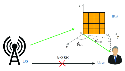
We consider an IRS-aided system as illustrated in Fig.1, where one BS with antennas communicates with a single-antenna user, which is assisted by an IRS with reflecting elements. Like most works on IRS, e.g.,[3, 5], we assume that the IRS operates in the far-field regime. Furthermore, we assume that direct link between the BS and the user does not exist, due to blockage or unfavorable propagation environments. Both the BS and the IRS are equipped with uniform rectangular arrays (URAs) with the size of and respectively, where () and () denote the numbers of BS antennas and reflecting elements along the () axis, respectively.
II-A Downlink Transmission
During the downlink data transmission phase, the BS transmits the signal , where is the beamforming vector and is the symbol for the user, satisfying .
Then, the signal received at the user is given by
| (1) |
where denotes the channel from the IRS to the user, is the channel between the BS and the IRS, and is the additive white Gaussian noise (AWGN) which follows the circularly symmetric complex Gaussian distribution with zero mean and variance . The phase shift matrix of the IRS is given by with the phase shift beam .
II-B Channel Model
We consider a narrowband millimeter-wave (mmWave) system, and adopt the narrowband geometric channel model. As such, the channel from the IRS to the BS can be expressed as
| (2) |
where is the number of paths, is the channel coefficient of the -th path, and are the array response vectors of the BS and IRS respectively. The effective angles of departure (AODs) of the -th path, i.e., the phase differences between two adjacent antennas along and axes, are given by and , respectively, where is the distance between two adjacent BS antennas, is the carrier wavelength, and are the elevation and azimuth AODs, respectively. Similarly, the two effective angles of arrival (AOAs) can be written as and , respectively, where is the distance between two adjacent reflecting elements, and are the elevation and azimuth AOAs, respectively. We further assume that .
The -th element of and the -th element of are respectively given by
| (3) | |||
| (4) | |||
| (5) | |||
| (6) |
where , and we use to denote the -th entry of a vector .
Since the IRS is usually deployed near the user, a LOS channel model is assumed to model the reflection channel between the IRS and the user. Specifically, the channel from the IRS to the user is given by
| (7) |
where is the channel coefficient, the two effective AODs from the IRS to the user and are respectively defined as [15]
| (8) | |||
| (9) |
where and are respectively the elevation and azimuth AODs, as shown in Fig. 1.
II-C Performance Measure
Assuming Gaussian signaling, the achievable rate of the system can be expressed as
| (10) |
III Location-Based Channel Estimation
In the IRS-aided communication system, due to the fixed location of the IRS, the channel from the BS to the IRS, i.e., , usually remains constant over a long period, and thus can be accurately estimated. Therefore, we assume that is perfectly known. In contrast, due to user mobility, the reflection channel varies over the time, hence should be estimated. As such, we propose to exploit user location information to estimate the reflection channel .
The elevation and azimuth AODs ( and ) have the following relationship with the locations of the IRS and user:
| (11) |
where is the distance between the IRS and the user, and are locations of the IRS and the user respectively. Substituting (11) into (8) and (9), we obtain the relationship between the effective AODs ( and ) and locations of the IRS and the user:
| (12) |
In general, user location information obtained from the GPS is imperfect. Let denote the estimated location of the user and denote the estimation error. The estimated effective AODs from the IRS to the user are given by
| (13) |
Proposition 1.
The effective AODs from the IRS to the user can be approximately decomposed as
| (14) |
where
where denotes the accurate location of the user, , , and are location errors along , and axes, respectively.
Proof.
Starting from (13), we can obtain the desired result. ∎
Invoking the results given by Proposition 1, the reflection channel can be expressed as
| (15) |
where stands for Hadamard product, is the estimated channel, and is the estimation error with , where with
| (16) | |||
| (17) |
| (18) | |||
| (19) |
IV Robust Beamforming Design
Assuming that the location error is bounded by a sphere with the radius , i.e.,, we aim to minimize the total transmit power through joint design of beamforming vector and phase shift vector under the worst-case QoS constraint, namely, the achievable rate should be above a threshold . Mathematically, the worst-case robust design problem can be formulated as
| (20) | ||||
IV-A Problem Transformation
Denote and . The robust constraint in (21) is reformulated as
| (25) |
Constraint (25) is a non-convex constraint involving infinitely many inequality constraints due to the continuity of the location uncertainty set. To handle the infinite inequalities, we give an approximation of the left hand side of (25), which is shown in the following proposition.
Proposition 2.
The left hand side of (25) can be approximated as where , , with representing the entry in the -th row and the -th column of and .
Proof.
By applying second-order Taylor expansion, we can obtain the desired result. ∎
Based on Proposition 2, (25) can be rewritten as
| (26) |
Then, we leverage the following lemma to convert constraint (26) into an equivalent form involving one matrix inequality.
Lemma 1.
(General S-Procedure) Consider the quadratic matrix inequality (QMI)[13]:
| (27) | |||
where represents the trace, with being the set of Hermitain matrices, and . This QMI holds if there exists such that
| (28) |
provided that there exists a point such that .
The transformed constraint (29) involves only one matrix inequality constraint, which is more amenable for algorithm design compared to the infinitely many constraints in the original constraint (25). However, the resulting optimization problem is still not jointly convex with respect to and . Therefore, we adopt an alternating optimization method to optimize and iteratively.
IV-B Optimization of
Specifically, for given phase shift beam , the sub-problem of problem (21) corresponding to the beamforming vector is formulated as
| (32) |
However, the constraint (29) is non-convex. To proceed, we recast the optimization problem as a rank-constrained SDP problem. By applying the change of variables , problem (32) can be rewritten as
| (33) | |||
| (36) |
where denotes the set of positive semidefinite Hermitain matrices, , , , where denotes a vector whose elements all equal to 1, , and with entries in the -th row and the -th column given by and .
As such, the only remaining non-convexity of problem (14) is due to the rank constraint. Generally, solving such a rank-constrained problem is known to be NP-hard. To overcome this issue, we adopt the SDR technique and drop the rank constraint.
| (37) | ||||
| (39) |
Therefore, the resulting problem becomes a convex SDP problem, and thus can be efficiently solved by standard convex program solvers such as CVX. While there is no guarantee that the solution obtained by SDR satisfies the rank constraint, the Gaussian randomization can be used to obtain a feasible solution to problem (32) based on the higher-rank solution obtained by solving (37).
IV-C Optimization of
For given beamforming vector , the sub-problem of problem (21) corresponding to the phase shift beam becomes a feasibility-check problem. To further improve optimization performance, we introduce a slack variable , which is interpreted as the “SINR residual” of the user. Hence, the feasibility-check problem of is formulated as follows
| (40) | ||||
where the Modified-(29) is obtained from (29) by replacing with .
To address the non-convexity of both the constraint (29) and the unit-modulus constraint, we apply change of variables . Hence, the problem (40) can be transformed into a rank-constrained (SDP) problem as follows:
| (41) | ||||
| (45) |
where , , , and .
To handle the non-convexity of the rank constraint in (41), we adopt the SDR technique and drop the rank constraint.
| (46) | ||||
| (49) |
IV-D Alternating Optimization of and
Problem (20) is tackled by solving two sub-problems (37) and (46) in an iterative manner, the details of which are summarized in Algorithm 1.
Remark 1.
Note that all considered sub-problems are SDP problems, which can be solved by interior point method. Therefore, the approximate complexity of problem (37) is , and that of problem (46) is . Finally, the approximate complexity of Algorithm 2 per iteration is . With such complexity, it is required that the BS has strong computational capacity so that the transmit beam and IRS phase shifts can be computed in real time.
Remark 2.
Since a SDR technique followed by Gaussian randomization is adopted when solving the two sub-problems, the strict convergence of the proposed alternating algorithm can not be guaranteed. But for each sub-problem, such a SDR approach followed by a sufficiently large number of randomizations guarantees at least a -approximation of the optimal objective value.
V Simulation results
In this section, we provide numerical results to evaluate the performance of the proposed algorithm. The considered system is assumed to operate at GHz with bandwidth of 100 MHz and noise spectral power density of -169 dBm/Hz. The IRS is at the origin of a Cartesian coordinate system. The locations of the BS and the user are and , respectively. Unless otherwise specified, the following setup is used: , and .222As pointed out in [16], synchronously operating a large number of phase shifters is a non-trivial task. The IRS may suffer from phase errors. It have been shown in [17] that the average received SNR is attenuated by where with being the phase error. One possible way to reduce the phase error is to use phase shifters with adaptive tuning capability.
Fig. 2 compares the proposed robust scheme with a “Non-robust” optimization scheme [3]. It is worth noting that the target rate is a predefined threshold, while the x-axis in Fig.2 () is the rate achieved under different location errors of each channel realization. The proposed robust beamforming scheme requires that the achievable rate under all possible location errors should exceed the threshold , while the non-robust beamforming scheme regards the estimated channels as perfect channels, and aims to maximize the achievable rate without location uncertainty, using the same power as the proposed beamforming scheme. As can be readily seen, the variation of the user rate with robust optimization is much smaller than that with non-robust optimization. Moreover, the target rate can be always guaranteed regardless of user location errors. By contrast, with non-robust optimization, the user rate varies over a wide range. For instance, with , the user rate ranges from near 0 bits/s/Hz to about 7.2 bits/s/Hz. Moreover, there is a high probability (over ) that the target rate can not be achieved.
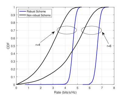
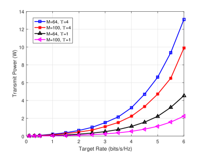
Fig. 3 presents the transmit power versus the target rate with different location uncertainty and numbers of reflecting elements. Obviously, to achieve a higher target rate, more power is required. Also, as location uncertainty (measured by ) increases, the required transmit power becomes larger so that the target rate can be achieved for all possible location errors. Besides, since both the beamforming gain and the aperture gain of the IRS grow with the number of reflecting elements, the transmit power drops significantly with the number of reflecting elements, implying the benefit of the IRS in power saving.
VI Conclusion
In this paper, considering user location uncertainty, we study the robust beamforming design for an IRS-aided communication system. We first handle the location uncertainty by exploiting techniques of Taylor expansion and S-Procedure. Then SDR is used to transform the non-convex problem into a sequence of SDP sub-problems, which can be efficiently solved via some optimization tools, for example, CVX. Simulation results demonstrate that with our proposed robust algorithm, the QoS requirement is always met regardless of location uncertainty, while with a non-robust optimization algorithm [3] which has the same transmit power as the proposed algorithm, the QoS requirement is met with a probability below .
References
- [1] S. Dang, O. Amin, B. Shihada, and M. Alouini, “What should 6G be?” Nature Electronics, vol. 3, pp. 20–29, 2020.
- [2] Q. Wu and R. Zhang, “Towards smart and reconfigurable environment: intelligent reflecting surface aided wireless network,” IEEE Commun. Mag., vol. 58, no. 1, pp. 106–112, Jan. 2020.
- [3] Q. Wu and R. Zhang, “Intelligent reflecting surface enhanced wireless network via joint active and passive beamforming,” IEEE Trans. Commun., vol. 18, no. 11, pp. 5394–5409, 2019.
- [4] X. Hu, C. Zhong, Y. Zhu, X. Chen, and Z. Zhang, “Programmable metasurface based multicast systems: Design and analysis,” IEEE J. Selected Areas Commun., vol. 38, no. 8, pp. 1763-1776, Aug. 2020.
- [5] B. Zheng and R. Zhang, “Intelligent reflecting surface-enhanced OFDM: Channel estimation and reflection optimization,” IEEE Wireless Commun. Lett., vol. 9, no. 4, pp. 518–522, Apr. 2020.
- [6] Z. He and X. Yuan, “Cascaded channel estimation for large intelligent metasurface assisted massive MIMO,” IEEE Wireless Commun. Lett., vol. 9, no. 2, pp. 210–214, Feb. 2020.
- [7] A. Taha, M. Alrabeiah, and A. Alkhateeb, “Enabling large intelligent surfaces with compressive sensing and deep learning,” [Online]. Available: https://arxiv.org/abs/1904.10136.
- [8] X. Hu, C. Zhong, Y. Zhang, X. Chen, and Z. Zhang, “Location information aided multiple intelligent reflecting surface systems,” accepted to appear in IEEE Trans. Commun., 2020.
- [9] Y. Han, W. Tang, S. Jin, C.-K. Wen, and X. Ma, “Large intelligent surface-assisted wireless communication exploiting statistical CSI, ”IEEE Trans. Veh. Technol., vol. 68, no. 8, pp. 8238–8242, 2019.
- [10] X. Hu, J. Wang, and C. Zhong, “Statistical CSI based design for intelligent reflecting surface assisted MISO systems,” accepted to appear in Science China: Information Science, 2021.
- [11] G. Zhou, C. Pan, H. Ren, K. Wang, M. Di Renzo, and A. Nallanathan, “Robust beamforming design for intelligent reflecting surface aided MISO communication systems,” [Online]. Available: https://arxiv.org/abs/1911.06237.
- [12] J. Zhang, Y. Zhang, C. Zhong and Z. Zhang, “Robust design for intelligent reflecting surfaces assisted MISO systems,” IEEE Commun. Lett., Early Access, doi: 10.1109/LCOMM.2020.3002557.
- [13] Z.-Q. Luo, J. F. Sturm, and S. Zhang, “Multivariate nonnegative quadratic mappings,” SIAM Journal on Optimization, vol. 14, no. 4, pp. 1140–1162, 2004.
- [14] A. Ben-Tal and A. Nemirovski, Lectures on modern convex optimization: analysis, algorithms, and engineering applications. Siam, 2001, vol. 2.
- [15] H. L. V. Trees,Detection, Estimation, and Modulation Theory: Optimum Array Processing. Wiley, 2002.
- [16] H. Tataria, F. Tufvesson, and O. Efors, “Real-Time implementation aspects of large intelligent surfaces,” ICASSP 2020 - 2020 IEEE International Conference on Acoustics, Speech and Signal Processing (ICASSP), Barcelona, Spain, 2020, pp. 9170-9174.
- [17] M.-A. Badiu, and J. P. Coon, “Communication through a large reflecting surface with phase errors,” IEEE Wireless Commun. Lett., vol. 9, no. 2, pp. 184–188, Feb. 2020.