Robust Control Lyapunov-Value Functions for Nonlinear Disturbed Systems

Zheng Gong [email protected] Sylvia Herbert [email protected] La Jolla, San Diego

Abstract

Control Lyapunov Functions (CLFs) have been extensively used in the control community. A well-known drawback is the absence of a systematic way to construct CLFs for general nonlinear systems, and the problem can become more complex with input or state constraints. Our preliminary work on constructing Control Lyapunov Value Functions (CLVFs) using Hamilton-Jacobi (HJ) reachability analysis provides a method for finding a non-smooth CLF. In this paper, we extend our work on CLVFs to systems with bounded disturbance and define the Robust CLVF (R-CLVF). The R-CLVF naturally inherits all properties of the CLVF; i.e., it first identifies the ”smallest robust control invariant set (SRCIS)” and stabilizes the system to it with a user-specified exponential rate. The region from which the exponential rate can be met is called the ”region of exponential stabilizability (ROES).” We provide clearer definitions of the SRCIS and more rigorous proofs of several important theorems. Since the computation of the R-CLVF suffers from the ”curse of dimensionality,” we also provide two techniques (warmstart and system decomposition) that solve it, along with necessary proofs. Three numerical examples are provided, validating our definition of SRCIS, illustrating the trade-off between a faster decay rate and a smaller ROES, and demonstrating the efficiency of computation using warmstart and decomposition.

keywords:

Optimal Control; HJ Reachability Analysis; Control Lyaounov Function.

^†^†thanks: All authors are in the department of Mechanical and Aerospace Engineering, UC San Diego. {zhgong, sherbert}@ucsd.edu. This work is supported by ONR YIP N00014-22-1-2292.

1 Introduction

Liveness and safety are two main concerns for autonomous systems working in the real world. Using control Lyapunov functions (CLFs) to stabilize the trajectories of a system to an equilibrium point [1, 2, 3] is a popular approach to ensure liveness, whereas using control barrier functions (CBFs) to guarantee forward control invariance is popular for maintaining safety [4, 5, 6]. However, finding CLFs and CBFs is hard, and users of these methods typically rely on hand-designed or application-specific CLFs and CBFs [7, 8, 9, 10, 11]. However, finding these hand-crafted functions can be difficult, especially for high-dimensional systems with state or input constraints.

Liveness and safety can also be achieved by formal methods such as Hamilton-Jacobi (HJ) reachability analysis [12]. This method formulates liveness and safety as optimal control problems, and has been used for applications in aerospace, autonomous driving, and more [13, 14, 15, 16, 17]. This method computes a value function whose level sets provide information about safety (or liveness) over space and time, and whose gradients provide the safety (or liveness) controller. This value function can be computed numerically using dynamic programming for general nonlinear systems and can accommodate input and disturbance bounds. Undermining these appealing benefits is the “curse of dimensionality.” Ongoing research has improved computational efficiency and refined the appximation [18, 19, 20, 21], but performing dynamic programming in high dimensions (6D or more) remains challenging.

Standard HJ reachability analysis focuses on problems such as minimum time to reach a goal, or avoiding certain states for all time. It does not stabilize a system to a goal after reaching it. In our previous work [22], we modified the value function and defined the control Lyapunov value function (CLVF) for undisturbed systems. The CLVF finds the smallest control invariant set (SCIS) and the region of exponential stabilizability (ROES) of the system. Its gradient can be used to synthesize controllers that stabilize the system to the SCIS with a user-specified exponential rate $\gamma$ . It also handles complex dynamics and input bounds well.

However, the previous CLVF work only works for systems without disturbance, and the term “SCIS” is not the minimal control invariant set as defined in [23, 24]. Further, the “curse of dimensionality” restricts its application to relatively low dimensional systems (5D or lower.) In facing all these limitations, we formed this journal extension. The main contributions are:

1.

We define the time-varying robust CLVF (TV-R-CLVF) and the robust CLVF (R-CLVF) for systems with bounded disturbance and control. We prove that the R-CLVF is Lipschitz continuous, satisfies the dynamic programming principle, and is the unique viscosity solution to the corresponding R-CLVF variational inequality (VI).
2.

We define the smallest robustly control invariant set (SRCIS) of a system. We show that the SRCIS of a given system is the zero-level set of the computed R-CLVF.
3.

We relax the choice of the loss function to any vector norm. We show different choices of the norm results in different SRCIS, ROES, and trajectories.
4.

Two methods to accelerate computation are introduced: warmstart R-CLVF and system decomposition. A point-wise optimal R-CLVF quadratic program (QP) controller is provided and the algorithm for computing the R-CLVF is updated.
5.

We provide numerical examples to validate the theory and show numerical efficiency with warmstart R-CLVF and system decomposition.

The paper is organized in the following order: Sec 2 provides background information on HJ reachability analysis and CLVF. Sec 3 introduces the TV-R-CLVF, and builds up the theoretic foundation for the R-CLVF. An optimal R-CLVF-QP controller is provided. Sec 4 introduces warmstart R-CLVF and system decomposition that accelerates the computation. Sec 5 shows three numerical examples, validating the theory.

2 Background

In this paper, we seek to exponentially stabilize a given nonlinear time-invariant dynamic system with bounded input and disturbance to its SRCIS. We start by defining crucial terms.

2.1 Problem Formulation

Consider the nonlinear time-invariant system

\dot{x}(s)=f\left(x(s),u(s),d(s)\right),\hskip 5.0pts\in[t,0],\hskip 5.0ptx(t)=x_{0},

(1)

where $t<0$ is the initial time, and $x_{0}\in\mathbb{R}^{n}$ is the initial state. The control signal $u(\cdot)$ and disturbance signal $d(\cdot)$ are drawn from the set of measurable functions $\mathbb{U}$ and $\mathbb{D}$ . Assume also the control input $u$ and disturbance $d$ are drawn from convex compact sets $\mathcal{U}\subset\mathbb{R}^{m}$ and $\mathcal{D}\subset\mathbb{R}^{p}$ respectively. We have:

\displaystyle u(\cdot):[t,0]\mapsto\mathcal{U},\hskip 8.5359ptd(\cdot):[t,0]\mapsto\mathcal{D}.

Assume the dynamics $f:\mathbb{R}^{n}\times\mathcal{U}\times\mathcal{D}\mapsto\mathbb{R}^{n}$ is uniformly continuous in $(x,u,d)$ , Lipschitz continuous in $x$ for fixed $u(\cdot)$ and $d(\cdot)$ , bounded $\forall x\in\mathbb{R}^{n},u\in\mathcal{U},d\in\mathcal{D}$ . Under these assumptions, given initial state $x$ , control and disturbance signal $u(\cdot)$ , $d(\cdot)$ , there exists a unique solution $\xi(s;t,x,u(\cdot),d(\cdot))$ , $s\in[t,0]$ of the system (1). When the initial condition, control, and disturbance signal used are not important, we use $\xi(s)$ to denote the solution, which is also called the trajectory in this paper. Further assume the disturbance signal can be determined as a strategy with respect to the control signal: $\lambda:\mathbb{U}\mapsto\mathbb{D}$ , drawn from the set of non-anticipative maps $\lambda\in\Lambda$ [25].

In this paper, we seek to stabilize the system (1) to its SRCIS. We first introduce the notion of a robustly control invariant set.

Definition 1.

(Robustly Control Invariant Set.) A closed set $\mathcal{I}$ is robustly control invariant for (1) if $\forall x\in\mathcal{I}$ , $\forall\lambda\in\Lambda$ , $\exists u(\cdot)\in\mathbb{U}$ such that $\xi(s;t,x,u(\cdot),\lambda[u])\in\mathcal{I}$ , $\forall s\in[t,0]$ .

When the system has equilibrium points, we assume $0$ is one, i.e. $f(0,0,0)=0$ . When the system does not have an equilibrium point, we assume it has some robust control invariant set around the origin.

We are also interested in finding the region of exponential stabilizability (ROES) of a set. We first define the distance from a point to a set $\mathcal{A}$ to be

dst(x;\mathcal{A})=\min_{a\in\partial\mathcal{A}}||x-a||,

(2)

where $\partial\mathcal{A}$ is the boundary of $\mathcal{A}$ and any vector norm is applicable here.

Definition 2.

The ROES of a set $\mathcal{I}$ is the set of states from which the trajectory converges to $\mathcal{I}$ with an exponential rate $\gamma$ :

	$\displaystyle\mathcal{D}_{\text{ROES}}:=\{x\in\mathbb{R}^{n}\|\hskip 5.69054pt\forall\lambda\in\Lambda,\exists u(\cdot)\in\mathbb{U},\gamma,k>0\text{ s.t. }$
	$\displaystyle dst(\xi(s;t,x,u(\cdot),\lambda[u]);\mathcal{I})\leq ke^{-\gamma(s-t)}dst(x;\mathcal{I})\}.$

2.2 HJ Reachability and CLVF

In the conference version [22], we proposed to construct the CLVF using HJ reachability analysis. This is done by formulating a reachability safety problem, where the system tries to avoid all regions of the state space that are not the origin. This problem can be solved as an optimal control problem.

Traditionally in HJ reachability analysis, the continuous loss function $\bar{\ell}:\mathbb{R}^{n}\mapsto\mathbb{R}$ is defined such that its zero super-level set is the failure set $\mathcal{F}=\{x:\bar{\ell}(x)\geq 0\}$ .

The finite-time horizon cost function captures whether a trajectory enters $\mathcal{F}$ at any time in $[t,0]$ under given control and disturbance signal:

J(t,x,u(\cdot),d(\cdot))=\max_{s\in[t,0]}\bar{\ell}\bigl{(}\xi(s;t,x,u(\cdot),d(\cdot))\bigl{)}.

(3)

The value function is the cost given optimal control signal with worst case disturbance:

	$\displaystyle V(x,t)$	$\displaystyle=\max_{\lambda\in\Lambda}\min_{u(\cdot)\in\mathbb{U}}J(t,x,u(\cdot),\lambda[u])$
		$\displaystyle=\max_{\lambda\in\Lambda}\min_{u(\cdot)\in\mathbb{U}}\max_{s\in[t,0]}\bar{\ell}(\phi(s;t,x,u(\cdot),\lambda[u]).$		(4)

The value function is the viscosity solution to the Hamilton-Jacobi-Isaacs variational inequality (HJI-VI) [26]:

		$\displaystyle 0=\min\biggl{\{}\bar{\ell}(x)-V(x,t),$		(5)
		$\displaystyle\hskip 10.00002ptD_{t}V(x,t)+\max_{d\in\mathcal{D}}\min_{u\in\mathcal{U}}D_{x}V(x,t)\cdot f(x,u,d)\biggl{\}}.$		(5)

Therefore the value function (2.2) can be computed using dynamic programming by solving this HJI-VI recursively over time. The infinite-time horizon value function is defined by taking the limit of $V(x,t)$ as $t\rightarrow-\infty$ [27],

V^{\infty}(x)=\lim_{t\rightarrow-\infty}V(x,t).

(6)

For the time-varying value function, $V(x,t)\geq 0$ means despite the control signal used, there always exists a disturbance signal such that the trajectory starting from that point $x$ will enter $\mathcal{F}$ for some time $s\in[t,0]$ . The sub-zero level set of $V(x,t)$ is therefore safe for the time horizon $[t,0]$ . This can be extended to say that each $\alpha$ sub-level set $\mathcal{V}_{\alpha}=\{x:V(x,t)\leq\alpha\}$ is safe with respect to the set defined by $\mathcal{F}_{\alpha}=\{x:\bar{\ell}(x)\leq\alpha\}$ .

In the infinite-time setting, for all states in the $\alpha$ sub-level set of $V^{\infty}(x)$ , there always exists a control signal such that the maximum loss is lower than $\alpha$ despite the disturbance signal. This means every $\alpha$ sub-level set of $V^{\infty}(x)$ is robustly control invariant and the trajectories can be maintained within a particular level set boundary. Further, this set is the largest RCIS contained within the $\alpha$ sub-level set of $\bar{\ell}(x)$ .

Remark 1.

In this paper, we restrict the selection of $\bar{\ell}(x)$ to be vector norms (e.g., p-norm, or weighted Q norms.) In other words, the loss function measures the distance of a state to the origin. With this restriction, the cost function (3) captures the largest deviation from the origin of a given trajectory, initialized at $x$ with $u(\cdot)$ and $d(\cdot)$ applied, in time horizon $[t,0]$ . The (infinite time) value function (2.2) captures the largest deviation with optimal control and disturbance signals applied in (infinite time) finite time horizon.

Denote the minimal value of $V^{\infty}(x)$ as $V^{\infty}_{m}:=\min_{x}V^{\infty}(x)$ . The $V^{\infty}_{m}$ -level set of $V^{\infty}$ is the smallest RCIS (SRCIS), and denoted by $\mathcal{I}_{m}$ . Further, all the states in the SRCIS have the same value:

\displaystyle V^{\infty}_{m}=\max_{a\in\partial\mathcal{I}_{m}}\bar{\ell}(a).

(7)

Remark 2.

Here the term smallest should be understood as ‘smallest distance to the origin measured by $\bar{\ell}(x)$ ,’ and the SRCIS should be understood as ‘the largest RCIS, with the smallest distance to the origin.’ This is different from the ‘minimal RCIS’ as defined in [23] (where ‘minimal’ is defined as ‘no subset is robust control invariant’).

Refer to caption — Figure 1: SRCIS corresponds to different loss functions for system (8). Top left to right: R-CLVF when $\bar{\ell}(x)=||x||_{2}$ , $||x||_{\infty}$ , $||x||_{Q}$ , and $||x||_{Q}=\sqrt{x^{T}Qx}$ given $Q=diag[0.2,1]$ . Bottom left to right: the corresponding SRCIS and a trajectory starting inside the SRCIS. The robust control invariance is validated.

An example to illustrate this difference is this:

\displaystyle\dot{x}=-x+d,\quad\dot{y}=y+u

(8)

where $u\in[-1,1]$ and $d\in[-0.5,0.5]$ . This system has an undisturbed, uncontrolled equilibrium point $[x,u,d]=[0,0,0]$ . It can be verified that $\mathcal{I}=\{x\in[-0.5,0.5],y=0\}$ is one ‘minimal RCIS’ as all its subsets are not robustly control invariant. In fact, picking any $y\in[-1,1]$ results in a ‘minimal RCIS.’ On the other hand, picking $\bar{\ell}(x)=||x||_{\infty}$ , the SRCIS is $\mathcal{I}_{m}=\{x,y\in[-0.5,0.5]\}$ . This is because though the control can stabilize any $|y|<1$ to the origin, the disturbance is also strong enough to perturb any $|x|<0.5$ to leave the origin. Therefore, all states s.t. $x,y\in[-0.5,0.5]$ have the same value, and the SRCIS measured by the $\infty$ -norm is a square. Fig. 1 shows the SRCIS for three different choices of $\ell(x)$ and the corresponding value function.

An interesting observation is that adding or substracting a constant value to the loss function $\bar{\ell}(x)$ , the corresponding SRCIS stays the same.

Proposition 1.

Define ${\ell}(x)=\bar{\ell}(x)-a$ , and denote the corresponding value function as $\underline{V}(x,t)$ , then

$\displaystyle\underline{V}(x,t)$	$\displaystyle=\max_{\lambda\in\Lambda}\min_{u\in\mathbb{U}}\max_{s\in[t,0]}{\ell}(\xi(s;t,x,u(\cdot),\lambda[u])$
	$\displaystyle=\max_{\lambda\in\Lambda}\min_{u\in\mathbb{U}}\max_{s\in[t,0]}\big{(}\bar{\ell}(\xi(s;t,x,u(\cdot),\lambda[u])-a\big{)}$
	$\displaystyle=V(x,t)-a.$	(9)

This means adding/subtracting a constant value to the loss function will equivalently add/subtract the value function with the same value.

However, each level set of the HJ value function (6) is only robustly control invariant, there is no guarantee that the system can be stabilized to lower level sets or the origin. In our preliminary paper [22], we define the control Lyapunov-value function (CLVF) for undisturbed systems. We proved that the CLVF satisfies the dynamic programming principle, and is the unique viscosity solution to the corresponding CLVF-VI. We also proved that the domain of CLVF is the ROES of the SCIS. A feasibility-guaranteed QP was provided for controller synthesis.

In this article, we further develop the theory of CLVFs for disturbed systems and provide necessary theorems for numerical implementation in high-dimensional nonlinear systems.

3 Robust Control Lyapunov-Value functions

In this section, we start by defining the TV-R-CLVF and prove some important properties of it. We then define the R-CLVF, which is the limit function of the TV-R-CLVF. We show that the existence of the R-CLVF is equivalent to the exponential stabilizability of the system to its SRCIS and that its domain is the ROES.

3.1 TV-R-CLVF

Definition 3.

A TV-R-CLVF is a function $V_{\gamma}(x,t):\mathbb{R}^{n}\times\mathbb{R}_{-}\rightarrow\mathbb{R}$ defined as:

\displaystyle V_{\gamma}(x,t)=\max_{\lambda\in\Lambda}\min_{u(\cdot)\in\mathbb{U}}\max_{s\in[t,0]}e^{\gamma(s-t)}\ell\bigl{(}\xi(s;t,x,u(\cdot),\lambda[u])\bigl{)},

(10)

where $J_{\gamma}(t,x,u(\cdot),d(\cdot))$ is the cost function:

\displaystyle J_{\gamma}(t,x,u(\cdot),d(\cdot)))=\max_{s\in[t,0]}e^{\gamma(s-t)}\ell\bigl{(}\xi(s;t,x,u(\cdot),d(\cdot))\bigl{)},

(11)

$\gamma\geq 0$ is a user-specified parameter that represents the desired decay rate, $\ell(x)=\bar{\ell}(x)-V^{\infty}_{m}$ .

The cost at a state captures the maximum exponentially amplified distance between the trajectory starting from this state and the zero-level set of $\ell(x)$ (positive outside and negative inside.) The optimal control tries to minimize this cost and seeks to drive the system towards the origin. In contrast, the disturbance tries to maximize the cost and push the system away from the origin.

Proposition 2.

The TV-R-CLVF is bounded and Lipschitz in $x$ for any compact set $\mathcal{C}$ .

Proof.

Since the solution exists and the loss function is chosen to be vector norms, within any finite time horizon $[t,0]$ , the cost function $J(t,x,u(\cdot),d(\cdot))$ is bounded, and this holds for all control and disturbance signals. Therefore the TV-R-CLVF is also bounded.

For the local Lipschitz property, we start by proving the cost function is locally Lipschitz continuous in $x$ . Because of the continuous dependence on the initial condition, $\forall x,y\in\mathcal{C}$ , there exists a constant $c>0$ such that

\displaystyle||\xi(s;t,x,u(\cdot),d(\cdot))-\xi(s;t,y,u(\cdot),d(\cdot))||\leq c||x-y||,

refer to [13] inequality (3.16). Since $\ell(x)=||x||-V^{\infty}_{m}$ , using the triangle inequality of the vector norms, we have

		$\displaystyle\|\ell\big{(}\xi(s;t,x,u(\cdot),d(\cdot))\big{)}-\ell\big{(}\xi(s;t,y,u(\cdot),d(\cdot))\big{)}\|$
	$\displaystyle=$	$\displaystyle\big{\|}\|\|\xi(s;t,x,u(\cdot),d(\cdot))\|\|-\|\|\xi(s;t,y,u(\cdot),d(\cdot))\|\|\big{\|}$
	$\displaystyle\leq$	$\displaystyle\big{\|}\|\|\xi(s;t,x,u(\cdot),d(\cdot))-\xi(s;t,y,u(\cdot),d(\cdot))\|\|\big{\|}$
	$\displaystyle\leq$	$\displaystyle\big{\|}c\|\|x-y\|\|\big{\|}=c\|\|x-y\|\|.$

Multiply $e^{\gamma(s-t)}$ on both side, we get

		$\displaystyle e^{\gamma(s-t)}\|\ell\big{(}\xi(s;t,x,u(\cdot),d(\cdot))\big{)}-\ell\big{(}\xi(s;t,y,u(\cdot),d(\cdot))\big{)}\|$
		$\displaystyle\hskip 50.00008pt\leq e^{\gamma(s-t)}c\|\|x-y\|\|.$		(12)

Further, we have:

		$\displaystyle\|\|J_{\gamma}(t,x,u,d)-J_{\gamma}(t,y,u,d)\|\|$
	$\displaystyle=$	$\displaystyle\|\|\max_{s\in[t,0]}e^{\gamma(s-t)}\ell\big{(}\xi(s;t,x,u(\cdot),d(\cdot))\big{)}-$
		$\displaystyle\hskip 30.00005pt\max_{s\in[t,0]}e^{\gamma(s-t)}\ell\big{(}\xi(s;t,y,u(\cdot),d(\cdot))\big{)}\|\|$
	$\displaystyle\leq$	$\displaystyle\max_{s\in[t,0]}\|\|e^{\gamma(s-t)}\ell\big{(}\xi(s;t,x,u(\cdot),d(\cdot))\big{)}-$
		$\displaystyle\hskip 30.00005pte^{\gamma(s-t)}\ell\big{(}\xi(s;t,y,u(\cdot),d(\cdot))\big{)}\|\|$
	$\displaystyle\leq$	$\displaystyle\max_{s\in[t,0]}e^{\gamma(s-t)}c\|\|x-y\|\|=e^{-\gamma t}c\|\|x-y\|\|.$

This shows the cost function is Lipschitz in $x$ with Lipschitz constant $e^{-\gamma t}c$ . Since the above conclusion holds for arbitrary control and disturbance signals, we conclude that the TV-R-CLVF is also Lipschitz with the same Lipschitz constant:

\displaystyle|V_{\gamma}(x,t)-V_{\gamma}(y,t)|\leq e^{-\gamma t}c||x-y||

∎

Denote the zero-level set of TV-R-CLVF as

\displaystyle\mathcal{Z}_{\gamma}(t):=\{x:V_{\gamma}(x,t)=0\}.

(13)

An important property of the TV-R-CLVF is that for all different $\gamma\geq 0$ , the zero-level sets at a given time $t$ are the same.

Lemma 1.

For all $\gamma\geq 0$ , $\mathcal{Z}_{\gamma}(t)$ are the same.

Proof.

Assume $0\leq\gamma_{1}<\gamma_{2}$ , we prove the following: $x\in\mathcal{Z}_{\gamma_{1}}(t)\iff x\in\mathcal{Z}_{\gamma_{2}}(t)$ .

( $\Rightarrow$ ) We first prove $x\in\mathcal{Z}_{\gamma_{1}}(t)\implies x\in\mathcal{Z}_{\gamma_{2}}(t)$ .

Since $e^{\gamma_{1}(s-t)}>0$ for all $s\in[t,0]$ , and from the equation (10), $\ell(\xi(s))$ must remain non-positive for all $s\in[t,0]$ , otherwise $V_{\gamma}(x,t)>0$ . Further, there must exist a $t_{1}\in[t,0]$ s.t. $\ell(\xi(t_{1};t,x,u^{*}(\cdot),d^{*}(\cdot)))=0$ , where $d^{*}(\cdot)$ and $u^{*}(\cdot)$ are optimal disturbance and control signals. With the same control and disturbance signal, we have

\displaystyle J_{\gamma_{2}}(t,x,u(\cdot),d(\cdot))=0.

If $d(\cdot)$ and $u(\cdot)$ are not optimal disturbance and control for the TV-R-CLVF with $\gamma_{2}$ , then there must exist $u_{1}(\cdot)$ and $d_{1}(\cdot)$ , s.t. $\ell(\xi(s;t,x,u_{1}(\cdot),d_{1}(\cdot)))<0$ for all $s\in[t,0]$ . However, if this is the case, then apply $u_{1}(\cdot)$ and $d_{1}(\cdot)$ to TV-R-CLVF with $\gamma_{1}$ , we get

\displaystyle J_{\gamma_{1}}(t,x,u_{1}(\cdot),d_{1}(\cdot))<0=V_{\gamma_{1}}(x,t),

which contradicts the assumption. Therefore $d(\cdot)$ and $u(\cdot)$ are optimal for TV-R-CLVF with $\gamma_{2}$ , i.e. $V_{\gamma_{2}}(x,t)=2$ .

( $\Leftarrow$ ) Switch $\gamma_{1}$ and $\gamma_{2}$ and follow the same process, we get $x\in\mathcal{Z}_{\gamma_{2}}(t)\implies x\in\mathcal{Z}_{\gamma_{1}}(t)$ ∎

The essence of this proposition is that $\forall x\in\mathcal{Z}_{\gamma}(t)$ , if $u(\cdot)$ and $d(\cdot)$ is optimal w.r.t. $\gamma_{1}$ , it is also optimal w.r.t. all $\gamma$ .

We now present that the TV-R-CLVF satisfies the dynamic programming principle, and is the unique viscosity solution to the TV-R-CLVF-VI.

Theorem 2.

$V_{\gamma}(x,t)$ satisfies the following dynamic programming principle for all $t<t+\delta\leq 0$ :

		$\displaystyle V_{\gamma}(x,t)=\max_{\lambda\in\Lambda}\min_{u\in\mathbb{U}}\max\biggl{\{}e^{\gamma\delta}V_{\gamma}(\xi(t+\delta),t+\delta),$
		$\displaystyle\hskip 60.00009pt\max_{s\in[t,t+\delta]}e^{\gamma(s-t)}\ell(\xi(s))\biggl{\}}.$		(14)

Theorem 3.

The TV-R-CLVF is the unique viscosity solution to the following TV-R-CLVF-VI,

		$\displaystyle\max\biggl{\{}\ell(x)-V_{\gamma}(x,t),$		(15)
		$\displaystyle\hskip 2.84544ptD_{t}V_{\gamma}+\max_{d\in\mathcal{D}}\min_{u\in\mathcal{U}}D_{x}V_{\gamma}\cdot f(x,u,d)+\gamma V_{\gamma}\biggl{\}}=0,$		(15)

with initial condition $V_{\gamma}(x,t)=\ell(x)$ .

The proof of the above two Theorems can be obtained analogously following Theorem 2,3 in [28], and is omitted here. Here, $H:\mathcal{D}_{\gamma}\times\mathbb{R}\times\mathbb{R}^{n}$ is called the Hamiltonian:

\displaystyle H(x,v,p)=\max_{d\in\mathcal{D}}\min_{u\in\mathcal{U}}p\cdot f(x,u,d)+\gamma v.

Further, we can show that the Hamiltonian is a continuous function in $(x,v,p)$ . Since $H(x,v,p)$ is affine in $a$ , the continuity in $v$ is proved. Also, $p$ is a continuous function of $(x,v,p)$ , and from the assumption, $f$ is also continuous in $(x,v,p)$ . The dot product of two continuous functions is a continuous function, so $p\cdot f(x,u,d)$ is continuous in $(x,v,p)$ . This holds for all $u,d$ , therefore $\max_{d}\min_{u}p\cdot f(x,u,d)$ is continuous in $(x,v,p)$ . In conclusion, H is continuos in $(x,v,p)$ .

3.2 R-CLVF

We now turn our attention to the infinite-time horizon and the R-CLVF.

Definition 4.

Robust Control Lyapunov-Value Function (R-CLVF) Given a compact set $D_{\gamma}\subseteq\mathbb{R}^{n}$ , the function $V^{\infty}_{\gamma}:\mathcal{D}_{\gamma}\mapsto\mathbb{R}_{+}$ is a R-CLVF if the following limit exists:

\displaystyle V^{\infty}_{\gamma}(x)=\lim_{t\rightarrow-\infty}V_{\gamma}(x,t).

(16)

It should be noted that the domain of the TV-R-CLVF is $\mathbb{R}^{n}$ , while for the R-CLVF, it is $\mathcal{D}_{\gamma}$ . Also, Remark 2 from [22] still holds, i.e., the convergence in equation (16) is uniform in $\mathcal{D}_{\gamma}$ . The existence of the R-CLVF on $\mathcal{D}_{\gamma}$ is justified by the following Lemma.

Lemma 4.

The R-CLVF exists on a compact set $\mathcal{D}_{\gamma}$ (or $\mathbb{R}^{n}$ ) if the system is exponentially stabilizable to its SRCIS from $\mathcal{D}_{\text{ROES}}$ (or $\mathbb{R}^{n}$ ). Further $\mathcal{D}_{\gamma}=\mathcal{D}_{\text{ROES}}$ .

Proof.

Assume the system is exponentially stabilizable to the SRCIS. Using the Definition 2, we have $\forall\lambda\in\Lambda$ , $\exists u^{*}(\cdot)$ s.t.

\displaystyle dst(\xi(s;t,x,u^{*}(\cdot),\lambda[u^{*}]);\mathcal{I}_{m})\leq ke^{-\gamma(s-t)}dst(x;\mathcal{I}_{m}).

Plug in equation (2),

		$\displaystyle\min_{a\in\partial\mathcal{I}_{m}}\|\|\xi(s;t,x,u^{}(\cdot),\lambda[u^{}])-a\|\|$
		$\displaystyle\hskip 60.00009pt\leq ke^{-\gamma(s-t)}\min_{a\in\partial\mathcal{I}_{m}}\|\|x-a\|\|.$		(17)

Plug in $\ell(x)=\bar{\ell}(x)-V^{\infty}_{m}=||x||-V^{\infty}_{m}$ , we have

	$\displaystyle\ell(\xi(s;t,x,u^{}(\cdot),\lambda[u^{}]))$
$\displaystyle=$	$\displaystyle\bar{\ell}(\xi(s;t,x,u^{}(\cdot),\lambda[u^{}]))-V^{\infty}_{m}$
$\displaystyle=$	$\displaystyle\|\|\xi(s;t,x,u^{}(\cdot),\lambda[u^{}])\|\|-\max_{a\in\partial\mathcal{I}_{m}}\|\|a\|\|$
$\displaystyle\leq$	$\displaystyle\|\|\xi(s;t,x,u^{}(\cdot),\lambda[u^{}])\|\|-\min_{a\in\partial\mathcal{I}_{m}}\|\|a\|\|$
$\displaystyle=$	$\displaystyle\min_{a\in\partial\mathcal{I}_{m}}\bigl{(}\|\|\xi(s;t,x,u^{}(\cdot),\lambda[u^{}])\|\|-\|\|a\|\|\bigl{)}$
$\displaystyle\leq$	$\displaystyle\min_{a\in\partial\mathcal{I}_{m}}\bigl{(}\|\|\xi(s;t,x,u^{}(\cdot),\lambda[u^{}])-a\|\|\bigl{)}$
$\displaystyle\leq$	$\displaystyle ke^{-\gamma(s-t)}\min_{a\in\partial\mathcal{I}_{m}}\|\|x-a\|\|,$	(18)

where we used equation (4) for the last inequality. Multiply $e^{\gamma(s-t)}$ on both side

		$\displaystyle e^{\gamma(s-t)}\bigl{(}\ell(\xi(s;t,x,u^{}(\cdot),\lambda[u^{}]))\bigl{)}$
	$\displaystyle\leq$	$\displaystyle e^{\gamma(s-t)}ke^{-\gamma(s-t)}\min_{a\in\partial\mathcal{I}_{m}}\|\|x-a\|\|$
	$\displaystyle=$	$\displaystyle k\min_{a\in\partial\mathcal{I}_{m}}\|\|x-a\|\|,$

which holds for all $s\in[t,0]$ . Therefore

	$\displaystyle V_{\gamma}(x,t)=$	$\displaystyle\max_{s\in[t,0]}e^{\gamma(s-t)}\left(\ell(\xi(s;t,x,u^{}(\cdot),\lambda[u^{}]))-V^{\infty}_{m}\right)$
	$\displaystyle\leq$	$\displaystyle k\min_{a\in\partial\mathcal{I}_{m}}\|\|x-a\|\|.$

This upper bound $k\min_{a\in\partial\mathcal{I}_{m}}||x-a||$ is independent of $t$ , therefore as $t\rightarrow-\infty$ , we have $V_{\gamma}^{\infty}(x)\leq k\min_{a\in\partial\mathcal{I}_{m}}||x-a||$ . Since the R-CLVF monotonically increases, we conclude that the limit in (16) exists $\forall x\in\mathcal{D}_{\text{ROES}}$ , and $\mathcal{D}_{\gamma}=\mathcal{D}_{\text{ROES}}$ .

∎

Denote the zero-level set of R-CLVF as

\displaystyle\mathcal{Z}_{\gamma}^{\infty}:=\{x:V_{\gamma}^{\infty}(x)=0\}.

The R-CLVF with different $\gamma$ has the same zero level set.

Proposition 3.

For all $\gamma\geq 0$ , $\mathcal{Z}_{\gamma}^{\infty}$ are the same.

The proof is analogous to the proof of Lemma 1 and is omitted here.

Proposition 4.

The R-CLVF is locally Lipschitz continuous in $x$

Proof.

Since the convergence is uniform, $\forall\epsilon>0$ , $\exists t_{N}<0$ , s.t. $\forall t\leq t_{N}$ and $\forall x,y\in\mathcal{D}_{\gamma}$ we have

	$\displaystyle-\epsilon\leq$	$\displaystyle V_{\gamma}^{\infty}(x)-V_{\gamma}(x,t_{N})\leq\epsilon,$
	$\displaystyle-\epsilon\leq$	$\displaystyle V_{\gamma}^{\infty}(y)-V_{\gamma}(y,t_{N})\leq\epsilon,$

which give us

	$\displaystyle\|\|V_{\gamma}^{\infty}(x)-V_{\gamma}^{\infty}(y)\|\|$	$\displaystyle\leq\|\|V_{\gamma}(x,t_{N})-V_{\gamma}(y,t_{N})\|\|+2\epsilon$
		$\displaystyle\leq e^{-\gamma t_{N}}c\|\|x-y\|\|+2\epsilon.$

where we used Proposition 2 for the last inequality. Since $\epsilon$ can be chosen arbitrarily small, we conclude that the CLVF is Lipschitz in $\mathcal{D}_{\gamma}$ (refer to the proof of Theorem 3.2 of [13].)

∎

Theorem 5.

(CLVF Dynamic Programming Principle) For all $t\leq s\leq 0$ , the following is satisfied

	$\displaystyle V_{\gamma}^{\infty}(x)=\max_{\lambda\in\Lambda}\min_{u\in\mathbb{U}}\max\biggl{\{}e^{-\gamma t}V^{\infty}_{\gamma}(z),\hskip 14.22636pt$
	$\displaystyle\max_{s\in[t,0]}e^{\gamma(s-t)}\ell(\xi(s;t,x,u,\lambda[u]))\biggl{\}}$		(19)

Proof.

From the definition of the R-CLVF and Theorem 2, $\forall t<t+\delta\leq 0$ and $\forall x\in\mathcal{D}_{\gamma}$ we have:

	$\displaystyle V_{\gamma}^{\infty}(x)=\lim_{t\rightarrow-\infty}V_{\gamma}(x,t)$
$\displaystyle=$	$\displaystyle\lim_{t\rightarrow-\infty}\max_{\lambda\in\Lambda}\min_{u\in\mathbb{U}}\max\biggl{\{}e^{\gamma\delta}V_{\gamma}(\xi(t+\delta),t+\delta),$
	$\displaystyle\hskip 71.13188pt\max_{s\in[t,t+\delta]}e^{\gamma(s-t)}\ell(\xi(s))\biggl{\}},$
$\displaystyle=$	$\displaystyle\lim_{t\rightarrow-\infty}\max\biggl{\{}e^{\gamma\delta}V_{\gamma}(\xi^{*}(t+\delta),t+\delta),$
	$\displaystyle\hskip 71.13188pt\max_{s\in[t,t+\delta]}e^{\gamma(s-t)}\ell(\xi^{*}(s))\biggl{\}}$	(20)

where $\xi^{*}(s)=\xi(s;t,x,u^{*}(\cdot),\lambda^{*}[u])$ , and $u^{*}(\cdot)$ and $\lambda^{*}[u]$ are the optimal control and disturbance strategy. Further, since the dynamics is time-invariant, for any $T<t\leq 0$ , define

\displaystyle\hat{u}(s)=\begin{cases}\bar{u}(s)\ &\text{if}\quad T-t\leq s\leq 0,\\ u^{*}(s-(T-t))\ &\text{if}\quad T\leq s<T-t,\end{cases}

and corresponding disturbance

\displaystyle\hat{\lambda}(s)=\begin{cases}\bar{\lambda}(s)\ &\text{if}\quad T-t\leq s\leq 0,\\ \lambda[u^{*}](s-(T-t))\ &\text{if}\quad T\leq s<T-t,\end{cases}

it can be verified that $\forall s\in[T,0]$

		$\displaystyle\max_{s\in[t,0]}e^{\gamma(s-t)}\ell\bigl{(}\xi(s;t,x,u(\cdot),\lambda[u])\bigl{)}$
	$\displaystyle=$	$\displaystyle\max_{s\in[T,T-t]}e^{\gamma(s-T)}\ell\bigl{(}\xi(s;T,x,\hat{u}(\cdot),\hat{\lambda}[\hat{u}])\bigl{)}.$

In other words, if we only change the initial time, but keep the time horizon unchanged, the cost will stay the same, with optimal control and disturbance determined by shifting the original optimal control and disturbance signal with the corresponding time. Denote

\displaystyle\xi^{*}(t+\delta)=\xi(t+\delta;t,x,u^{*}(\cdot),\lambda^{*}[u])=z,

we have:

		$\displaystyle\lim_{t\rightarrow-\infty}e^{\gamma\delta}V_{\gamma}(\xi^{*}(t+\delta),t+\delta)$
	$\displaystyle=$	$\displaystyle\lim_{t\rightarrow-\infty}e^{\gamma\delta}V_{\gamma}(z,t+\delta)=e^{\gamma\delta}V_{\gamma}^{\infty}(z),$		(21)

and

		$\displaystyle\lim_{t\rightarrow-\infty}\max_{s\in[t,t+\delta]}e^{\gamma(s-t)}\ell(\xi^{*}(s))$
	$\displaystyle=$	$\displaystyle\max_{s\in[t,t+\delta]}e^{\gamma(s-t)}\ell(\xi^{*}(s)).$		(22)

Combine equations (5) (5), equation (5) can be written as

	$\displaystyle V_{\gamma}^{\infty}(x)=$	$\displaystyle\max\biggl{\{}\lim_{t\rightarrow-\infty}e^{\gamma\delta}V_{\gamma}(\xi^{*}(t+\delta),t+\delta),$
		$\displaystyle\hskip 42.67912pt\lim_{t\rightarrow-\infty}\max_{s\in[t,t+\delta]}e^{\gamma(s-t)}\ell(\xi^{*}(s))\biggl{\}}$
	$\displaystyle=$	$\displaystyle\max\biggl{\{}e^{\gamma\delta}V_{\gamma}^{\infty}(z),\max_{s\in[t,t+\delta]}e^{\gamma(s-t)}\ell(\xi^{*}(s))\biggl{\}}$

Choosing $\delta=-t$ , we get:

	$\displaystyle V_{\gamma}^{\infty}(x)=\max_{\lambda\in\Lambda}\min_{u\in\mathbb{U}}\max\biggl{\{}e^{-\gamma t}V^{\infty}_{\gamma}(z),\hskip 14.22636pt$
	$\displaystyle\max_{s\in[t,0]}e^{\gamma(s-t)}\ell(\xi(s;t,x,u,\lambda[u]))\biggl{\}}.$

∎

Theorem 6.

(CLVF-VI viscosity solution) The CLVF is the unique continuous solution to the following CLVF-VI in the viscosity sense,

		$\displaystyle\max\biggl{\{}\ell(x)-V_{\gamma}^{\infty}(x),$		(23)
		$\displaystyle\hskip 2.84544pt\max_{d\in\mathcal{D}}\min_{u\in\mathcal{U}}D_{x}V_{\gamma}^{\infty}\cdot f(x,u)+\gamma V_{\gamma}^{\infty}(x)\biggl{\}}=0.$		(23)

Proof.

We prove this theorem using the stability of viscosity solutions.

First, define function $\mathcal{F}(x,v,p):\mathcal{D}_{\gamma}\times\mathbb{R}\times\mathbb{R}^{n}\mapsto\mathbb{R}$

\displaystyle\mathcal{F}(x,v,p)=\max\{\ell(x)-v,\hskip 5.0ptH(x,v,p)\}.

(24)

Since $H(x,v,p)$ and $\ell(x)$ are continuous functions, $\mathcal{F}(x,v,p)$ is also continuous.

Now, fix $t$ and only look at $x$ . Consider a sequence $\{t_{n}\}$ , and $t_{n}\neq-\infty$ and $\lim_{n\rightarrow\infty}t_{n}=-\infty$ . Evaluate $V(x,t)$ and $D_{t}V(x,t_{n})$ at each $t_{n}$ , we get two sequence of functions ${V_{n}}$ and $\{D_{t}V_{n}\}$ , with $\lim_{n\rightarrow\infty}V_{n}(x)=V_{\gamma}^{\infty}(x)$ and $\lim_{n\rightarrow\infty}D_{t}V_{n}(x)=0$ uniformly. Also, denote

	$\displaystyle\mathcal{F}_{n}(x,v_{n},p_{n})=\max\{\ell(x)-v_{n},$
	$\displaystyle\hskip 60.00009ptD_{t}V_{n}(x)+H(x,v_{n},p_{n})\}.$

We have a sequence of functions $\{\mathcal{F}_{n}(x,v_{n},p_{n})\}$ , and

\displaystyle\lim_{n\rightarrow\infty}\mathcal{F}_{n}(x,v_{n},p_{n})=\max\biggl{\{}\ell(x)-v,\hskip 5.0ptH(x,v,p)\biggl{\}},

which is the left-hand side (LHS) of equation (23), and the convergence is uniform. Further, Theorem 3 shows that $V_{n}(x)$ is the viscosity solution to $\mathcal{F}_{n}(x,V_{n},p_{n})=0$ .

By Theorem I.2 of [15], $V_{\gamma}^{\infty}$ is the viscosity solution of the R-CLVF-VI (23). ∎

It should be noted that in the numerical solver, we cannot directly solve for equation (23). Instead, we solve for equation (15) and backpropagate using dynamic programming to get the value at the previous time step. This is why we do not specify the boundary condition for equation (23).

Proposition 5.

At any point (differentiable or non-differentiable) in the domain $\mathcal{D}_{\gamma}$ of the R-CLVF, $\forall d\in\mathcal{D}$ , there exists some control $u\in\mathcal{U}$ such that

\displaystyle\max_{d\in\mathcal{D}}\min_{u\in\mathcal{U}}\dot{V}^{\infty}_{\gamma}\leq-\gamma V^{\infty}_{\gamma}.

(25)

Proof.

Since the R-CLVF is only Lipschitz continuous, there exist points that are not differentiable. For those points, [16] showed that either a super-differential ( $D^{+}V_{\gamma}^{\infty}(x)$ ) or a sub-differential ( $D^{-}V_{\gamma}^{\infty}(x)$ ) exists, whose elements are called super-gradients and sub-gradients respectively. A function is differentiable at $x$ if $D^{-}V_{\gamma}^{\infty}(x)=D^{+}V_{\gamma}^{\infty}(x)$ . Non-differentiable points only have a super-differential or sub-differential. At non-differentiable points, define $\dot{V}_{\gamma}^{\infty}(x)=p\cdot f(x,u)$ , where $p$ is either a sub-gradient or a super-gradient.

For non-differentiable points with super-differential, the corresponding solution is called a sub-solution, and

	$\displaystyle\max\biggl{\{}\ell(x)-V_{\gamma}^{\infty}(x),\hskip 10.00002pt\max_{d\in\mathcal{D}}\min_{u\in\mathcal{U}}p^{+}\cdot f(x,u,d)$
	$\displaystyle\hskip 20.00003pt+\gamma V_{\gamma}^{\infty}(x)\biggl{\}}\leq 0,\quad\forall p^{+}\in D^{+}V_{\gamma}^{\infty}(x).$

The maximum of the two terms is less or equal to 0, which implies both terms must be less or equal to 0:

\displaystyle\forall p^{+}\in D^{+}V_{\gamma}^{\infty}(x)\text{, }\max_{d\in\mathcal{D}}\min_{u\in\mathcal{U}}p^{+}\cdot f(x,u,d)\leq-\gamma V_{\gamma}^{\infty}(x).

This means for any super-gradients, there exists some control input, that will provide a sufficient decrease in the value along the trajectory.

When there exists sub-differential, we have:

	$\displaystyle\max\biggl{\{}\ell(x)-V_{\gamma}^{\infty}(x),\hskip 10.00002pt\max_{d\in\mathcal{D}}\min_{u\in\mathcal{U}}p^{-}\cdot f(x,u,d)$
	$\displaystyle\hskip 20.00003pt+\gamma V_{\gamma}^{\infty}(x)\biggl{\}}\leq 0,\quad\forall p^{-}\in D^{-}V_{\gamma}^{\infty}(x).$

Using Theorem 2.3 in[17], we hav

\displaystyle\forall p^{-}\in D^{-}V_{\gamma}^{\infty}(x)\text{ , }\max_{d\in\mathcal{D}}\min_{u\in\mathcal{U}}p^{-}\cdot f(x,u,d)=-\gamma V_{\gamma}^{\infty}(x).

Combined, we get the desired inequality: $\dot{V}_{\gamma}^{\infty}\leq-\gamma V_{\gamma}^{\infty}$ holds for all points in $\mathcal{D}_{\gamma}$ . ∎

In Lemma 4, we showed that the existence of the R-CLVF can be derived when the system is robustly exponentially stabilizable to its SRCIS. Now, we show that the existence of the R-CLVF implies the robust exponential stabilizability.

Lemma 7.

The system can be exponentially stabilized to its smallest robustly control invariant set $\mathcal{I}_{m}$ from $\mathcal{D}_{\gamma}\setminus\mathcal{I}_{m}$ (or $\mathbb{R}^{n}\setminus\mathcal{I}_{m}$ ), if the R-CLVF exists in $dom$ (or $\mathbb{R}^{n}$ ).

Proof.

Assume the limit in (16) exists in $\mathcal{D}_{\gamma}$ . For any initial state $x\in\mathcal{D}_{\gamma}\setminus\mathcal{I}_{m}$ , consider the optimal trajectory $\xi(s;t,x,u^{*}(\cdot),\lambda[u^{*}])$ $\forall t\leq s\leq 0$ . From Proposition 5:

\displaystyle D_{x}V_{\gamma}^{\infty}(x)\cdot f(x,u^{*},d^{*})=\dot{V}_{\gamma}^{\infty}\leq-\gamma V^{\infty}_{\gamma}.

Using the comparison principle, we have $\forall s\in[t,0]$ ,

\displaystyle V_{\gamma}^{\infty}\big{(}\xi(s;t,x,u^{*}(\cdot),\lambda[u^{*}])\big{)}\leq e^{-\gamma(s-t)}V_{\gamma}^{\infty}(x).

(26)

Since $V_{\gamma}(x,0)\leq V_{\gamma}^{\infty}(x)$ , we have:

		$\displaystyle\|\|\xi(s;t,x,u^{}(\cdot),\lambda[u^{}])\|\|$
	$\displaystyle=$	$\displaystyle V_{\gamma}\big{(}\xi(s;t,x,u^{}(\cdot),\lambda[u^{}]),0\big{)}+V^{\infty}_{m}$
	$\displaystyle\leq$	$\displaystyle V_{\gamma}^{\infty}\big{(}\xi(s;t,x,u^{}(\cdot),\lambda[u^{}])\big{)}+V^{\infty}_{m}.$

Therefore, we have:

		$\displaystyle\min_{a\in\partial\mathcal{I}_{m}}\|\|\xi(s;t,x,u^{}(\cdot),\lambda[u^{}])-a\|\|$
	$\displaystyle\leq$	$\displaystyle\|\|\xi(s;t,x,u^{}(\cdot),\lambda[u^{}])\|\|+\min_{a\in\partial\mathcal{I}_{m}}\|\|a\|\|$
	$\displaystyle\leq$	$\displaystyle\|\|\xi(s;t,x,u^{}(\cdot),\lambda[u^{}])\|\|+V^{\infty}_{m}$
	$\displaystyle\leq$	$\displaystyle V_{\gamma}^{\infty}\big{(}\xi(s;t,x,u^{}(\cdot),\lambda[u^{}])\big{)}+2V^{\infty}_{m}$

Plugging in (26) gives us

		$\displaystyle\min_{a\in\partial\mathcal{I}_{m}}\|\|\xi(s;t,x,u^{}(\cdot),\lambda[u^{}])-a\|\|$
	$\displaystyle\leq$	$\displaystyle e^{-\gamma(s-t)}V_{\gamma}^{\infty}(x)+2V^{\infty}_{m}$
	$\displaystyle=$	$\displaystyle e^{-\gamma(s-t)}k_{1}\min_{a\in\partial\mathcal{I}_{m}}\|\|x-a\|\|+e^{-\gamma(s-t)}k_{2}\min_{a\in\partial\mathcal{I}_{m}}\|\|x-a\|\|$
	$\displaystyle=$	$\displaystyle e^{-\gamma(s-t)}(k_{1}+k_{2})\min_{a\in\partial\mathcal{I}_{m}}\|\|x-a\|\|$

where

	$\displaystyle k_{1}$	$\displaystyle=\frac{V_{\gamma}^{\infty}(x)}{\min_{a\in\partial\mathcal{I}_{m}}\|\|x-a\|\|}$
	$\displaystyle k_{2}$	$\displaystyle=\frac{2V^{\infty}_{m}}{e^{-\gamma(s-t)}\min_{a\in\partial\mathcal{I}_{m}}\|\|x-a\|\|},$

and $0<k_{1},k_{2}<\infty$ . In other words, the controlled system can be locally exponentially stabilized to $mrcis$ from $\mathcal{D}_{\text{ROES}}$ , If the R-CLVF exists on $\mathcal{D}_{\gamma}$ . Further, if the R-CLVF exists on $\mathbb{R}^{n}$ . the above result holds globally.

∎

Combining Lemma 4 and Lemma 7, we provide the following theorem.

Theorem 8.

Remark 3.

From (10) and (16), it can be seen that if $\gamma_{1}>\gamma_{2}$ , then $V^{\infty}_{\gamma_{1}}>V^{\infty}_{\gamma_{2}}$ . Assume their corresponding domain is $\mathcal{D}_{\gamma_{1}}$ and $\mathcal{D}_{\gamma_{2}}$ , we have $\mathcal{D}_{\gamma_{1}}\subset\mathcal{D}_{\gamma_{2}}$ . From Theorem 8, we have the following conclusion: a larger $\gamma$ corresponds to a faster convergence rate, while a smaller ROES.

3.3 R-CLVF-QP

For control and disturbance affine system

\dot{x}=f\big{(}x,u,d\big{)}=g(x)+h_{u}(x)u+h_{d}(x)d,

(27)

where $g:\mathbb{R}^{n}\rightarrow\mathbb{R}^{n}$ , $h_{u}:\mathbb{R}^{n}\rightarrow\mathbb{R}^{n\times m_{u}}$ , $h_{d}:\mathbb{R}^{n}\rightarrow\mathbb{R}^{n\times m_{d}}$ . For such systems, (25)is equivalent to the following linear inequality in $u$ :

	$\displaystyle D_{x}V_{\gamma}^{\infty}(x)\cdot g(x)+\min_{u\in\mathcal{U}}D_{x}V_{\gamma}^{\infty}(x)\cdot h_{u}(x)u$
	$\displaystyle\hskip 50.00008pt+\max_{d\in\mathcal{D}}D_{x}V_{\gamma}^{\infty}(x)\cdot h_{d}(x)d\leq-\gamma V^{\infty}_{\gamma}(x).$

Theorem 9.

(Feasibility Guaranteed R-CLVF-QP) Given some reference control $u_{r}$ , the optimal controller can be synthesized by the following CLVF-QP with guaranteed feasibility $\forall x\in\mathcal{D}_{\gamma}$ .

	$\displaystyle\hskip 30.00005pt\min_{u\in\mathcal{U}}\quad(u-u_{r})^{T}(u-u_{r})\quad\text{s.t.}$
	$\displaystyle D_{x}V_{\gamma}^{\infty}(x)\cdot g(x)+D_{x}V_{\gamma}^{\infty}(x)\cdot h_{u}(x)u$
	$\displaystyle\hskip 40.00006pt+D_{x}V_{\gamma}^{\infty}(x)\cdot h_{d}(x)d\leq-\gamma V_{\gamma}^{\infty}(x)$

Proof.

This is a direct result of Proposition 5. ∎

Note that the QP controller is only point-wise optimal, with respect to “staying close to the reference controller.” It is not optimal w.r.t. the value function, as will be shown in the numerical examples.

4 R-CLVF with Numerical Implementation

In the numerical implementation for computing the R-CLVF, equation (5) is solved on a discrete grid, until some convergence threshold is met, this leads to the well-known “curse of dimensionality.” In this section, we provide two main methods to overcome this issue: the warmstarting technique and the system decomposition technique. Necessary proofs are provided and the effectiveness is validated with a 10D example in the numerical example.

4.1 R-CLVF with Warmstarting

In the previous conference paper, we introduced a two-step process, that first finds the SRCIS, and then finds the CLVF. This process requires solving the TV-R-CLVF-VI two times, each with a complete initialization. In this subsection, we show that the converged value function for the first step can be used to warmstart the second step computation.

Denote the time-varying value function with initial value $k(x)$ as $\bar{V}_{\gamma}(x,t)$ , and the infinite time value function as $\bar{V}^{\infty}_{\gamma}(x)$ , with the corresponding domain $\bar{\mathcal{D}}_{\gamma}$ . We still have the same loss function $\ell(x)$ .

Theorem 10.

For all initialization $\bar{V}_{\gamma}(x,0)=k(x)$ , we have $\bar{V}_{\gamma}(x,t)\geq{V_{\gamma}}(x,t)$ holds $\forall x$ , $\forall t<0$ .

Proof.

1.

Assume $k(x)=\ell(x)$ . Then $\bar{V}_{\gamma}(x,t)\geq{V_{\gamma}}(x,t)$ holds $\forall x$ .

Assume $k(x)>\ell(x)$ . From (5), we have $\forall t<0$ :

		$\displaystyle\bar{V}_{\gamma}(x,t)$
	$\displaystyle=$	$\displaystyle\max_{\lambda\in\Lambda}\min_{u\in\mathbb{U}}\max\biggl{\{}e^{-\gamma t}\bar{V}^{\infty}_{\gamma}(z,0),\max_{s\in[t,0]}e^{\gamma(s-t)}\ell(\xi(s)\biggl{\}}$
	$\displaystyle=$	$\displaystyle\max_{\lambda\in\Lambda}\min_{u\in\mathbb{U}}\max\biggl{\{}e^{-\gamma t}k(\xi(0)),\max_{s\in[t,0]}e^{\gamma(s-t)}\ell(\xi(s)\biggl{\}}$
	$\displaystyle\geq$	$\displaystyle\max_{\lambda\in\Lambda}\min_{u\in\mathbb{U}}\max\biggl{\{}e^{-\gamma t}\ell(\xi(0)),\max_{s\in[t,0]}e^{\gamma(s-t)}\ell(\xi(s)\biggl{\}}$
	$\displaystyle=$	$\displaystyle V_{\gamma}(x,t)$

Assume $k(x)<\ell(x)$ . Then, at time $t=0$ , we have $\bar{V}_{\gamma}(x,0)<V_{\gamma}(x,0)$ . Consider an infinitesimal time step $0^{-}$ , using (5), we have:

	$\displaystyle\bar{V}_{\gamma}(x,0^{-})=$	$\displaystyle\max_{\lambda\in\Lambda}\min_{u\in\mathbb{U}}\max\biggl{\{}e^{\gamma 0^{-}}k(\xi(0^{-})),$
		$\displaystyle\hskip 50.00008pt\max_{s\in[0^{-},0]}e^{\gamma(s-0^{-})}\ell(\xi(s)\biggl{\}}$
	$\displaystyle=$	$\displaystyle\max\biggl{\{}e^{\gamma t_{1}}k(\xi(0)),e^{-\gamma 0^{-}}\ell(\xi(0^{-})\biggl{\}}$
	$\displaystyle=$	$\displaystyle e^{-\gamma 0^{-}}\ell(\xi(0^{-})$
	$\displaystyle\geq$	$\displaystyle\ell(\xi(0^{-})=V_{\gamma}(x,0^{-}),$

in other words, after one infinitesimal small step, we get $\bar{V}_{\gamma}(x,t^{-})>V_{\gamma}((x,t^{-})$ . Now, replace $k(x)=\bar{V}_{\gamma}(x,t^{-})$ , we return to the second case, and the remaining proof follows.

∎

Theorem 10 shows that no matter what the initial value is, the value function propagated with this initial value is always an over-approximation of the TV-R-CLVF. However, for R-CLVF, we have the following Proposition and Theorem.

Proposition 6.

If $\bar{V}_{\gamma}^{\infty}(x)$ exists on $\bar{\mathcal{D}_{\gamma}}$ , then $\bar{V}_{\gamma}^{\infty}(x)\geq V_{\gamma}^{\infty}(x)$ and $\bar{\mathcal{D}_{\gamma}}\subseteq\mathcal{D}_{\gamma}$ .

Proof.

The first part is a direct result from Theorem 10. The second part can be proved by contradiction. Assume $x\ \in\bar{\mathcal{D}}_{\gamma}$ but $x\notin{\mathcal{D}_{\gamma}}$ . This means $\bar{V_{\gamma}^{\infty}}(x)$ is finite, but ${V_{\gamma}^{\infty}}(x)$ is infinite, which contradicts to the first part of this proposition. ∎

Theorem 11.

For initialization $\bar{V}_{\gamma}(x,0)=k(x)\leq V_{\gamma}^{\infty}(x)$ , we have $\bar{V}_{\gamma}^{\infty}(x)=V_{\gamma}^{\infty}(x)$ .

Proof.

Denote $\tilde{k}(x)=V_{\gamma}^{\infty}(x)$ , and the value function initialized with $\tilde{k}(x)$ as $\tilde{V}_{\gamma}(x,t)$ . we have $\forall x,t\leq 0$ :

		$\displaystyle\tilde{V}_{\gamma}(x,t)$
	$\displaystyle=$	$\displaystyle\max_{\lambda\in\Lambda}\min_{u\in\mathbb{U}}\max\biggl{\{}e^{-\gamma t}\tilde{V}^{\gamma}(z,0),\max_{s\in[t,0]}e^{\gamma(s-t)}\ell(\xi(s))\biggl{\}}$
	$\displaystyle=$	$\displaystyle\max_{\lambda\in\Lambda}\min_{u\in\mathbb{U}}\max\biggl{\{}e^{-\gamma t}\tilde{k}(\xi(0)),\max_{s\in[t,0]}e^{\gamma(s-t)}\ell(\xi(s))\biggl{\}}$
	$\displaystyle\geq$	$\displaystyle\max_{\lambda\in\Lambda}\min_{u\in\mathbb{U}}\max\biggl{\{}e^{-\gamma t}k(\xi(0)),\max_{s\in[t,0]}e^{\gamma(s-t)}\ell(\xi(s))\biggl{\}}$
	$\displaystyle=$	$\displaystyle\bar{V}_{\gamma}(x,t).$

Note that $V_{\gamma}^{\infty}(x)$ is the already the converged value function, we have $V_{\gamma}^{\infty}(x)=\tilde{V}_{\gamma}^{\infty}(x,t)\geq\bar{V}_{\gamma}(x,t)$ .

Similar to Propsition 6, If $V_{\gamma}^{\infty}(x)$ exists on $\mathcal{D}_{\gamma}$ , then $\bar{V}_{\gamma}^{\infty}(x)\leq{V_{\gamma}^{\infty}}(x)$ , and $\mathcal{D}_{\gamma}\subseteq\bar{\mathcal{D}}_{\gamma}$ . Combined, we get $\mathcal{D}_{\gamma}=\bar{\mathcal{D}}_{\gamma}$ , and $\forall x\in\mathcal{D}_{\gamma}$

\displaystyle\bar{V}_{\gamma}^{\infty}(x)=V_{\gamma}^{\infty}(x).

∎

Using Theorem 11, we provide an enhanced version of the original algorithm for computing the R-CLVF, shown in Alg. 1.

Algorithm 1 Obtaining the R-CLVF for general nonlinear systems (offline)

1:: System dynamics

f(x,u,d)

\mathcal{U}

\mathcal{D}

, desired exponential rate

\gamma>0

, convergence threshold

\Delta

, loss function

\ell(x)

, time step

\delta t

2:Output:

V_{\gamma}^{\infty}(x)

\mathcal{I}_{m}

3:Initialization:

V(x,t_{0})\leftarrow\ell(x)

5:Find

\mathcal{I}_{m}

V^{\infty}(x)\leftarrow

update_value(

f

\mathcal{U}

\mathcal{D}

\Delta

\delta t

V(x,0)

\ell(x)

)

V^{\infty}_{m}\leftarrow\min_{x}V^{\infty}(x)

\mathcal{I}_{m}\leftarrow\{V^{\infty}(x)=V^{\infty}_{m}\}

8:Find R-CLVF

\ell(x)\leftarrow\ell(x)-V^{\infty}_{m}

V(x,t_{0})\leftarrow V^{\infty}(x)-V^{\infty}_{m}

10:

V_{\gamma}^{\infty}(x)\leftarrow

update_value(

f

\mathcal{U}

\mathcal{D}

\Delta

\delta t

V(x,0)

\ell(x)

)

11:update_value(

f

\mathcal{U}

\mathcal{D}

\Delta

\delta t

V(x,0)

\ell(x)

)

12:

t\leftarrow 0

13:while

dV\geq\Delta

14:

V(x,t+\delta t)\leftarrow V(x,t)

15: update

V(x,t+\delta t)

using equation (2)

16:

dV(x)=V(x,t+\delta t)-V(x,t)

17:

t\leftarrow t+\delta t

18:end while

4.2 R-CLVF with Decomposition

To discuss the R-CLVF with decomposition, we first introduce the self-contained subsystems decomposition.

Definition 5.

(Self-contained subsystem decomposition) (SCSD) Consider the following special case $z=(z_{1},z_{2},z_{c})$ , with $z_{1}\in\mathbb{R}^{n_{1}}$ , $z_{2}\in\mathbb{R}^{n_{2}}$ , $z_{c}\in\mathbb{R}^{n_{c}}$ , $n_{1},n_{2}>0$ , $n_{c}\geq 0$ , and $n_{1}+n_{2}+n_{c}=n$ . $z_{1}$ , $z_{2}$ , $z_{c}$ are called “state partitions” of the system.

Given the system (1), the two subsystems of it are

\dot{x}_{1}=f_{1}(x_{1})+g_{1}(x_{1})u,\quad\dot{x}_{2}=f_{2}(x_{2})+g_{2}(x_{2})u,\vspace{-1.5mm}

with $x_{1}=(z_{1},z_{c})\in\mathcal{X}_{1}\subseteq\mathbb{R}^{n_{1}+n_{c}}$ , and $x_{2}=(z_{2},z_{c})\in\mathcal{X}_{2}\subseteq\mathbb{R}^{n_{2}+n_{c}}$ .

Theorem 12.

Assume the system can be decomposed into several self-contained subsystems, and there are no shared control and states between each subsystem. Denote the corresponding R-CLVFs for the subsystems as $V_{\gamma,i}^{\infty}(x_{i})$ with domain $\mathcal{D}_{\gamma_{i},x_{i}}$ , and define

\displaystyle W_{\gamma}^{\infty}(x)=\sum_{i}V_{\gamma,i}^{\infty}(x_{i}).

(28)

Then

\displaystyle\dot{W}_{\gamma}^{\infty}(x)=\sum_{i}\dot{V}_{\gamma,i}^{\infty}(x_{i})\leq\sum_{i}-\gamma V_{\gamma,i}^{\infty}(x_{i})=-\gamma W_{\gamma}^{\infty}(x).

This reconstructed value function is a Lipschitz continuous robust CLF, but not necessarily the R-CLVF of the full-dimensional system. Since we assume no shared control between subsystems, the controller for the full-dimensional system can be determined by solving R-CLVF-QPs for the subsystems.

5 Numerical Examples

5.1 2D System Revisit

Consider again the system given by equation (8), and specify $\bar{\ell}(x)=||x||_{\infty}$ . We compute the R-CLVF with $\gamma_{1}=0.1$ , $\gamma_{2}=0.3$ . The results are shown in Fig. 2. It should be noted that for this system, the SRCIS for $\gamma=0.1$ and $\gamma=0.2$ are both $\mathcal{I}_{m}=\{|x|\leq 0.5,|y|\leq 0.5\}$ , and ROES $\mathcal{D}_{\text{ROES}}=\{|x|>0.5,|y|<1\}\setminus\mathcal{I}_{m}$ .

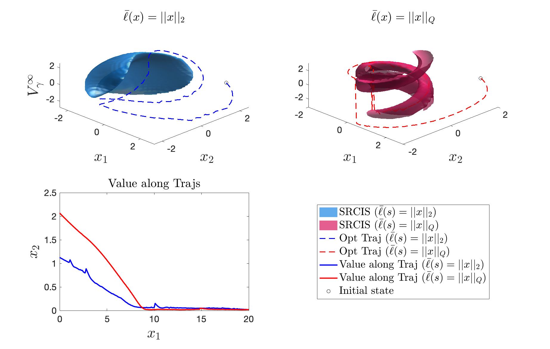
5.2 3D Dubins Car

Consider the 3D Dubins car example:

\displaystyle\dot{x}=v\cos(\theta)+d_{x},\hskip 10.00002pt\dot{y}=v\sin(\theta)+d_{y},\hskip 10.00002pt\dot{\theta}=u,

where $v=1$ and $u\in[-\pi/2,\pi/2]$ is the control and $d_{x},d_{y}\in[-0.1,0.1]$ is the disturbance. This system has no equilibrium point. The SRCISs With different $\bar{\ell}(x)$ are shown in Fig. 3, and the trajectory converges to the SRCIS exponentially.

5.3 10D Quadrotor

Consider the 10D quadrotor system:

		$\displaystyle\dot{x}=v_{x}+d_{x},\hskip 5.69054pt\dot{v_{x}}=g\tan{\theta_{x}},\hskip 5.69054pt\dot{\theta_{x}}=-d_{1}\theta_{x}+\omega_{x},$
		$\displaystyle\dot{\omega_{x}}=-d_{0}\theta_{x}+n_{0}u_{x},\hskip 5.69054pt\dot{y}=v_{y}+d_{y},\hskip 5.69054pt\dot{v_{y}}=g\tan{\theta_{y}},$
		$\displaystyle\dot{\theta_{y}}=-d_{1}\theta_{y}+\omega_{y},\hskip 5.69054pt\dot{\omega_{y}}=-d_{0}\theta_{y}+n_{0}u_{y},$
		$\displaystyle\dot{z}=v_{z}+d_{z},\hskip 5.69054pt\dot{v_{z}}=u_{z},$		(29)

where $(x,y,z)$ denote the position, $(v_{x},v_{y},v_{z})$ denote the velocity, $(\theta_{x},\theta_{y})$ denote the pitch and roll, $(\omega_{x},\omega_{y})$ denote the pitch and roll rates, and $(u_{x},u_{y},u_{z})$ are the controls. The system parameters are set to be $d_{0}=10,d_{1}=8,n_{0}=10,k_{T}=0.91,g=9.81$ , $|u_{x}|,|u_{y}|\leq\pi/9$ , $u_{z}\in[-1,1]$ , $|d_{x}|,|d_{y}|\leq 0.1$ , $|d_{z}|\leq 0.5$ .

This 10D system can be decomposed into three subsystems: X-sys with stats $[x,v_{x},\theta_{x},\omega_{x}]$ , Y-sys with stats $[y,v_{y},\theta_{y},\omega_{y}]$ , and Z-sys with stats $[z,v_{z}]$ . It can be verified that all three subsystems have an equilibrium point at the origin. Further, there’s no shared control or states among subsystems. We use $\bar{\ell}(x)=||x||_{2}$ .

Table 1: Comparison of the computation time for the 10D quadrotor. X/Y dim has 17 grids for each state, and Z dim has 101 grids for each state.

System	Z dim	X/Y dim	Full Sys
w/o Warmstrat	405.2 s	3731.7 s	7868.6s
w. Warmstart	234.9 s	3564.6 s	7364.1s

A CLF is reconstructed using equation (28), and the QP controllers for each subsystem are synthesized using Theorem 9. The results are shown in Fig. 4, and the computation time is shown in Tab. 1. A comparison of the R-CLVF with and without warmstart is shown in Fig. 5, showing that the warmstart provides the exact result.

6 Conclusions

In this paper, we extend our preliminary work on constructing CLVFs using HJ reachability analysis to the system with bounded disturbances. We provided more detailed discussions on several important claims and theorems compared to the previous version. Also, warmstarting and SCSD are proposed to solve the “curse of dimensionality,” and the effectiveness of both techniques is validated with numerical examples.

Future directions include finding conditions on when the SCSD provides R-CLVF and incorporating learning-based methods to tune the exponential rate $\gamma$ for online execution in robotics applications.

References

[1] E. D. Sontag, “A ‘universal’ construction of Artstein’s theorem on nonlinear stabilization,” Systems & control letters, 1989.
[2] R. A. Freeman and J. A. Primbs, “Control lyapunov functions: New ideas from an old source,” in Conf. on Decision and Control, 1996.
[3] K. K. Hassan et al., “Nonlinear systems,” Departement of Electrical and Computer Engineering, Michigan State University, 2002.
[4] A. D. Ames, S. Coogan, M. Egerstedt, G. Notomista, K. Sreenath, and P. Tabuada, “Control barrier functions: Theory and applications,” in European Control Conf., 2019.
[5] A. D. Ames, K. Galloway, K. Sreenath, and J. W. Grizzle, “Rapidly exponentially stabilizing control Lyapunov functions and hybrid zero dynamics,” Trans. on Automatic Control, 2014.
[6] A. Ames, X. Xu, J. W. Grizzle, and P. Tabuada, “Control barrier function based quadratic programs for safety critical systems,” Trans. on Automatic Control, 2017.
[7] Z. Artstein, “Stabilization with relaxed controls,” Nonlinear Analysis: Theory, Methods & Applications, 1983.
[8] F. Camilli, L. Grüne, and F. Wirth, “Control Lyapunov functions and Zubov’s method,” SIAM Journal on Control and Optimization, 2008.
[9] P. Giesl and S. Hafstein, “Review on computational methods for lyapunov functions,” Discrete & Continuous Dynamical Systems, 2015.
[10] P. Giesl, “Construction of a local and global lyapunov function for discrete dynamical systems using radial basis functions,” Journal of Approximation Theory, 2008.
[11] X. Xu, P. Tabuada, J. W. Grizzle, and A. D. Ames, “Robustness of control barrier functions for safety critical control,” Int. Federation of Automatic Control, 2015.
[12] S. Bansal, M. Chen, S. Herbert, and C. J. Tomlin, “Hamilton-Jacobi reachability: A brief overview and recent advances,” in Conf. on Decision and Control, 2017.
[13] L. C. Evans and P. E. Souganidis, “Differential games and representation formulas for solutions of Hamilton-Jacobi-Isaacs equations,” Indiana University Mathematics Journal, 1984.
[14] M. Bardi and I. Capuzzo-Dolcetta, Optimal control and viscosity solutions of Hamilton-Jacobi-Bellman equations. Springer, 2008.
[15] M. G. Crandall and P.-L. Lions, “Viscosity solutions of hamilton-jacobi equations,” Trans. of the American mathematical society, 1983.
[16] M. G. Crandall, L. C. Evans, and P.-L. Lions, “Some properties of viscosity solutions of hamilton-jacobi equations,” Trans. of the American Mathematical Society, 1984.
[17] H. Frankowska, “Hamilton-jacobi equations: viscosity solutions and generalized gradients,” Journal of mathematical analysis and applications, 1989.
[18] M. Chen, S. L. Herbert, M. S. Vashishtha, S. Bansal, and C. J. Tomlin, “Decomposition of reachable sets and tubes for a class of nonlinear systems,” Trans. on Automatic Control, 2018.
[19] S. Bansal and C. J. Tomlin, “Deepreach: A deep learning approach to high-dimensional reachability,” in Int. Conf. on Robotics and Automation, 2021.
[20] S. Herbert, J. J. Choi, S. Sanjeev, M. Gibson, K. Sreenath, and C. J. Tomlin, “Scalable learning of safety guarantees for autonomous systems using Hamilton-Jacobi reachability,” in Int. Conf. on Robotics and Automation, 2021.
[21] C. He, Z. Gong, M. Chen, and S. Herbert, “Efficient and guaranteed hamilton–jacobi reachability via self-contained subsystem decomposition and admissible control sets,” IEEE Control Systems Letters, vol. 7, pp. 3824–3829, 2023.
[22] Z. Gong, M. Zhao, T. Bewley, and S. Herbert, “Constructing control lyapunov-value functions using hamilton-jacobi reachability analysis,” IEEE Control Systems Letters, vol. 7, pp. 925–930, 2022.
[23] S. Rakovic, E. Kerrigan, K. Kouramas, and D. Mayne, “Invariant approximations of the minimal robust positively invariant set,” IEEE Transactions on Automatic Control, vol. 50, no. 3, pp. 406–410, 2005.
[24] Y. Chen, H. Peng, J. Grizzle, and N. Ozay, “Data-driven computation of minimal robust control invariant set,” in 2018 IEEE Conference on Decision and Control (CDC). IEEE, 2018, pp. 4052–4058.
[25] P. P. Varaiya, “On the existence of solutions to a differential game,” SIAM Journal on Control, vol. 5, no. 1, pp. 153–162, 1967.
[26] J. F. Fisac, M. Chen, C. J. Tomlin, and S. S. Sastry, “Reach-avoid problems with time-varying dynamics, targets and constraints,” in Hybrid Systems: Computation and Control. ACM, 2015.
[27] I. J. Fialho and T. T. Georgiou, “Worst case analysis of nonlinear systems,” Trans. on Automatic Control, 1999.
[28] J. J. Choi, D. Lee, K. Sreenath, C. J. Tomlin, and S. L. Herbert, “Robust control barrier-value functions for safety-critical control,” Conf. on Decision and Control, 2021.

		$\displaystyle\|\ell\big{(}\xi(s;t,x,u(\cdot),d(\cdot))\big{)}-\ell\big{(}\xi(s;t,y,u(\cdot),d(\cdot))\big{)}\|$
	$\displaystyle=$	$\displaystyle\big{\|}\|\|\xi(s;t,x,u(\cdot),d(\cdot))\|\|-\|\|\xi(s;t,y,u(\cdot),d(\cdot))\|\|\big{\|}$
	$\displaystyle\leq$	$\displaystyle\big{\|}\|\|\xi(s;t,x,u(\cdot),d(\cdot))-\xi(s;t,y,u(\cdot),d(\cdot))\|\|\big{\|}$
	$\displaystyle\leq$	$\displaystyle\big{\|}c\|\|x-y\|\|\big{\|}=c\|\|x-y\|\|.$

		$\displaystyle\|\|J_{\gamma}(t,x,u,d)-J_{\gamma}(t,y,u,d)\|\|$
	$\displaystyle=$	$\displaystyle\|\|\max_{s\in[t,0]}e^{\gamma(s-t)}\ell\big{(}\xi(s;t,x,u(\cdot),d(\cdot))\big{)}-$
		$\displaystyle\hskip 30.00005pt\max_{s\in[t,0]}e^{\gamma(s-t)}\ell\big{(}\xi(s;t,y,u(\cdot),d(\cdot))\big{)}\|\|$
	$\displaystyle\leq$	$\displaystyle\max_{s\in[t,0]}\|\|e^{\gamma(s-t)}\ell\big{(}\xi(s;t,x,u(\cdot),d(\cdot))\big{)}-$
		$\displaystyle\hskip 30.00005pte^{\gamma(s-t)}\ell\big{(}\xi(s;t,y,u(\cdot),d(\cdot))\big{)}\|\|$
	$\displaystyle\leq$	$\displaystyle\max_{s\in[t,0]}e^{\gamma(s-t)}c\|\|x-y\|\|=e^{-\gamma t}c\|\|x-y\|\|.$

		$\displaystyle e^{\gamma(s-t)}\bigl{(}\ell(\xi(s;t,x,u^{}(\cdot),\lambda[u^{}]))\bigl{)}$
	$\displaystyle\leq$	$\displaystyle e^{\gamma(s-t)}ke^{-\gamma(s-t)}\min_{a\in\partial\mathcal{I}_{m}}\|\|x-a\|\|$
	$\displaystyle=$	$\displaystyle k\min_{a\in\partial\mathcal{I}_{m}}\|\|x-a\|\|,$

		$\displaystyle\|\|\xi(s;t,x,u^{}(\cdot),\lambda[u^{}])\|\|$
	$\displaystyle=$	$\displaystyle V_{\gamma}\big{(}\xi(s;t,x,u^{}(\cdot),\lambda[u^{}]),0\big{)}+V^{\infty}_{m}$
	$\displaystyle\leq$	$\displaystyle V_{\gamma}^{\infty}\big{(}\xi(s;t,x,u^{}(\cdot),\lambda[u^{}])\big{)}+V^{\infty}_{m}.$

		$\displaystyle\min_{a\in\partial\mathcal{I}_{m}}\|\|\xi(s;t,x,u^{}(\cdot),\lambda[u^{}])-a\|\|$
	$\displaystyle\leq$	$\displaystyle\|\|\xi(s;t,x,u^{}(\cdot),\lambda[u^{}])\|\|+\min_{a\in\partial\mathcal{I}_{m}}\|\|a\|\|$
	$\displaystyle\leq$	$\displaystyle\|\|\xi(s;t,x,u^{}(\cdot),\lambda[u^{}])\|\|+V^{\infty}_{m}$
	$\displaystyle\leq$	$\displaystyle V_{\gamma}^{\infty}\big{(}\xi(s;t,x,u^{}(\cdot),\lambda[u^{}])\big{)}+2V^{\infty}_{m}$